Semileptonic Decays of $B$ Meson Transition Into $D$-wave Charmed Meson Doublets

Abstract

We use QCD sum rules to estimate the leading-order universal form factors describing the semileptonic $B$ decay into orbital excited $D$-wave charmed doublets, including the ($1^{-}$, $2^{-}$) states ($D_{1}^{*}$, $D^{\prime}_{2}$) and the ($2^{-}$, $3^{-}$) states ($D_{2}$, $D_{3}^{*}$). The decay rates we predict are $\Gamma_{B\rightarrow D^{*}_{1}\ell\overline{\nu}}=\Gamma_{B\rightarrow D^{\prime}_{2}\ell\overline{\nu}}=2.4\times 10^{-18}\mbox{GeV}$, $\Gamma_{B\rightarrow D_{2}\ell\overline{\nu}}=6.2\times 10^{-17}\mbox{GeV}$, and $\Gamma_{B\rightarrow D_{3}^{*}\ell\overline{\nu}}=8.6\times 10^{-17}\mbox{GeV}$. The branching ratios are $\mathcal{B}(B\rightarrow D^{*}_{1}\ell\overline{\nu})=\mathcal{B}(B\rightarrow D^{\prime}_{2}\ell\overline{\nu})=6.0\times 10^{-6}$, $\mathcal{B}(B\rightarrow D_{2}\ell\overline{\nu})=1.5\times 10^{-4}$, and $\mathcal{B}(B\rightarrow D_{3}^{*}\ell\overline{\nu})=2.1\times 10^{-4}$, respectively.

I Introduction

Higher excitations than $D^{(*)}$ play an important role in the understanding of semileptonic $B$ decays. Knowledge of these processes is important to reduce the uncertainties of the measurements on other semileptonic $B$ decays, and thus the determination of the Cabibbo-Kobayashi-Maskawa matrix elements, such as $|V_{cb}|$. Theoretically, the semileptonic decay processes are described by some form factors. The challenge for theory is the calculation of these decay form factors. Fortunately, the heavy quark effective theory (HQET) Wis , with an expansion in terms of $1/m_{Q}$ for hadrons containing a single heavy quark, provides a systematic method for investigating such processes. In HQET the approximate symmetries allow one to organize the spectrum of heavy mesons according to parity $P$ and total angular momentum $s_{l}$ of the light degree of freedom. Coupling the spin of the light degrees of freedom $s_{l}$ with the spin of a heavy quark $s_{Q}=1/2$ yields a doublet of meson states with a total spin $s=s_{l}\pm 1/2$. For charmed mesons, the lowest lying states $(0^{-},1^{-})$ doublet ($D$, $D^{*}$) are $S$-wave states with the spin of light degrees $s_{l}=1/2$. The $P$-wave excitation corresponds to two series of states, one is the $s_{l}=1/2$ series, the $(0^{+},1^{+})$ doublet ($D_{0}^{*}$, $D^{\prime}_{1}$); the other is the $s_{l}=3/2$ series, the $(1^{+},2^{+})$ doublet ($D_{1}$, $D^{*}_{2}$). For $D$-wave states, those are $(1^{-},2^{-})$ and $(2^{-},3^{-})$ doublets (($D_{1}^{*}$, $D^{\prime}_{2}$) and ($D_{2}$, $D^{*}_{3}$)), corresponding to the spin of light degrees of freedom $s_{l}=3/2$ and $s_{l}=5/2$. The early study of the heavy-light mesons can be found in Ref. God . The $S$-wave and $P$-wave charmed states have been observed so far. The properties of these states have been extensively studied using different approaches during the past few years, including masses Ebe ; Dai , decay constants Neu ; Cap ; Cve , and decay widths Dai3 ; Dai2 ; Eic ; Xia . For the $D$-wave charmed mesons, their properties were investigated with the potential model Eic and QCD sum rules Wei .

Semileptonic $B$ decay into an excited heavy meson has been observed in experiments Cle ; Ale . Recently, BABAR has measured semileptonic $B$ decays into orbitally excited charmed mesons $D_{1}(2420)$ and $D^{*}_{2}(2460)$ Aub1 . They also reported two new $D_{s}$ states $D_{sJ}(2860)$ and $D_{sJ}(2690)$ in the $DK$ channel, which may fit in the $D$-wave charm-strange doublets Aub . A similar state $D_{sJ}(2715)$ has also been observed by Belle Bel . It is expected that the nonstrange $D$-wave charmed mesons will be found, and the measurements of the semileptonic $B$ decays into these states become available in the near future. To this end we study the predictions of HQET for semileptonic $B$ decays to $D$-wave charmed mesons.

The semileptonic decay rate of a B meson transition into an charmed meson is determined by the corresponding matrix elements of the weak axial-vector and vector currents. In the heavy quark limit these elements are described, respectively, by one universal Isgur-Wise function at the leading order of heavy quark expansion Wis1 . The universal Isgur-Wise function is a nonperturbtive parameter. It must be calculated in some nonperturbative approaches. The main theoretical approaches are QCD sum rules Shi , constituent quark models, and lattice QCD. The investigations of semileptonic $B$ decays into charmed mesons can be found in Refs. Neu ; Hua1 ; Ebe1 ; Dea ; Wis1 with different methods. In this work, we estimate the leading-order Isgur-Wise functions describing the decays $B\rightarrow(D_{1}^{*},D^{\prime}_{2})\ell\overline{\nu}$ and $B\rightarrow(D_{2},D_{3}^{*})\ell\overline{\nu}$ and give a prediction for the widths of the decays.

The remainder of this paper is organized as follows. In Sec. II we present the formulas of weak current matrix elements and decay rates. In Sec. III we give the relevant sum rules for two-point correlators, and then deduce the three-point sum rules for the Isgur-Wise functions. Section IV is devoted to numerical results and discussions.

II Analytic formulations for semileptonic decay amplitudes $B\rightarrow(D_{1}^{*},D^{\prime}_{2})\ell\overline{\nu}$ and $B\rightarrow(D_{2},D_{3}^{*})\ell\overline{\nu}$

The heavy-light meson doublets can be expressed conveniently by effective operators Fal . For the ground doublet, the operator is

$$H_{a}=\frac{1+\hbox to0.0pt{/\hss}v}{2}[D^{*}_{\mu}\gamma^{\mu}-D\gamma_{5}].$$ (1)

The effective operators describing the meson doublets $D(1^{-},2^{-})$ and $D(2^{-},3^{-})$ are given by

$$X^{\mu}=\frac{1+\hbox to0.0pt{/\hss}v}{2}[D^{\prime\mu\nu}_{2}\gamma_{5}\gamma_{\nu}-D^{*}_{1\nu}\sqrt{\frac{3}{2}}(g^{\mu\nu}-\frac{1}{3}\gamma^{\nu}(\gamma^{\mu}+v^{\mu}))],$$ (2)

and

$$H^{\mu\nu}=\frac{1+\hbox to0.0pt{/\hss}v}{2}[D^{*\mu\nu\sigma}_{3}\gamma_{\sigma}-\sqrt{\frac{3}{5}}\gamma_{5}D^{\alpha\beta}_{2}(g^{\mu}_{\alpha}g^{\nu}_{\beta}-\frac{\gamma_{\alpha}}{5}g^{\nu}_{\beta}(\gamma^{\mu}-v^{\mu})-\frac{\gamma_{\beta}}{5}g^{\mu}_{\alpha}(\gamma^{\nu}-v^{\nu}))].$$ (3)

In these operators, $D^{*}_{\mu}$, $D$, $D^{\prime\mu\nu}_{2}$, $D^{*}_{1\nu}$, $D^{*\mu\nu\sigma}_{3}$, and $D^{\alpha\beta}_{2}$ separately represent annihilation operators of the $Q\overline{q}$ mesons with appropriate quantum numbers and $\hbox to0.0pt{/\hss}v=v\cdot\gamma$, $v$ is the heavy meson velocity. The theoretical description of semileptonic decays involves the matrix elements of vector and axial-vector currents ($V^{\mu}=\overline{c}\gamma^{\mu}b$ and $A^{\mu}=\overline{c}\gamma^{\mu}\gamma_{5}b$) between $B$ mesons and excited $D$ mesons. For the processes $B\rightarrow(D^{*}_{1},D^{\prime}_{2})\ell\overline{\nu}$ and $B\rightarrow(D_{2},D_{3}^{*})\ell\overline{\nu}$, these matrix elements can be parametrized through applying the trace formalism as follows Fal :

$$\langle D^{*}_{1}(v^{{}^{\prime}},\varepsilon)|(V-A)^{\mu}|B(v)\rangle = \sqrt{\frac{3}{2}}\sqrt{m_{B}m_{D^{*}_{1}}}\tau_{1}(y)[\varepsilon^{*}\cdot v(v^{\mu}-\frac{y+2}{3}v^{\prime\mu})$$ (4)

$$- i\frac{1-y}{3}\epsilon^{\mu\alpha\beta\sigma}\varepsilon^{*}_{\alpha}v^{\prime}_{\beta}v_{\sigma}],$$

$$\langle D^{\prime}_{2}(v^{{}^{\prime}},\varepsilon)|(V-A)^{\mu}|B(v)\rangle=\sqrt{m_{B}m_{D^{\prime}_{2}}}\tau_{1}(y)\varepsilon^{*}_{\rho\nu}v^{\rho}[g^{\mu\nu}(y-1)-v^{\nu}v^{{}^{\prime}\mu}+i\epsilon^{\alpha\beta\nu\mu}v^{{}^{\prime}}_{\alpha}v_{\beta}],$$ (5)

and

$$\langle D_{2}(v^{{}^{\prime}},\varepsilon)|(V-A)^{\mu}|B(v)\rangle = \sqrt{\frac{5}{3}}\sqrt{m_{B}m_{D_{2}}}\tau_{2}(y)\varepsilon^{*}_{\alpha\beta}v^{\alpha}[\frac{2(1-y^{2})}{5}g^{\mu\beta}-v^{\beta}v^{\mu}+\frac{2y-3}{5}v^{\beta}v^{{}^{\prime}\mu}$$ (6)

$$+ i\frac{2(1+y)}{5}\epsilon^{\mu\lambda\beta\rho}v_{\lambda}v^{{}^{\prime}}_{\rho}],$$

$$\langle D_{3}^{*}(v^{{}^{\prime}},\varepsilon)|(V-A)^{\mu}|B(v)\rangle=\sqrt{m_{B}m_{D_{3}^{*}}}\tau_{2}(y)\varepsilon^{*}_{\alpha\beta\lambda}v^{\alpha}v^{\beta}[g^{\mu\lambda}(1+y)-v^{\lambda}v^{{}^{\prime}\mu}+i\epsilon^{\mu\lambda\rho\tau}v_{\rho}v^{{}^{\prime}}_{\tau}],$$ (7)

where $(V-A)^{\mu}=\overline{c}\gamma^{\mu}(1-\gamma_{5})b$ is the weak current, $y=v\cdot v^{{}^{\prime}}$ and $\tau_{1}(y)$, $\tau_{2}(y)$ are the universal form factors, and $\varepsilon^{*}_{\alpha}$, $\varepsilon^{*}_{\alpha\beta}$, $\varepsilon^{*}_{\alpha\beta\lambda}$ are the polarization tensors of these mesons. The differential decay rates are calculated by making use of the formulas (4) to (7) given above:

$$\frac{d\Gamma}{dy}(B\rightarrow D^{*}_{1}\ell\overline{\nu})=\frac{G^{2}_{F}V^{2}_{cb}m^{2}_{B}m^{3}_{D^{*}_{1}}}{72\pi^{3}}(\tau_{1}(y))^{2}(y-1)^{\frac{5}{2}}(y+1)^{\frac{3}{2}}[(1+r_{1}^{2})(2y+1)-2r_{1}(y^{2}+y+1)],$$ (8)

$$\frac{d\Gamma}{dy}(B\rightarrow D^{\prime}_{2}\ell\overline{\nu})=\frac{G^{2}_{F}V^{2}_{cb}m^{2}_{B}m^{3}_{D^{\prime}_{2}}}{72\pi^{3}}(\tau_{1}(y))^{2}(y-1)^{\frac{5}{2}}(y+1)^{\frac{3}{2}}[(1+r_{2}^{2})(4y-1)-2r_{2}(3y^{2}-y+1)],$$ (9)

$$\frac{d\Gamma}{dy}(B\rightarrow D_{2}\ell\overline{\nu})=\frac{G^{2}_{F}V^{2}_{cb}m^{2}_{B}m^{3}_{D_{2}}}{360\pi^{3}}(\tau_{2}(y))^{2}(y-1)^{\frac{5}{2}}(y+1)^{\frac{7}{2}}[(1+r_{3}^{2})(7y-3)-2r_{3}(4y^{2}-3y+3)],$$ (10)

$$\frac{d\Gamma}{dy}(B\rightarrow D_{3}^{*}\ell\overline{\nu})=\frac{G^{2}_{F}V^{2}_{cb}m^{2}_{B}m^{3}_{D_{3}^{*}}}{360\pi^{3}}(\tau_{2}(y))^{2}(y-1)^{\frac{5}{2}}(y+1)^{\frac{7}{2}}[(1+r_{4}^{2})(11y+3)-2r_{4}(8y^{2}+3y+3)],$$ (11)

with $r_{i}=\frac{m_{D_{i}}}{m_{B}}$ ($D_{i}=D^{*}_{1},D^{\prime}_{2},D_{2},D^{*}_{3}$ for $i=1,2,3,4$ ). In the equations above, we have presented the decay rates of B semileptonic decay processes $B\rightarrow(D^{*}_{1},D^{\prime}_{2})\ell\overline{\nu}$ and $B\rightarrow(D_{2},D^{*}_{3})\ell\overline{\nu}$ in terms of the universal form factors $\tau_{1}(y)$ and $\tau_{2}(y)$, respectively. The only unknown factors in these equations are $\tau_{1}(y)$ and $\tau_{2}(y)$, which need to be determined by nonperturbative methods.

III Sum rules for Isgur-Wise functions

In the calculation of Isgur-Wise functions in HQET by means of QCD sum rule, the interpolating currents are potentially important. In Ref. Dai , two series of interpolating currents with nice propertties were proposed:

$$J^{{\dagger}\alpha_{1}\ldots\alpha_{j}}_{j,P,i}=\overline{h}_{v}(x)\Gamma^{\{\alpha_{1}\ldots\alpha_{j}\}}_{j,P,i}(D_{x_{t}})q(x)$$ (12)

or

$$J^{{}^{\prime}{\dagger}\alpha_{1}\ldots\alpha_{j}}_{j,P,i}=\overline{h}_{v}(x)\Gamma^{\{\alpha_{1}\ldots\alpha_{j}\}}_{j,P,i}(D_{x_{t}})(-i)\hbox to0.0pt{/\hss}D_{x_{t}}q(x)$$ (13)

where $i=1,2$ corresponding to two series of doublets of the spin-parity $[j^{(-1)^{j+1}},(j+1)^{(-1)^{j+1}}]$ and $[j^{(-1)^{j}},(j+1)^{(-1)^{j}}]$, respectively. $D_{t\mu}=D_{\mu}-v_{\mu}(v\cdot D)$ is the transverse component of the covariant derivative with respect to the velocity of the meson and

$$\Gamma^{\{\alpha_{1}\ldots\alpha_{j}\}}(D_{x_{t}})=\text{symmetrize}\{\Gamma^{\alpha_{1}\ldots\alpha_{j}}(D_{x_{t}})-\frac{1}{3}g^{\alpha_{1}\alpha_{2}}_{t}g^{t}_{\alpha^{{}^{\prime}}_{1}\alpha^{{}^{\prime}}_{2}}\Gamma^{\alpha^{{}^{\prime}}_{1}\alpha^{{}^{\prime}}_{2}\alpha_{3}\cdots\alpha_{j}}\}$$ (14)

with the transverse metric $g^{\alpha\beta}_{t}=g^{\alpha\beta}-v^{\alpha}v^{\beta}$. For the doublets of spin-parity $[j^{(-1)^{j+1}},(j+1)^{(-1)^{j+1}}]$ and $[j^{(-1)^{j}},(j+1)^{(-1)^{j}}]$, the expressions for $\Gamma^{\alpha_{1}\ldots\alpha_{j}}(D_{x_{t}})$ have been explicitly given in Dai as

$$\Gamma(D_{x_{t}})=\left\{\begin{tabular}[]{ll}$\sqrt{\frac{2j+1}{2j+2}}\gamma^{5}(-i)^{j}D^{\alpha_{2}}_{x_{t}}\cdots D^{\alpha_{j}}_{x_{t}}(D^{\alpha_{1}}_{x_{t}}-\frac{j}{2j+1}\gamma^{\alpha_{1}}_{t}\hbox to0.0pt{/\hss}D_{x_{t}})$,&for $j^{(-1)^{j+1}}$\\ $\frac{1}{\sqrt{2}}\gamma^{\alpha_{1}}_{t}(-i)^{j}D^{\alpha_{2}}_{x_{t}}\cdots D^{\alpha_{j}}_{x_{t}}$,&for $(j+1)^{(-1)^{j+1}}$\end{tabular}\right.$$

$$\Gamma(D_{x_{t}})=\left\{\begin{tabular}[]{ll}\ $\frac{1}{\sqrt{2}}\gamma^{5}(-i)^{j}\gamma^{\alpha_{1}}_{t}D^{\alpha_{2}}_{x_{t}}\cdots D^{\alpha_{j+1}}_{x_{t}}$,&for $(j+1)^{(-1)^{j}}$\\ $\sqrt{\frac{2j+1}{2j+2}}(-i)^{j}D^{\alpha_{2}}_{x_{t}}\cdots D^{\alpha_{j}}_{x_{t}}(D^{\alpha_{1}}_{x_{t}}-\frac{j}{2j+1}\gamma^{\alpha_{1}}_{t}\hbox to0.0pt{/\hss}D_{x_{t}})$,&for $j^{(-1)^{j}}$\end{tabular}\right.$$

where $\gamma_{t\mu}=\gamma_{\mu}-\hbox to0.0pt{/\hss}vv_{\mu}$ is the transverse component of $\gamma_{\mu}$ with respect to the heavy quark velocity.

For the $D$-wave meson doublets with $s_{l}=\frac{3}{2}^{-}$ and $s_{l}=\frac{5}{2}^{-}$, where $j=1$ and $j=2$, the currents are given by the following expressions:

$$J^{{\dagger}\alpha}_{1,-,3/2}=-i\sqrt{\frac{3}{4}}\overline{h}_{v}(D^{\alpha}_{t}-\frac{1}{3}\gamma^{\alpha}_{t}\hbox to0.0pt{/\hss}D_{t})q,$$ (15)

$$J^{{\dagger}\alpha\beta\lambda}_{2,-,3/2}=-i\frac{1}{\sqrt{2}}T^{\alpha\beta,\mu\nu}\overline{h}_{v}\gamma_{5}\gamma_{t\mu}D_{t\nu}q,$$ (16)

and

$$J^{{\dagger}\alpha\beta}_{2,-,5/2}=-\sqrt{\frac{5}{6}}T^{\alpha\beta,\mu\nu}\overline{h}_{v}\gamma_{5}(D_{t\mu}D_{t\nu}-\frac{2}{5}D_{t\mu}\gamma_{t\nu}\hbox to0.0pt{/\hss}D_{t})q,$$ (17)

$$J^{{\dagger}\alpha\beta\lambda}_{3,-,5/2}=-\frac{1}{\sqrt{2}}T^{\alpha\beta\lambda,\mu\nu\sigma}\overline{h}_{v}\gamma_{t\mu}D_{t\nu}D_{t\sigma}q,$$ (18)

which correspond to Eq. (12), and corresponding to Eq. (13) are

$$J^{{\dagger}\alpha}_{1,-,3/2}=-\sqrt{\frac{3}{4}}\overline{h}_{v}(D^{\alpha}_{t}-\frac{1}{3}\gamma^{\alpha}_{t}\hbox to0.0pt{/\hss}D_{t})\hbox to0.0pt{/\hss}D_{t}q,$$ (19)

$$J^{{\dagger}\alpha\beta\lambda}_{2,-,3/2}=-\frac{1}{\sqrt{2}}T^{\alpha\beta,\mu\nu}\overline{h}_{v}\gamma_{5}\gamma_{t\mu}D_{t\nu}\hbox to0.0pt{/\hss}D_{t}q,$$ (20)

and

$$J^{{\dagger}\alpha\beta}_{2,-,5/2}=-\sqrt{\frac{5}{6}}T^{\alpha\beta,\mu\nu}\overline{h}_{v}\gamma_{5}(D_{t\mu}D_{t\nu}-\frac{2}{5}D_{t\mu}\gamma_{t\nu}\hbox to0.0pt{/\hss}D_{t})(-i)\hbox to0.0pt{/\hss}D_{t}q,$$ (21)

$$J^{{\dagger}\alpha\beta\lambda}_{3,-,5/2}=-\frac{1}{\sqrt{2}}T^{\alpha\beta\lambda,\mu\nu\sigma}\overline{h}_{v}\gamma_{t\mu}D_{t\nu}D_{t\sigma}(-i)\hbox to0.0pt{/\hss}D_{t}q,$$ (22)

where $h_{v}$ is the generic velocity-dependent heavy quark effective field in HQET and $q$ denotes the light quark field. The tensors $T^{\alpha\beta,\mu\nu}$ and $T^{\alpha\beta\lambda,\mu\nu\sigma}$ are used to symmetrize indices and are given by Dai

$$T^{\alpha\beta,\mu\nu}=\frac{1}{2}(g^{\alpha\mu}_{t}g^{\beta\nu}_{t}+g^{\alpha\nu}_{t}g^{\beta\mu}_{t})-\frac{1}{3}g^{\alpha\beta}_{t}g^{\mu\nu}_{t},$$ (23)

$$T^{\alpha\beta\lambda,\mu\nu\sigma} = \frac{1}{6}(g^{\alpha\mu}_{t}g^{\beta\nu}_{t}g^{\lambda\sigma}_{t}+g^{\alpha\mu}_{t}g^{\beta\sigma}_{t}g^{\lambda\nu}_{t}+g^{\alpha\nu}_{t}g^{\beta\mu}_{t}g^{\lambda\sigma}_{t}+g^{\alpha\nu}_{t}g^{\beta\sigma}_{t}g^{\lambda\mu}_{t}+g^{\alpha\sigma}_{t}g^{\beta\nu}_{t}g^{\lambda\mu}_{t}+g^{\alpha\sigma}_{t}g^{\beta\mu}_{t}g^{\lambda\nu}_{t})$$ (24)

$$- \frac{1}{15}(g^{\alpha\beta}_{t}g^{\mu\nu}_{t}g^{\lambda\sigma}_{t}+g^{\alpha\beta}_{t}g^{\mu\sigma}_{t}g^{\lambda\nu}_{t}+g^{\alpha\beta}_{t}g^{\nu\sigma}_{t}g^{\lambda\mu}_{t}+g^{\alpha\lambda}_{t}g^{\mu\nu}_{t}g^{\beta\sigma}_{t}+g^{\alpha\lambda}_{t}g^{\mu\sigma}_{t}g^{\beta\nu}_{t}$$

$$+ g^{\alpha\lambda}_{t}g^{\nu\sigma}_{t}g^{\beta\mu}_{t}+g^{\beta\lambda}_{t}g^{\mu\nu}_{t}g^{\alpha\sigma}_{t}+g^{\beta\lambda}_{t}g^{\mu\sigma}_{t}g^{\alpha\nu}_{t}+g^{\beta\lambda}_{t}g^{\nu\sigma}_{t}g^{\alpha\mu}_{t}).$$

Usually the currents with derivatives of the lowest order (12) are used in the QCD sum rule approach. However, currents with derivatives of one order higher (13) are also used in some conditions because in the nonrelativistic quark model there is a corresponding relation between the orbital angular momenta and the orders of derivatives in the space wave functions. As for the orbital D-wave mesons, which corresponding to derivatives of order two, it is reasonable to use the currents (17), (18), (19) and (20).

These currents have nice properties, they have nonvanishing projection only to the corresponding states of the HQET in the $m_{Q}\rightarrow\infty$ limit, without mixing with states of the same quantum number but different $s_{l}$. Thus we can define one-particle-current couplings as follows:

$$J^{P}=1^{-}:\langle D^{*}_{1}(v,\varepsilon)|J^{\alpha}|0\rangle=f_{1}\sqrt{m_{D^{*}_{1}}}\varepsilon^{*\alpha},$$ (25)

$$J^{P}=2^{-}:\langle D^{\prime}_{2}(v,\varepsilon)|J^{\alpha\beta}|0\rangle=f^{\prime}_{2}\sqrt{m_{D^{\prime}_{2}}}\varepsilon^{*\alpha\beta},$$ (26)

$$J^{P}=2^{-}:\langle D_{2}(v,\varepsilon)|J^{\alpha\beta}|0\rangle=f_{2}\sqrt{m_{D_{2}}}\varepsilon^{*\alpha\beta},$$ (27)

$$J^{P}=3^{-}:\langle D^{*}_{3}(v,\varepsilon)|J^{\alpha\beta\lambda}|0\rangle=f_{3}\sqrt{m_{D^{*}_{3}}}\varepsilon^{*\alpha\beta\lambda}.$$ (28)

The couplings $f_{i}$ are low-energy parameters which are determined by the dynamics of the light degree of freedom. Since the pairs ($f_{1}$, $f^{\prime}_{2}$) and ($f_{2}$, $f_{3}$) are related by the spin symmetry, we will consider $f_{1}$ and $f_{2}$ hereafter. The decay constants $f_{i}$ can be estimated from two-point sum rules, therefore we list the sum rules after the Borel transformation. For the ground-state heavy mesons, the sum rule for the correlator of two heavy-light currents is well known. It is Hua1

$$f^{2}_{-,\frac{1}{2}}e^{-2\bar{\Lambda}_{-,\frac{1}{2}}/T}=\frac{3}{16\pi^{2}}\int_{0}^{\omega_{c0}}\omega^{2}e^{-\omega/T}d\omega-\frac{1}{2}\langle\bar{q}q\rangle(1-\frac{m^{2}_{0}}{4T^{2}}).$$ (29)

For the $s_{l}^{P}=\frac{3}{2}^{-}$ doublet, when the currents (19) and (20) are used, the corresponding sum rule is :

$$f^{2}_{-,\frac{3}{2}}e^{-2\bar{\Lambda}_{-,\frac{3}{2}}/T}=\frac{1}{2^{8}\pi^{2}}\int_{0}^{\omega_{c1}}\omega^{6}e^{-\omega/T}d\omega-\frac{5}{3\times 2^{8}}\int_{0}^{\omega_{c1}}\omega^{2}e^{-\omega/T}d\omega\langle\frac{\alpha_{s}}{\pi}GG\rangle.$$ (30)

For the $s_{l}^{P}=\frac{5}{2}^{-}$ doublet, when the currents (17) and (18) are used, the corresponding sum rule is :

$$f^{2}_{-,\frac{5}{2}}e^{-2\bar{\Lambda}_{-,5/2}/T}=\frac{1}{5\times 2^{7}\pi^{2}}\int_{0}^{\omega_{c2}}\omega^{6}e^{-\omega/T}d\omega-\frac{5}{3\times 2^{6}}\int_{0}^{\omega_{c2}}\omega^{2}e^{-\omega/T}d\omega\langle\frac{\alpha_{s}}{\pi}GG\rangle.$$ (31)

As we have just mentioned, for the amplitudes of the semileptonic decays into excited states in the infinite mass limit, the only unknown quantities in (8), (9), (10) and (11) are the universal functions $\tau_{1}(y)$ and $\tau_{2}(y)$. In Ref. Col the form factors $\tau_{1}(y)$ and $\tau_{2}(y)$ were estimated through QCD sum rule by using currents with derivatives of lower order, (15) to (18). Considering that the corresponding relation between the orbital angular momentum and the order of the derivative mentioned above, we use the currents (19) and (20) instead of (15) and (16) for the ($D_{1}^{*}$, $D^{\prime}_{2}$) doublet. As for the ($D_{2}$, $D^{*}_{3}$) doublet, we also use the currents (17) and (18).

In order to calculate this two form factors by QCD sum rules, we study the analytic properties of three-point correlators:

$$i^{2}\int d^{4}xd^{4}ze^{i(k^{{}^{\prime}}\cdot x-k\cdot z)}\langle 0|T[J^{\alpha}_{1,-}(x)J^{\mu(v,v^{{}^{\prime}})}_{V,A}(0)J^{{\dagger}}_{0,-}(z)|0\rangle=\Gamma(\omega,\omega^{{}^{\prime}},y)\mathcal{L}^{\mu\alpha}_{V,A},$$ (32)

$$i^{2}\int d^{4}xd^{4}ze^{i(k^{{}^{\prime}}\cdot x-k\cdot z)}\langle 0|T[J^{\alpha\beta}_{2,-}(x)J^{\mu(v,v^{{}^{\prime}})}_{V,A}(0)J^{{\dagger}}_{0,-}(z)|0\rangle=\Gamma^{\prime}(\omega,\omega^{{}^{\prime}},y)\mathcal{L}^{\mu\alpha\beta}_{V,A},$$ (33)

where $J^{\mu(v,v^{{}^{\prime}})}_{V}=h(v^{{}^{\prime}})\gamma^{\mu}h(v)$ and $J^{\mu(v,v^{{}^{\prime}})}_{A}=h(v^{{}^{\prime}})\gamma^{\mu}\gamma_{5}h(v)$. The variables $k$($=P-m_{b}v$) and $k^{{}^{\prime}}$($=P^{\prime}-m_{c}v^{\prime}$) denote residual “off-shell” momenta of the initial and final meson states, respectively. For heavy quarks in bound states they are typically of order $\Lambda_{QCD}$ and remain finite in the heavy quark limit. $\Gamma(\omega,\omega^{{}^{\prime}},y)$ and $\Gamma^{\prime}(\omega,\omega^{{}^{\prime}},y)$ are analytic functions in the “off-shell” energies $\omega=2v\cdot k$ and $\omega^{\prime}=2v^{\prime}\cdot k^{\prime}$ with discontinuities for positive values of these variables. They also depend on the velocity transfer $y=v\cdot v^{\prime}$, which is fixed in a physical region. $\mathcal{L}_{V,A}$ are Lorentz structures.

Following the standard QCD sum rule procedure, the calculations of $\Gamma(\omega,\omega^{{}^{\prime}},y)$ and $\Gamma^{\prime}(\omega,\omega^{{}^{\prime}},y)$ are straightforward. First, we saturate Eqs.(32) and (33) with physical intermediate states in HQET and find that the hadronic representations of the correlators as follows:

$$\Gamma_{hadron}(\omega,\omega^{{}^{\prime}},y)=\frac{f_{-,\frac{1}{2}}f_{-,j_{l}}\tau_{i}(y)}{(2\bar{\Lambda}_{-,\frac{1}{2}}-\omega-i\varepsilon)(2\bar{\Lambda}_{-,j_{l}}-\omega^{{}^{\prime}}-i\varepsilon)}+\text{higher resonances},$$ (34)

where $f_{-,j_{l}}$ are the decay constants defined in Eqs.(25) and (27), $\overline{\Lambda}_{-,j_{l}}=m_{-,j_{l}}-m_{Q}$. Second, the functions can be approximated by a perturbative calculation supplemented by nonperturbative power corrections proportional to the vacuum condensates which are treated as phenomenological parameters. The perturbative contribution can be represented by a double dispersion integral in $\nu$ and $\nu^{{}^{\prime}}$ plus possible subtraction terms. So the theoretical expression for the correlator has the form

$$\Gamma_{theo}(\omega,\omega^{{}^{\prime}},y)\simeq\int d\nu d\nu^{{}^{\prime}}\frac{\rho^{pert}(\nu,\nu^{{}^{\prime}},y)}{(\nu-\omega-i\varepsilon)(\nu^{{}^{\prime}}-\omega^{{}^{\prime}}-i\varepsilon)}+\text{subtractions}+\Gamma^{cond}(\omega,\omega^{{}^{\prime}},y).$$ (35)

The perturbative part of the spectral density can be calculated straightforward. Confining us to the leading order of perturbation, the perturbative spectral densities of the two sum rules for $\tau_{1}(y)$ and $\tau_{2}(y)$ are

$$\rho_{pert}(\nu,\nu^{{}^{\prime}},y)=\frac{3}{2^{8}\pi^{2}}\frac{1}{(y+1)^{\frac{3}{2}}(y-1)^{\frac{5}{2}}}\nu^{{}^{\prime}}[(3\nu^{2}-(1+2y)(2\nu\nu^{\prime}-\nu^{\prime 2})]$$

$$\times\Theta(\nu)\Theta(\nu^{{}^{\prime}})\Theta(2y\nu\nu^{{}^{\prime}}-\nu^{2}-\nu^{{}^{\prime}2}),$$ (36)

and

$$\rho_{pert}(\nu,\nu^{{}^{\prime}},y)=\frac{3}{2^{8}\pi^{2}}\frac{1}{(y+1)^{\frac{7}{2}}(y-1)^{\frac{5}{2}}}[(5\nu-12y\nu^{{}^{\prime}}+3\nu^{{}^{\prime}})\nu^{2}+(3\nu+\nu^{{}^{\prime}})(2y^{2}-2y+1)\nu^{{}^{\prime}2}]$$

$$\times\Theta(\nu)\Theta(\nu^{{}^{\prime}})\Theta(2y\nu\nu^{{}^{\prime}}-\nu^{2}-\nu^{{}^{\prime}2}).$$ (37)

Following the arguments in Refs. Neu ; Blo , the perturbative and the hadronic spectral densities cannot be locally dual to each other, the necessary way to restore duality is to integrate the spectral densities over the “off-diagonal” variable $\nu_{-}=\nu-\nu^{{}^{\prime}}$, keeping the “diagonal” variable $\nu_{+}=\frac{\nu+\nu^{{}^{\prime}}}{2}$ fixed. It is in $\nu_{+}$ that the quark-hadron duality is assumed for the integrated spectral densities. The integration region can be expressed in terms of the variables $\nu_{-}$ and $\nu_{+}$ and we choose the triangular region defined by the bounds: $0\leq\nu_{+}\leq\omega_{c}$, $-2\sqrt{\frac{y-1}{y+1}}\nu_{+}\leq\nu_{-}\leq 2\sqrt{\frac{y-1}{y+1}}\nu_{+}$. As discussed in Refs. Blo ; Neu , the upper limit $\omega_{c}$ for $\nu_{+}$ in the region $\frac{1}{2}[(y+1)-\sqrt{y^{2}-1}]\omega_{c0}\leqslant\omega_{c}\leqslant\frac{1}{2}(\omega_{c0}+\omega_{c2})$ is reasonable. A double Borel transformation in $\omega$ and $\omega^{{}^{\prime}}$ is performed on both sides of the sum rules, in which for simplicity we take the Borel parameters equal Neu ; Hua1 ; Col : $T_{1}=T_{2}=2T$. In the calculation, we have considered the operators of dimension $D\leq 5$ in OPE. After adding the nonperturbative parts, we obtain the sum rules for $\tau_{1}$ and $\tau_{2}$ as follows:

$$\tau_{1}(y)f_{-,1/2}f_{-,3/2}e^{-(\bar{\Lambda}_{-,1/2}+\bar{\Lambda}_{-,3/2})/T} = \frac{1}{2^{4}\pi^{2}}\frac{1}{(1+y)^{3}}\int^{\omega^{\prime}_{c}}_{0}d\nu_{+}e^{-\frac{\nu_{+}}{T}}\nu^{4}_{+}$$ (38)

$$- \frac{T}{3\times 2^{5}}\frac{2y+3}{(y+1)^{2}}\langle\frac{\alpha_{s}}{\pi}GG\rangle,$$

$$\tau_{2}(y)f_{-,1/2}f_{-,5/2}e^{-(\bar{\Lambda}_{-,1/2}+\bar{\Lambda}_{-,5/2})/T} = \frac{3}{8\pi^{2}}\frac{1}{(1+y)^{4}}\int^{\omega_{c}}_{0}d\nu_{+}e^{-\frac{\nu_{+}}{T}}\nu^{4}_{+}$$ (39)

$$- \frac{T}{3\times 2^{4}}\frac{1}{(y+1)^{3}}\langle\frac{\alpha_{s}}{\pi}GG\rangle.$$

We also derive the sum rule for $\tau_{2}$ by using the currents (21) and (22), which appears to be

$$\tau_{2}(y)f_{-,1/2}f_{-,5/2}e^{-(\bar{\Lambda}_{-,1/2}+\bar{\Lambda}_{-,5/2})/T} = \frac{21}{5\times 2^{4}\pi^{2}}\frac{1}{(1+y)^{4}}\int^{\omega_{c}}_{0}d\nu_{+}e^{-\frac{\nu_{+}}{T}}\nu^{5}_{+}$$ (40)

$$+ \frac{T^{2}}{3\times 2^{4}}\frac{4y-25}{(y+1)^{3}}\langle\frac{\alpha_{s}}{\pi}GG\rangle.$$

IV Numerical results and discussions

We now evaluate the sum rules numerically. For the QCD parameters entering the theoretical expressions, we take the standard values: $\langle\overline{q}q\rangle=-(0.24)^{3}\mbox{GeV}^{3}$, $\langle\alpha_{s}GG\rangle=0.04\mbox{GeV}^{4}$, and $m^{2}_{0}=0.8\mbox{GeV}^{2}$. In the numerical calculations, we take $2.83\mbox{GeV}$ God ; Eic for the mass of the $s_{l}=5/2$ doublet and $2.78\mbox{GeV}$ for the $s_{l}=3/2$ doublet. For mass of initial $B$ meson, we use $m_{B}=5.279\mbox{GeV}$ Pdg .

In order to obtain information of $\tau_{1}(y)$ and $\tau_{2}(y)$ with less systematic uncertainties in the calculation, we divide the three-point sum rules by the square roots of relevant two-point sum rules, as many authors did Neu ; Hua1 ; Col , to reduce the number of input parameters and improve stabilities. Then we obtain expressions for the $\tau_{1}(y)$ and $\tau_{2}(y)$ as functions of the Borel parameter $T$ and the continuum thresholds. Imposing usual criteria for the upper and lower bounds of the Borel parameter, we found they have a common sum rule “window”: $0.7\mbox{GeV}<T<1.5\mbox{GeV}$, which overlaps with those of two-point sum rules (29), (30) and (31) (see Fig. 1). Notice that the Borel parameter in the sum rules for three-point correlators is twice the Borel parameter in the sum rules for the two-point correlators. In the evaluation we have taken $2.0\mbox{GeV}<\omega_{c0}<2.4\mbox{GeV}$ Hua1 ; Neu , $2.8\mbox{GeV}<\omega_{c1}<3.2\mbox{GeV}$, and $3.2\mbox{GeV}<\omega_{c2}<3.6\mbox{GeV}$. The regions of these continuum thresholds are fixed by analyzing the corresponding two-point sum rules. According to the discussion in Sec. III, we can fix $\omega^{\prime}_{c}$ and $\omega_{c}$ in the regions $2.3\mbox{GeV}<\omega^{\prime}_{c}<2.6\mbox{GeV}$ and $2.5\mbox{GeV}<\omega_{c}<2.7\mbox{GeV}$. The results are showed in Fig. 2.

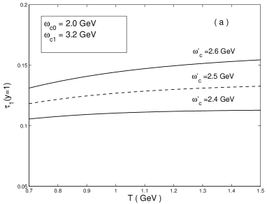
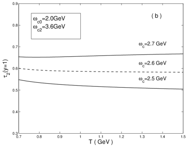
Figure 1: Dependence of $\tau_{1}(y)$ and $\tau_{2}(y)$ on Borel parameter $T$ at $y=1$.

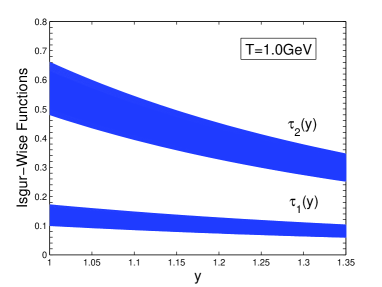
Figure 2: Prediction for the Isgur-Wise functions $\tau_{1}(y)$ and $\tau_{2}(y)$.

The resulting curves for $\tau_{1}(y)$ and $\tau_{2}(y)$ can be parametrized by the linear approximation

$$\tau_{1}(y)=\tau_{1}(1)[1-\rho^{2}_{\tau_{1}}(y-1)],\text{ }\tau_{1}(1)=0.14\pm 0.03,\text{ }\rho^{2}_{\tau_{1}}=0.13\pm 0.02;$$ (41)

$$\tau_{2}(y)=\tau_{2}(1)[1-\rho^{2}_{\tau_{2}}(y-1)],\text{ }\tau_{2}(1)=0.57\pm 0.09,\text{ }\rho^{2}_{\tau_{2}}=0.78\pm 0.13.$$ (42)

The errors mainly come from the uncertainty due to $\omega_{c}$’s and $T$. It is difficult to estimate these systematic errors which are brought in by the quark-hadron duality. The maximal values of $y$ are $y^{D^{*}_{1}}_{max}=y^{D^{\prime}_{2}}_{max}=(1+r_{1,2}^{2})/2r_{1,2}\approx 1.213$ and $y^{D_{2}}_{max}=y^{D^{*}_{3}}_{max}=(1+r_{3,4}^{2})/2r_{3,4}\approx 1.201$. By using the parameters $V_{cb}=0.04$, $G_{F}=1.166\times 10^{-5}\mbox{GeV}^{-2}$, we get the semileptonic decay rates of $B\rightarrow(D_{1}^{*},D^{\prime}_{2})\ell\overline{\nu}$ and $B\rightarrow(D_{2},D_{3}^{*})\ell\overline{\nu}$. Consider that $\tau_{B}=1.638\text{ps}$ Pdg , we get the branching ratios, respectively. All these results are listed in Table 1.

Table 1: Predictions for the decay widths and branching ratios

Decay mode		Decay width $\Gamma$ (GeV)		Branching ratio		Branching ratio of Ref.Col
$B\rightarrow D^{*}_{1}\ell\overline{\nu}$		$2.4\times 10^{-18}$		$6.0\times 10^{-6}$
$B\rightarrow D^{\prime}_{2}\ell\overline{\nu}$		$2.4\times 10^{-18}$		$6.0\times 10^{-6}$
$B\rightarrow D_{2}\ell\overline{\nu}$		$6.2\times 10^{-17}$		$1.5\times 10^{-4}$		$1\times 10^{-5}$
$B\rightarrow D^{*}_{3}\ell\overline{\nu}$		$8.6\times 10^{-17}$		$2.1\times 10^{-4}$		$1\times 10^{-5}$

Because of the large background from $B\rightarrow D^{(*)}\ell\overline{\nu}$ decays, there is no experimental data available so far. As we can see from Table 1, the rates of semileptonic $B$ decay into the $s^{P}_{l}=\frac{3}{2}^{-}$ doublet are tiny and our results are larger than those predicted by Ref. Col in the $B$ to $s^{P}_{l}=\frac{5}{2}^{-}$ charmed doublet channels. The difference comes because the way in which we choose the parameters is different from theirs. They chose the parameters according to other theoretical approaches. In contrast, we choose the parameters following the way of Ref. Neu . In addition, we also estimate the universal form factor $\tau_{2}(y)$ with the sum rule (40) and we get almost the same result as (42). When trying to estimate the $\tau_{1}(y)$ by using the currents (15) and (16), we find that after the quark-hadron duality are assumed the integral over the perturbative spectral density becomes zero. As for the $P$-wave and the $F$-wave mesons, similar results can be obtained after the calculations above have been carefully repeated.

The semileptonic and leptonic $B$ decay rate is about $10.9\%$ of the total $B$ decay rate, in which the $S$-wave charmed mesons $D$ and $D^{*}$ contribute about $8.65\%$ Pdg and the $P$-wave charmed mesons contribute about $0.9\%$ Hua1 . Our results then suggest that the $D$-wave charmed mesons contribute about $0.04\%$ of the total $B$ decay rate. Sum up the branching ratios of these semileptonic $B$ decay processes, the eight lightest charmed mesons contribute about $9.59\%$ of the $B$ decay rate. Therefore, semileptonic decays into higher excited states and nonresonant multibody channels should be about $1.31\%$ of the $B$ decay rate. Whatsoever, our result is just a leading-order estimate of the contribution of the $D$-wave charmed mesons channels to the semileptonic $B$ decay.

In summary, we estimate the leading-order universal form factors describing the $B$ meson of ground-state transition into orbital excited $D$-wave charmed resonances, the ($1^{-}$, $2^{-}$) states ($D_{1}^{*}$, $D^{\prime}_{2}$), which belong to the $s_{l}^{P}=\frac{3}{2}^{-}$ heavy quark doublet and the ($2^{-}$, $3^{-}$) states ($D_{2}$, $D^{*}_{3}$), which belong to the $s_{l}^{P}=\frac{5}{2}^{-}$ heavy quark doublet, by use of QCD sum rules within the framework of HQET. The semileptonic decay widths as well as the branching ratios we get are shown in Table 1. The predictions are larger than those predicted by Ref. Col . This needs future experiments for clarification. We also prove that when $s^{P}_{l}=\frac{5}{2}^{-}$ the interpolating currents (12) and (13) proposed in Ref. Dai are really equivalent. It is worth noting that in the estimate of the semileptonic $B$ decay form factors when the currents (12) with quantum numbers of light degree of freedom $s_{l}^{P}=\frac{1}{2}^{+},\frac{3}{2}^{-},\frac{5}{2}^{+}$ are used for the excited charmed mesons, we find the perturbative contributions vanish after the quark-hadron duality are assumed. In this case we should use the currents (13) which contain derivatives of one order higher.

References

• (1) M. Neubert, Phys. Rep. 245, 259 (1994) and references therein; Aneesh V. Mannohar and Mark B. Wise, Heavy Quark Physics, Cambridge University Press (2000).
• (2) S. Godfrey and R. Kokoski, Phys. Rev. D 43, 1679 (1991); S. Godfrey and N. Isgur, Phys. Rev. D 32, 189 (1985).
• (3) D. Ebert, V. O. Galkin and R. N. Faustov, Phys. Rev. D 57, 5663 (1998).
• (4) Y. B. Dai, C. S. Huang, M. Q. Huang, and C. Liu, Phys. Lett. B 390, 350 (1997); Y. B. Dai, C. S. Huang, and M. Q. Huang, Phys. Rev. D 55, 5719 (1997).
• (5) M. Neubert, Phys. Rev. D 45, 2451 (1992); 46, 3914 (1992).
• (6) S. Capstick and S. Godfrey, Phys. Rev. D 41, 2856 (1990).
• (7) G. Cvetič , C. S. Kim, Guo-Li Wang and Wuk Namgung, Phys. Lett. B 596, 84 (2004); Guo-Li Wang, Phys. Lett. B 633, 492 (2006).
• (8) Y. B. Dai, C. S. Huang, M. Q. Huang, H. Y. Jin, and C. Liu, Phys. Rev. D 58, 094032 (1998).
• (9) Y. B. Dai, C. S. Huang, and H. Y. Jin, Z. Phys. C 60, 527-534 (1993); Phys. Lett. B 331, 174 (1994); Y. B. Dai and H. Y. Jin, Phys. Rev. D 52, 236 (1995).
• (10) E. J. Eichten, C. T. Hill, and C. Quigg, Phys. Rev. Lett.71, 4116 (1993).
• (11) X. H. Zhong and Q. Zhao, Phys. Rev. D 78, 014029 (2007).
• (12) W. Wei, X. Liu, and S. L. Zhu, Phys. Rev. D 75, 014013 (2007).
• (13) A. Anastassov et al. (CLEO Collaboration), Phys. Rev. Lett. 80, 4127 (1998).
• (14) D. Buskulic et al. (ALEPH Collaboration), Phys. Lett. B 395, 373 (1997); Z. Phys. C 73, 601 (1997).
• (15) B. Aubert et al. (BARBAR Collaboration), hep-ex/0808.0333.
• (16) B. Aubert et al. (BARBAR Collaboration), Phys. Rev. Lett. 97, 222001 (2006).
• (17) K. Abe et al. (BELLE Collaboration), hep-ex/0608031.
• (18) A. K. Leibovich, Z. Ligeti, I. W. Stewart, and M. B. Wise, Phys. Rev. Lett.78, 3995 (1997); Phys. Rev. D 57, 308 (1998).
• (19) M. A. Shifman, A. I. Vainshtein, and V. I. Zakharov, Nucl. Phys. B 147, 385 (1979); 147, 448 (1979); V. A. Novikov, M. A. Shifman and A. I. Vainshtein, and V. I. Zakharov, Fortschr. Phys. 32, 585 (1984).
• (20) M. Q. Huang and Y. B. Dai, Phys. Rev. D 59, 034018 (1999); 64, 014034 (2001).
• (21) D. Ebert, R. N. Faustov and V. O. Galkin, Phys. Rev. D 61, 014016 (1999); 75, 074008 (2007).
• (22) A. Deandrea, N. Di Bartolomeo, R. Gatto, G. Nardulli and A. D. Polosa, Phys. Rev. D 58, 034004 (1998); V. MorΓ©nas, A. Le Yaouanc, L. Oliver, O. PΓ¨ne and J. C. Raynal, Phys. Rev. D 56, 5668 (1997).
• (23) A. F. Falk, Nul. Phys. B 378, 79 (1992); A. F. Falk and M. Luke, Phys. Lett. B 292, 119 (1992).
• (24) P. Colangelo, F. De Fazio and G. Nardulli, Phys. Lett. B 478, 408 (2000).
• (25) B. Blok and M. Shifman, Phys. Rev. D 47, 2949 (1993).
• (26) Particle Data Group, C. Amsler et al., Phys. Lett. B 667, 1 (2008).