Load optimization in a planar network

Abstract

We analyze the asymptotic properties of a Euclidean optimization problem on the plane. Specifically, we consider a network with three bins and $n$ objects spatially uniformly distributed, each object being allocated to a bin at a cost depending on its position. Two allocations are considered: the allocation minimizing the bin loads and the allocation allocating each object to its less costly bin. We analyze the asymptotic properties of these allocations as the number of objects grows to infinity. Using the symmetries of the problem, we derive a law of large numbers, a central limit theorem and a large deviation principle for both loads with explicit expressions. In particular, we prove that the two allocations satisfy the same law of large numbers, but they do not have the same asymptotic fluctuations and rate functions.

and

1 Introduction

In this paper we take an interest in a Euclidean optimization problem on the plane. For ease of notation, we shall identify the plane with the set of complex numbers $\mathbb{C}$. Set $\lambda=2(3\sqrt{3})^{-1/2}$, $i=\sqrt{-1}$ (the complex unit), $j={e}^{2i\pi/3}$ and consider the triangle $\mathbb{T}\subset\mathbb{C}$ with vertices $B_{2}=\lambda i$, $B_{1}=j^{2}B_{2}$ and $B_{3}=jB_{2}$. Note that $\mathbb{T}$ is an equilateral triangle with side length $\lambda\sqrt{3}$ and unit area. We label by $\{1,\ldots,n\}$ $n$ objects located in the interior of $\mathbb{T}$ and denote by $X_{k}$, $k=1,\ldots,n$, the location of the $k$th object; see Figure 1. We assume that $\{X_{k}\}_{k=1,\ldots,n}$ are independent random variables (r.v.’s) with uniform distribution on $\mathbb{T}$. Suppose that there are three bins located at each of the vertices of $\mathbb{T}$ and that each object has to be allocated to a bin. The cost of an allocation is described by a measurable function $c\dvtx\mathbb{T}\to[0,\infty)$ such that $\|c\|_{\infty}:=\sup_{x\in\mathbb{T}}c(x)<\infty$. More precisely, $c(x)=c_{1}(x)$ denotes the cost to allocate an object at $x\in\mathbb{T}$ to the bin in $B_{1}$; the cost to allocate an object at $x\in\mathbb{T}$ to the bin in $B_{2}$ is $c_{2}(x)=c(j^{2}x)$; the cost to allocate an object at $x\in\mathbb{T}$ to the bin in $B_{3}$ is $c_{3}(x)=c(jx)$. Let

$$\mathcal{A}_{n}=\bigl{\{}A=(a_{kl})_{1\leq k\leq n,1\leq l\leq 3}\dvtx a_{kl}\in\{0,1\},a_{k1}+a_{k2}+a_{k3}=1\bigr{\}}$$

be the set of allocation matrices: if $a_{kl}=1$ the $k$th object is affiliated to the bin in $B_{l}$. We consider the load relative to the allocation matrix $A=(a_{kl})_{1\leq k\leq n,1\leq l\leq 3}\in\mathcal{A}_{n}$:

$$\rho_{n}(A)=\max_{1\leq l\leq 3}\Biggl{(}\sum_{k=1}^{n}a_{kl}c_{l}(X_{k})\Biggr{)},$$

and the minimal load

$$\rho_{n}=\min_{A\in\mathcal{A}_{n}}\rho_{n}(A).$$

Throughout this paper we refer to $\rho_{n}$ as the optimal load. This simple instance of Euclidean optimization problem has potential applications in operations research and wireless communication networks. Consider three processors running in parallel and sharing a pool of tasks $\{1,\ldots,n\}$ located, respectively, at $\{X_{1},\ldots,X_{n}\}\subseteq\mathbb{T}$. Suppose that $c_{l}(x)$ is the time requested by the $l$th processor to process a job located at $x\in\mathbb{T}$. Then $\rho_{n}$ is the minimal time requested to process all jobs. For example, a natural choice for the cost function is $c(x)=2|x-B_{1}|$, that is, the time of a round-trip from $B_{1}$ to $x$ at unit speed. In a wireless communication scenario, the bins are base stations and the objects are users located at $\{X_{1},\ldots,X_{n}\}\subseteq\mathbb{T}$. For the base station located at $B_{l}$, the time needed to send one bit of information to a user located at $x\in\mathbb{T}$ is $c_{l}(x)$. In this context $\rho_{n}$ is the minimal time requested to send one bit of information to each user and $1/\rho_{n}$ is the maximal throughput that can be achieved. We have chosen a triangle $\mathbb{T}$ because it is the fundamental domain of the hexagonal grid, which is a good model for cellular wireless networks.

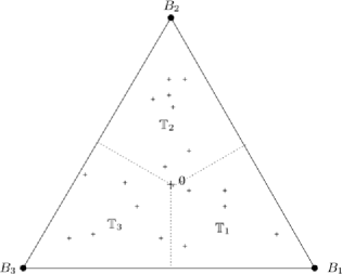
Figure 1: The triangle $\mathbb{T}$, the three bins and the $n$ objects.

For $1\leq l\leq 3$, we define the Voronoi cell associated to the bin at $B_{l}$ by

$$\mathbb{T}_{l}=\Bigl{\{}x\in\mathbb{T}\dvtx|x-B_{l}|={\min_{1\leq m\leq 3}}|x-B_{m}|\Bigr{\}}\bigm{\backslash}D_{l},$$

where $D_{1}=\{ijt\dvtx t<0\}$ and, for $l=2,3$, $D_{l}=\{ij^{l}t\dvtx t\leq 0\}$. Note that $\mathbb{T}_{1}\cup\mathbb{T}_{2}\cup\mathbb{T}_{3}=\mathbb{T}$ and $\mathbb{T}_{1}\cap\mathbb{T}_{2}=\mathbb{T}_{1}\cap\mathbb{T}_{3}=\mathbb{T}_{2}\cap\mathbb{T}_{3}=\varnothing$, that is, $\{\mathbb{T}_{1},\mathbb{T}_{2},\mathbb{T}_{3}\}$ is a partition of $\mathbb{T}$. Note also that $0\in\mathbb{T}_{1}$.

Throughout the paper, we denote by $|\cdot|$ the Euclidean norm on $\mathbb{C}$, by $\ell$ the Lebesgue measure on $\mathbb{C}$ and by $x\cdot z$ the usual scalar product on $\mathbb{C}$, that is, $x\cdot z=\Re(x)\Re(z)+\Im(x)\Im(z)$. We suppose that the value of the cost function is related to the distance of a point from a bin as follows:

$$\hskip 28.0pt\mbox{For all }x\in\mathbb{T}\mbox{ and }l=2,3\mbox{ if }|x-B_{1}|<|x-B_{l}|\qquad\mbox{then }c_{1}(x)<c_{l}(x).$$ (1)

For example, if $c(x)=f(|x-B_{1}|)$ and $f\dvtx[0,\infty)\to[0,\infty)$ is increasing, then (1) is satisfied.

In this paper, as $n$ goes to infinity, we study the properties of an allocation which realizes the optimal load $\rho_{n}$, and, as a benchmark, we compare it with the suboptimal load $\overline{\rho}_{n}=\rho_{n}(\overline{A})$, where $\overline{A}=(\overline{a}_{kl})_{1\leq k\leq n,1\leq l\leq 3}$ is the random matrix obtained by affiliating each object to its least costly bin

$$\overline{a}_{kl}=\mathbh{1}(X_{k}\in\mathbb{T}_{l}).$$

We shall prove that, using the strong symmetries of the system, it is possible to perform a fine analysis of the asymptotic optimal load. It turns out that a law of large number can be deduced for the optimal and suboptimal load. More precisely, setting

$$\gamma=\int_{\mathbb{T}_{1}}c(x)\,dx,$$

we have the following theorem.

Theorem 1.1

Assume (1). Then, almost surely (a.s.),

$$\lim_{n\to\infty}\frac{\rho_{n}}{n}=\lim_{n\to\infty}\frac{\overline{\rho}_{n}}{n}=\gamma.$$

As a consequence, at the first order, the optimal and the suboptimal load perform similarly.

The next result shows that, at the second order, the two loads differ significantly. We first introduce an extra symmetry assumption on $c$, namely, its symmetry with respect to the straight line determined by the points $0$ and $B_{1}$. If $x=t{e}^{i\theta}\in\mathbb{T}$, $t>0$, $\theta\in[0,2\pi]$, then its reflection with respect to the straight line determined by the points $0$ and $B_{1}$ is $t{e}^{-i\theta-i{\pi}/{3}}\in\mathbb{T}$. Formally, we assume

$$c(t{e}^{i\theta})=c(t{e}^{-i\theta-i{\pi}/{3}})\hskip 29.0pt$$

$$\eqntext{\mbox{for all }\theta\in[0,2\pi]\mbox{ and }t>0\mbox{ such that }t{e}^{i\theta}\in\mathbb{T}\mbox{ and}}$$ (3)

$$\eqntext{c\mbox{ is Lipschitz in a neighborhood of }D_{1}\cup D_{3}.}$$ (4)

Setting

$$\sigma^{2}=\int_{\mathbb{T}_{1}}c^{2}(x)\,dx$$

and letting $\stackrel{{\scriptstyle d}}{{\rightarrow}}$ denote the convergence in distribution, we have the following theorem.

Theorem 1.2

Assume (1) and (1). Then, as $n$ goes to infinity,

$$n^{-1/2}(\rho_{n}-\gamma n)\stackrel{{\scriptstyle d}}{{\rightarrow}}G,$$

where $G$ is a Gaussian r.v. with zero mean and variance $\sigma^{2}/3-\gamma^{2}$. Moroever, as $n$ goes to infinity,

$$n^{-1/2}(\overline{\rho}_{n}-\gamma n)\stackrel{{\scriptstyle d}}{{\rightarrow}}\max\{G_{1},G_{2},G_{3}\}-\tfrac{1}{3}(G_{1}+G_{2}+G_{3})+G$$

and

$$n^{-1/2}(\overline{\rho}_{n}-\rho_{n})\stackrel{{\scriptstyle d}}{{\rightarrow}}\max\{G_{1},G_{2},G_{3}\}-\tfrac{1}{3}(G_{1}+G_{2}+G_{3}),$$

where $G_{1}$, $G_{2}$ and $G_{3}$ are independent Gaussian r.v.’s with zero mean and variance $\sigma^{2}$, independent of $G$. Finally

$$\mathrm{E}[\rho_{n}]=n\gamma+o\bigl{(}\sqrt{n}\bigr{)}\quad\mbox{and}\quad\mathrm{E}[\overline{\rho}_{n}]=n\gamma+m\sqrt{n}+o\bigl{(}\sqrt{n}\bigr{)},$$

where $m=\mathrm{E}[\max\{G_{1},G_{2},G_{3}\}]>0$ depends linearly on $\sigma$.

Theorem 1.1 states that $\overline{\rho}_{n}$ is asymptotically optimal at scale $n$, but Theorem 1.2 says that it is not asymptotically optimal at scale $\sqrt{n}$. In the proof of Theorem 1.2, we shall exhibit a suboptimal allocation which is asymptotically optimal at scale $\sqrt{n}$ (see Proposition 3.1).

We shall also prove a large deviation principle (LDP) for both the sequences $\{\rho_{n}/n\}_{n\geq 1}$ and $\{\overline{\rho}_{n}/n\}_{n\geq 1}$. Recall that a family of probability measures $\{\mu_{n}\}_{n\geq 1}$ on a topological space $(M,\mathcal{T}_{M})$ satisfies a LDP with rate function $I$ if $I\dvtx M\to[0,\infty]$ is a lower semi-continuous function such that the following inequalities hold for every Borel set $B$

$$-\inf_{y\in{\accentset{\circ}{B}}}I(y)\leq\liminf_{n\rightarrow\infty}\frac{1}{n}\log\mu_{n}(B)\leq\limsup_{n\rightarrow\infty}\frac{1}{n}\log\mu_{n}(B)\leq-\inf_{y\in\overline{B}}I(y),$$

where $\accentset{\circ}{B}$ denotes the interior of $B$ and $\overline{B}$ denotes the closure of $B$. Similarly, we say that a family of $M$-valued random variables $\{V_{n}\}_{n\geq 1}$ satisfies an LDP if $\{\mu_{n}\}_{n\geq 1}$ satisfies an LDP and $\mu_{n}(\cdot)=P(V_{n}\in\cdot)$. We point out that the lower semi-continuity of $I$ means that its level sets $\{y\in M\dvtx I(y)\leq a\}$ are closed for all $a\geq 0$; when the level sets are compact the rate function $I(\cdot)$ is said to be good. For more insight into large deviations theory, see, for instance, the book by Dembo and Zeitouni dembo .

We introduce an assumption on the level sets of the cost function

$$\ell(c^{-1}(\{t\}))=0\qquad\mbox{for all }t\geq 0,$$ (5)

an assumption on the regularity of $c$

$$c\mbox{ is continuous on }\mathbb{T},$$ (6)

and two further geometric conditions

$$c(B_{1})<c(x)<c(0)\qquad\mbox{for any }x\in\mathbb{T}_{1}\setminus\{0,B_{1}\},$$

$$\displaystyle\frac{c_{1}(x)c_{2}(x)c_{3}(x)}{c_{1}(x)c_{2}(x)+c_{1}(x)c_{3}(x)+c_{2}(x)c_{3}(x)}<\frac{c(0)}{3}<\int_{\mathbb{T}_{2}}c(z)\,dz$$

$$\eqntext{\mbox{for any }x\in\mathbb{T}\setminus\{0\}.}$$ (9)

Assumption (1) fixes the extrema of the cost function on $\mathbb{T}_{1}$. The left-hand side inequality of (1) imposes that $0$ is the most costly position in terms of load [for a more precise statement, we postpone to (39)]. For $\theta\in\mathbb{R}$, define the functions

$$\Lambda(\theta)=\log\biggl{(}3\int_{\mathbb{T}_{1}}{e}^{\theta c(x)}\,dx\biggr{)}\quad\mbox{and}\quad\overline{\Lambda}(\theta)=\log\biggl{(}\int_{\mathbb{T}_{1}}{e}^{\theta c(x)}\,dx+2/3\biggr{)}$$

and, for $y\in\mathbb{R}$, their Fenchel–Legendre transforms

$$\Lambda^{*}(y)=\sup_{\theta\in\mathbb{R}}\bigl{(}\theta y-\Lambda(\theta)\bigr{)}\quad\mbox{and}\quad\overline{\Lambda}{}^{*}(y)=\sup_{\theta\in\mathbb{R}}\bigl{(}\theta y-\overline{\Lambda}(\theta)\bigr{)}.$$

The following LDPs hold:

Theorem 1.3

Assume (1), (5), (6), (1) and (1). Then:

$\{\rho_{n}/n\}_{n\geq 1}$ satisfies an LDP on $\mathbb{R}$ with good rate function

$$J(y)=\cases{\Lambda^{*}(3y),&\quad if $y\in\bigl{(}c(B_{1})/3,c(0)/3\bigr{)}$,\cr+\infty,&\quad otherwise.}$$ (10)

$\{\overline{\rho}_{n}/n\}_{n\geq 1}$ satisfies an LDP on $\mathbb{R}$ with good rate function

$$\overline{J}(y)=\cases{\Lambda^{*}(3y),&\quad if $y\in\bigl{(}c(B_{1})/3,\gamma\bigr{]}$,\cr\overline{\Lambda}{}^{*}(y),&\quad if $y\in(\gamma,c(0))$,\cr+\infty,&\quad otherwise.}$$ (11)

The next proposition gives a more explicit expression for the rate functions.

Proposition 1.4

Assume (1), (1) and $c$ continuous at $0$ and $B_{1}$. Then $\Lambda^{*}$ and $\overline{\Lambda}{}^{*}$ are continuous on $(c(B_{1}),c(0))$ and

$$\mbox{{(i)} \hskip 34.0pt}\Lambda^{*}(y)=\cases{y\theta_{y}-\Lambda(\theta_{y}),&\quad if $c(B_{1})<y<c(0)$,\cr+\infty,&\quad if $c(B_{1})>y$ or $y>c(0)$,}\hskip 34.0pt$$

where $\theta_{y}$ is the unique solution of

$$\frac{\int_{\mathbb{T}_{1}}c(x){e}^{\theta c(x)}\,dx}{\int_{\mathbb{T}_{1}}{e}^{\theta c(x)}\,dx}=y;$$ (12)

$$\mbox{{(ii)} \hskip 36.0pt}\overline{\Lambda}{}^{*}(y)=\cases{y\eta_{y}-\overline{\Lambda}(\eta_{y}),&\quad if $c(B_{1})<y<c(0)$,\cr+\infty,&\quad if $c(B_{1})>y$ or $y>c(0)$,}\hskip 34.0pt$$

where $\eta_{y}$ is the unique solution of

$$\frac{\int_{\mathbb{T}_{1}}c(x){e}^{\theta c(x)}\,dx}{\int_{\mathbb{T}_{1}}{e}^{\theta c(x)}\,dx+2/3}=y.$$ (13)

If $\gamma<y<c(0)/3$, then $\overline{\Lambda}{}^{*}(y)<\Lambda^{*}(3y)$.

Note that $J(y)=\Lambda^{*}(3y)$ except possibly at $y\in\{c(B_{1}),c(0)\}$; $\overline{J}(y)=\Lambda^{*}(3y)$ on $(-\infty,\gamma]$ except possibly at $y=c(B_{1})$, and $\overline{J}(y)=\overline{\Lambda}{}^{*}(y)$ on $(\gamma,\infty)$ except possibly at $y=c(0)$. These gaps are treated in Proposition 4.4 with extra regularity assumptions on $c$. See Figure 2 for a schematic plot of the rate functions. A simple consequence of Theorem 1.3 and Proposition 1.4 is the following:

$$\lim_{n\to\infty}\frac{\log P(\rho_{n}\geq nt)}{\log P(\overline{\rho}_{n}\geq nt)}=\frac{J(t)}{\overline{J}(t)}\quad\mbox{and}\quad\lim_{n\to\infty}\frac{P(\rho_{n}\geq nt)}{P(\overline{\rho}_{n}\geq nt)}=0\qquad\forall t\in\bigl{(}\gamma,c(0)/3\bigr{)}.$$

In words, it means that the probability of an exceptionally large optimal load is significantly lower than the probability of an exceptionally large suboptimal load; although, on a logarithmic scale, the probability of an exceptionally small optimal load does not differ significantly on the probability of an exceptionally small suboptimal load. It is not in the scope of this paper to discuss the trade-off between algorithmic complexity and asymptotic performance. Moreover, we do not know if the allocation that is asymptotically optimal at scale $\sqrt{n}$ used in the proof of Theorem 1.2 (see Proposition 3.1) has the same rate function than $\rho_{n}/n$.

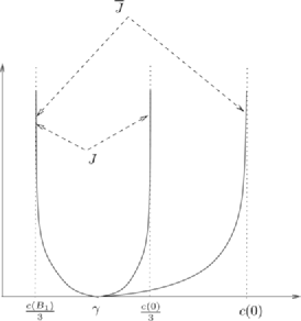
Figure 2: The rate functions $J$ and $\overline{J}$.

Unlike it may appear, we shall not prove Theorem 1.3 by first computing the Laplace transform of $\rho_{n}$ and $\overline{\rho}_{n}$ and then applying the Gärtner–Ellis theorem (see, e.g., Theorem 2.3.6 in dembo ). We shall follow another route. First, we combine Sanov’s theorem (see, e.g., Theorem 6.2.10 in dembo ) and the contraction principle (see, e.g., Theorem 4.2.1 in dembo ) to prove that the sequences $\{\rho_{n}/n\}_{n\geq 1}$ and $\{\overline{\rho}_{n}/n\}_{n\geq 1}$ obey a LDP, with rate functions given in variational form. Then, we provide the explicit expression of the rate functions solving the related variational problems. It is worthwhile to remark that, using Theorem 1.3 and Varadhan’s lemma (see, e.g., Theorem 4.3.1 in dembo ) it is easily seen that

$$\lim_{n\to\infty}\frac{1}{n}\log\mathrm{E}[{e}^{\theta\rho_{n}}]=J^{*}(\theta)\quad\mbox{and}\quad\lim_{n\to\infty}\frac{1}{n}\log\mathrm{E}[{e}^{\theta\overline{\rho}_{n}}]=\overline{J}{}^{*}(\theta)\qquad\forall\theta\in\mathbb{R},$$

where $J^{*}$ and $\overline{J}{}^{*}$ are the Fenchel–Legendre transforms of $J$ and $\overline{J}$, respectively. A nice consequence of Theorems 1.1 and 1.2 is that, in terms of law of the large numbers and central limit theorem, $\rho_{n}$ has the same asymptotic behavior as

$$\breve{\rho}_{n}=\frac{1}{3}\sum_{l=1}^{3}\sum_{k=1}^{n}\mathbh{1}\{X_{k}\in\mathbb{T}_{l}\}c_{l}(X_{k}).$$

Moreover, if the cost function satisfies extra regularity assumptions (see Proposition 4.4), by Theorem 1.3 and the Gärtner–Ellis theorem, we have that $\rho_{n}$ and $\breve{\rho}_{n}$ have the same asymptotic behavior even in terms of large deviations.

As can be seen from the proofs, if the left-hand side of assumption (1) does not hold, then we have an explicit rate function $J(y)$ only for $y<c(0)/3$. If the right-hand side of assumption (1) also fails to hold, then we have an explicit rate function $J(y)$ only for $y<y_{0}$ for some $y_{0}>\gamma$. We also point out that the statements of Theorems 1.2 and 1.3 concerning $\overline{\rho}_{n}$ do not require the use of (1) and (1).

In wireless communication, the typical cost function is the inverse of signal to noise plus interference ratio (see, e.g., Chapter IV in Tse and Viswanath tse ), which has the following shape:

$$c(x)=\frac{a+\min\{b,|x-B_{2}|^{-\alpha}\}+\min\{b,|x-B_{3}|^{-\alpha}\}}{\min\{b,|x-B_{1}|^{-\alpha}\}},\qquad x\in\mathbb{T},$$

where $\alpha\geq 2$, $a>0$ and $b>(\lambda\sqrt{3}/2)^{-\alpha}$ [recall that $\lambda=2(3\sqrt{3})^{-1/2}$ and $\lambda\sqrt{3}=|B_{1}-B_{2}|$]. We shall check in the Appendix that this cost function satisfies (1), (1), (5), (6) and (1). Moreover, the first inequality in (1) will be checked numerically and, for arbitrarily fixed $\alpha>2$ and $a>0$, we shall determine values of the parameter $b>(\lambda\sqrt{3}/2)^{-\alpha}$ such that the second inequality in (1) holds.

The remainder of the paper is organized as follows. In Section 2 we analyze the sample path properties of the optimal allocation and we prove Theorem 1.1. In Section 3 we show Theorem 1.2. Section 4 is devoted to the proof of Theorem 1.3 and Proposition 1.4. In Section 5, we discuss some generalizations of the model. We include also an Appendix where we prove some technical lemmas and provide an illustrative example.

2 Sample path properties

2.1 Structural properties of the optimal allocation

Throughout this paper we denote by $\mathcal{M}_{b}(\mathbb{T})$ the space of Borel measures on $\mathbb{T}$ with total mass less than or equal to $1$ and by $\mathcal{M}_{1}(\mathbb{T})$ the space of probability measures on $\mathbb{T}$. These spaces are both equipped with the topology of weak convergence (see, e.g., Billingsley billingsley ). For a Borel function $h$ and a Borel measure $\mu$ on $\mathbb{T}$, we set $\mu(h)=\int_{\mathbb{T}}h(x)\mu(dx)$. Consider the functional from $\mathcal{M}_{b}(\mathbb{T})^{3}$ to $\mathbb{R}$ defined by

$$\phi(\alpha_{1},\alpha_{2},\alpha_{3})=\max(\alpha_{1}(c_{1}),\alpha_{2}(c_{2}),\alpha_{3}(c_{3})).$$ (14)

Letting $\alpha_{|B}$ denote the restriction of a measure $\alpha$ to a Borel set $B$, we define the functionals $\Phi$ and $\Psi$ from $\mathcal{M}_{1}(\mathbb{T})$ to $\mathbb{R}$ by

$$\Phi(\alpha)=\inf_{(\alpha_{l})_{1\leq l\leq 3}\in\mathcal{M}_{b}(\mathbb{T})^{3}\dvtx\alpha_{1}+\alpha_{2}+\alpha_{3}=\alpha}\phi(\alpha_{1},\alpha_{2},\alpha_{3})$$

and

$$\Psi(\alpha)=\phi(\alpha_{|\mathbb{T}_{1}},\alpha_{|\mathbb{T}_{2}},\alpha_{|\mathbb{T}_{3}}).$$

Note that if $\delta_{x}$ denotes the Dirac measure with total mass at $x\in\mathbb{T}$, then

$$\frac{\overline{\rho}_{n}}{n}=\Psi\Biggl{(}\frac{1}{n}\sum_{k=1}^{n}\delta_{X_{k}}\Biggr{)}.$$ (15)

Lemma 2.1

Under assumption (6) we have that $\phi$ is continuous on $\mathcal{M}_{b}(\mathbb{T})^{3}$ and $\Psi$ and $\Phi$ are continuous on $\mathcal{M}_{1}(\mathbb{T})$ $($for the topology of the weak convergence$)$.

The proof of Lemma 2.1 is postponed to the Appendix; the continuity of $\phi$ and $\Psi$ is essentially trivial, but the continuity of $\Phi$ requires more work. Define the set of matrices

$$\mathcal{B}_{n}=\{B=(b_{kl})_{1\leq k\leq n,1\leq l\leq 3}\dvtx b_{kl}\in[0,1],b_{k1}+b_{k2}+b_{k3}=1\}$$

and

$$\widetilde{\rho}_{n}=\min_{B\in\mathcal{B}_{n}}\rho_{n}(B).$$

From the viewpoint of linear programming, this is the fractional relaxation of the original optimization problem. Now, given a matrix $B=(b_{kl})\in\mathcal{B}_{n}$, we define the associated measures $(\alpha_{1},\alpha_{2},\alpha_{3})\in\mathcal{M}_{b}(\mathbb{T})^{3}$ by setting $\alpha_{l}=(1/n)\sum_{k=1}^{n}b_{kl}\delta_{X_{k}}$ ($l=1,2,3$). Due to this correspondence, it is straightforward to check that

$$\frac{\widetilde{\rho}_{n}}{n}=\Phi\Biggl{(}\frac{1}{n}\sum_{k=1}^{n}\delta_{X_{k}}\Biggr{)}.$$ (16)

The next lemma is a collection of elementary statements, whose proofs are given in the Appendix.

Lemma 2.2

Fix $n\geq 1$ and let $B^{*}=(b^{*}_{kl})\in\mathcal{B}_{n}$ be an optimal allocation matrix for $\widetilde{\rho}_{n}$. Then:

For all $\alpha\in\mathcal{M}_{1}(\mathbb{T})$, there exists $(\alpha_{1},\alpha_{2},\alpha_{3})\in\mathcal{M}_{b}(\mathbb{T})^{3}$ such that $\alpha=\alpha_{1}+\alpha_{2}+\alpha_{3}$ and $\Phi(\alpha)=\phi(\alpha_{1},\alpha_{2},\alpha_{3})$. Moreover, whenever such equality holds, we have $\alpha_{1}(c_{1})=\alpha_{2}(c_{2})=\alpha_{3}(c_{3})$. In particular, the choice $\alpha_{l}=(1/n)\sum_{k=1}^{n}b^{*}_{kl}\delta_{X_{k}}$ $(l=1,2,3)$ yields

$$\sum_{k=1}^{n}b^{*}_{k1}c_{1}(X_{k})=\sum_{k=1}^{n}b^{*}_{k2}c_{2}(X_{k})=\sum_{k=1}^{n}b^{*}_{k3}c_{3}(X_{k}).$$

If assumption (5) holds, then

$$\rho_{n}-3\|c\|_{\infty}\leq\widetilde{\rho}_{n}\leq\rho_{n}\qquad\mbox{a.s.}$$

If assumption (5) holds then the sequences $\{\widetilde{\rho}_{n}/n\}$ and $\{\rho_{n}/n\}$ are exponentially equivalent.

For the definition of exponential equivalence, see page 130 in dembo .

2.2 Proof of Theorem 1.1

The law of large numbers yields, for all $l=1,2,3$,

$$\lim_{n\to\infty}\frac{1}{n}\sum_{k=1}^{n}c_{l}(X_{k})\mathbh{1}\{X_{k}\in\mathbb{T}_{l}\}=\int_{\mathbb{T}_{l}}c_{l}(x)\,dx=\gamma\qquad\mbox{a.s.}$$

Therefore from the identity

$$\frac{\overline{\rho}_{n}}{n}=\max_{1\leq l\leq 3}\frac{1}{n}\sum_{k=1}^{n}c_{l}(X_{k})\mathbh{1}\{X_{k}\in\mathbb{T}_{l}\},$$

we get $\lim_{n\to\infty}\overline{\rho}_{n}/n=\gamma$ a.s. We also have to prove that $\lim_{n\to\infty}\rho_{n}/n=\gamma$ a.s. Let $A=(a_{kl})\in\mathcal{A}_{n}$ be an allocation matrix. By assumption (1), if $x\in\mathbb{T}_{l}$ then $c_{l}(x)=\min_{1\leq m\leq 3}c_{m}(x)$. Therefore

$$3\rho_{n}(A) \geq \sum_{l=1}^{3}\sum_{k=1}^{n}a_{kl}c_{l}(X_{k})$$

$$\geq \sum_{l=1}^{3}\sum_{X_{k}\in\mathbb{T}_{l}}c_{l}(X_{k})$$

$$\geq 3\min_{1\leq l\leq 3}\Biggl{(}\sum_{k=1}^{n}c_{l}(X_{k})\mathbh{1}\{X_{k}\in\mathbb{T}_{l}\}\Biggr{)}.$$

So taking the minimum over all the allocation matrices we deduce

$$\min_{1\leq l\leq 3}\Biggl{(}\sum_{k=1}^{n}c_{l}(X_{k})\mathbh{1}\{X_{k}\in\mathbb{T}_{l}\}\Biggr{)}\leq\rho_{n}\leq\overline{\rho}_{n}.$$

Thus by applying the law of large numbers, we have a.s.

$$\gamma\leq\liminf_{n\to\infty}\frac{\rho_{n}}{n}\leq\limsup_{n\to\infty}\frac{\rho_{n}}{n}\leq\gamma.$$

Remark 2.3.

Assume that conditions (1), (5) and (6) hold. By Theorem 1.1 we have $\lim_{n\to\infty}\overline{\rho}_{n}/n=\gamma$ a.s. So by Lemma 2.1, equation (15) and the a.s. weak convergence of $(1/n)\sum_{k=1}^{n}\delta_{X_{k}}$ to $\ell$ we get $\Psi(\ell)=\gamma$. Similarly, using (16) in place of (15), we deduce that $\lim_{n\to\infty}\widetilde{\rho}_{n}/n=\Phi(\ell)$ a.s. By Lemma 2.2(ii), $|\widetilde{\rho}_{n}/n-\rho_{n}/n|\leq 3\|c\|_{\infty}/n$, so we obtain $\lim_{n\to\infty}\rho_{n}/n=\Phi(\ell)$ a.s., and by Theorem 1.1 we have $\Phi(\ell)=\gamma$.

3 Proof of Theorem 1.2

Consider the random signed measure

$$W_{n}=\sqrt{n}(\mu_{n}-\ell)\qquad\mbox{where }\mu_{n}=\frac{1}{n}\sum_{k=1}^{n}\delta_{X_{k}}.$$

The standard Brownian bridge $W$ on $\mathbb{T}$ is a random signed measure specified by the centered Gaussian process $\{W(f)\}$ (indexed on the set of square integrable functions on $\mathbb{T}$, with respect to $\ell$), with covariance given by

$$\mathrm{E}[W(f)W(g)]=\ell(fg)-\ell(f)\ell(g)$$

(see, e.g., Dudley dudley ). By construction,

$$\overline{\rho}_{n}=n\max_{1\leq l\leq 3}\biggl{(}\int_{\mathbb{T}_{l}}c_{l}(x)\mu_{n}(dx)\biggr{)}$$

or equivalently

$$\frac{\overline{\rho}_{n}-n\gamma}{\sqrt{n}}=\max_{1\leq l\leq 3}\biggl{(}\int_{\mathbb{T}_{l}}c_{l}(x)W_{n}(dx)\biggr{)}.$$ (18)

Let $f$ be a square integrable function on $\mathbb{T}$. Then, as $n\to\infty$,

$$W_{n}(f)=\frac{\sum_{k=1}^{n}f(X_{k})-n\ell(f)}{\sqrt{n}}\stackrel{{\scriptstyle d}}{{\rightarrow}}W(f).$$

Indeed, by the central limit theorem $W_{n}(f)$ converges in distribution to a Gaussian r.v. with zero mean and variance equal to $\ell(f^{2})-\ell^{2}(f)$, which is exactly the law of $W(f)$. Using the Lévy continuity theorem and the inversion theorem (see, e.g., Theorems 7.5 and 7.6 in billingsley ), we have, for all square integrable functions $f_{1}$, $f_{2}$ and $f_{3}$,

$$(W_{n}(f_{1}),W_{n}(f_{2}),W_{n}(f_{3}))\stackrel{{\scriptstyle d}}{{\rightarrow}}(W(f_{1}),W(f_{2}),W(f_{3})).$$

For $(x_{1},x_{2},x_{3})\in\mathbb{R}^{3}$, the function $(x_{1},x_{2},x_{3})\mapsto\max(x_{1},x_{2},x_{3})$ is continuous. Therefore, by the continuous mapping theorem (see, e.g., Theorem 5.1 in billingsley ) and (18) we have, as $n$ goes to infinity,

$$\frac{\overline{\rho}_{n}-n\gamma}{\sqrt{n}}\stackrel{{\scriptstyle d}}{{\rightarrow}}\max_{1\leq l\leq 3}\biggl{(}\int_{\mathbb{T}_{l}}c_{l}(x)W(dx)\biggr{)}.$$ (19)

We shall show later on that the r.v. in the right-hand side of (19) has the claimed distribution. Now we consider the optimal load $\rho_{n}$. By the second inequality in (2.2) we have

$$3\rho_{n}\geq n\sum_{l=1}^{3}\int_{\mathbb{T}_{l}}c_{l}(x)\mu_{n}(dx)$$

and therefore

$$3\frac{\rho_{n}-n\gamma}{\sqrt{n}}\geq\sum_{l=1}^{3}\int_{\mathbb{T}_{l}}c_{l}(x)W_{n}(dx).$$ (20)

The following proposition is the heart of the proof. It will be shown later on.

Proposition 3.1

Under the assumptions of Theorem 1.2, there exist absolute constants $L_{0}$ and $L_{1}$, not depending on $n$, such that the following holds. For any $1/4<\alpha<1/2$, with probability at least $1-L_{1}\exp(-L_{0}n^{1-2\alpha})$, there exists an allocation matrix $\hat{A}=(\hat{a}_{kl})_{1\leq k\leq n,1\leq l\leq 3}\in\mathcal{A}_{n}$ with associated load $\hat{\rho}_{n}=\rho_{n}(\hat{A})$ such that

$$\Biggl{|}3\frac{\hat{\rho}_{n}-n\gamma}{\sqrt{n}}-\sum_{l=1}^{3}\int_{\mathbb{T}_{l}}c_{l}(x)W_{n}(dx)\Biggr{|}\leq n^{1/2-2\alpha}.$$

Using this result, $\hat{\rho}_{n}\geq\rho_{n}$ and (20), we have that with probability at least $1-L_{1}\exp(-L_{0}n^{1-2\alpha})$

$$\Biggl{|}3\frac{\rho_{n}-n\gamma}{\sqrt{n}}-\sum_{l=1}^{3}\int_{\mathbb{T}_{l}}c_{l}(x)W_{n}(dx)\Biggr{|}\leq n^{1/2-2\alpha}.$$ (21)

Therefore, as $n$ goes to infinity,

$$\frac{\rho_{n}-n\gamma}{\sqrt{n}}-\frac{1}{3}\sum_{l=1}^{3}\int_{\mathbb{T}_{l}}c_{l}(x)W_{n}(dx)\stackrel{{\scriptstyle d}}{{\rightarrow}}0.$$

The continuous mapping theorem yields

$$\sum_{l=1}^{3}\int_{\mathbb{T}_{l}}c_{l}(x)W_{n}(dx)\stackrel{{\scriptstyle d}}{{\rightarrow}}\sum_{l=1}^{3}\int_{\mathbb{T}_{l}}c_{l}(x)W(dx).$$

So combining these latter two limits we get, as $n$ goes to infinity,

$$\frac{\rho_{n}-n\gamma}{\sqrt{n}}\stackrel{{\scriptstyle d}}{{\rightarrow}}\frac{1}{3}\sum_{l=1}^{3}\int_{\mathbb{T}_{l}}c_{l}(x)W(dx),$$

that is, $n^{-1/2}(\rho_{n}-n\gamma)$ converges weakly to a centered Gaussian random variable with variance $\sigma^{2}/3-\gamma^{2}$. We have considered so far, the normalized sequences $\rho_{n}$ and $\overline{\rho}_{n}$ separately. However, we can carry the same analysis on the normalized difference $\overline{\rho}_{n}-\rho_{n}$. More precisely, by (18) we have a.s.

$$\Biggl{|}\frac{\overline{\rho}_{n}-\rho_{n}}{\sqrt{n}}-\Biggl{[}\max_{1\leq l\leq 3}\biggl{(}\int_{\mathbb{T}_{l}}c_{l}(x)W_{n}(dx)\biggr{)}-\frac{1}{3}\sum_{l=1}^{3}\int_{\mathbb{T}_{l}}c_{l}(x)W_{n}(dx)\Biggr{]}\Biggr{|}$$

$$\qquad\leq\biggl{|}\frac{\overline{\rho}_{n}-n\gamma}{\sqrt{n}}-\max_{1\leq l\leq 3}\biggl{(}\int_{\mathbb{T}_{l}}c_{l}(x)W_{n}(dx)\biggr{)}\biggr{|}$$

$$\qquad\quad{}+\Biggl{|}\frac{\rho_{n}-n\gamma}{\sqrt{n}}-\frac{1}{3}\sum_{l=1}^{3}\int_{\mathbb{T}_{l}}c_{l}(x)W_{n}(dx)\Biggr{|}$$

$$\qquad=\Biggl{|}\frac{\rho_{n}-n\gamma}{\sqrt{n}}-\frac{1}{3}\sum_{l=1}^{3}\int_{\mathbb{T}_{l}}c_{l}(x)W_{n}(dx)\Biggr{|}.$$

Thus, by (21), we obtain, with probability at least $1-L_{1}\exp(-L_{0}n^{1-2\alpha})$,

$$\Biggl{|}\frac{\overline{\rho}_{n}-\rho_{n}}{\sqrt{n}}-\Biggl{[}\max_{1\leq l\leq 3}\biggl{(}\int_{\mathbb{T}_{l}}c_{l}(x)W_{n}(dx)\biggr{)}-\frac{1}{3}\sum_{l=1}^{3}\int_{\mathbb{T}_{l}}c_{l}(x)W_{n}(dx)\Biggr{]}\Biggr{|}\leq\frac{1}{3}n^{1/2-2\alpha}.$$

Therefore, as $n\to\infty$,

$$\frac{\overline{\rho}_{n}-\rho_{n}}{\sqrt{n}}-\Biggl{[}\max_{1\leq l\leq 3}\biggl{(}\int_{\mathbb{T}_{l}}c_{l}(x)W_{n}(dx)\biggr{)}-\frac{1}{3}\sum_{l=1}^{3}\int_{\mathbb{T}_{l}}c_{l}(x)W_{n}(dx)\Biggr{]}\stackrel{{\scriptstyle d}}{{\rightarrow}}0.$$

The continuous mapping theorem yields

$$\max_{1\leq l\leq 3}\biggl{(}\int_{\mathbb{T}_{l}}c_{l}(x)W_{n}(dx)\biggr{)}-\frac{1}{3}\sum_{l=1}^{3}\int_{\mathbb{T}_{l}}c_{l}(x)W_{n}(dx)$$

$$\qquad\stackrel{{\scriptstyle d}}{{\rightarrow}}\max_{1\leq l\leq 3}\biggl{(}\int_{\mathbb{T}_{l}}c_{l}(x)W(dx)\biggr{)}-\frac{1}{3}\sum_{l=1}^{3}\int_{\mathbb{T}_{l}}c_{l}(x)W(dx)$$

and therefore, as $n\to\infty$,

$$\frac{\overline{\rho}_{n}-\rho_{n}}{\sqrt{n}}\stackrel{{\scriptstyle d}}{{\rightarrow}}\max_{1\leq l\leq 3}\biggl{(}\int_{\mathbb{T}_{l}}c_{l}(x)W(dx)\biggr{)}-\frac{1}{3}\sum_{l=1}^{3}\int_{\mathbb{T}_{l}}c_{l}(x)W(dx).$$

For $l\in\{1,2,3\}$, set

$$N_{l}=\int_{\mathbb{T}_{l}}c_{l}(x)W(dx)-\frac{1}{3}\sum_{l=1}^{3}\int_{\mathbb{T}_{l}}c_{l}(x)W(dx).$$

By definition $\{W(f)\}$ is a centered Gaussian process indexed on the set of square integrable functions; therefore $N=(N_{1},N_{2},N_{3})$ follows a multivariate Gaussian distribution with mean $0$. A simple computation shows that the covariance matrix of $N$ is

$$\frac{\sigma^{2}}{3}\pmatrix{2&-1&-1\cr-1&2&-1\cr-1&-1&2}.$$

It implies that $N$ has the same distribution as

$$\bigl{(}G_{1}-(G_{1}+G_{2}+G_{3})/3,G_{2}-(G_{1}+G_{2}+G_{3})/3,G_{3}-(G_{1}+G_{2}+G_{3})/3\bigr{)},$$

where $G_{1}$, $G_{2}$ and $G_{3}$ are independent Gaussian r.v.’s with mean $0$ and variance $\sigma^{2}$. Moreover $N$ is independent of $\frac{1}{3}\sum_{l=1}^{3}\int_{\mathbb{T}_{l}}c_{l}(x)W(dx)$, and we deduce the claimed expression for (19).

It remains to compute the asymptotic behavior of the expectation of the loads. A direct computation gives, for any $l=1,2,3$,

$$\mathrm{E}\biggl{[}\biggl{(}\int_{\mathbb{T}_{l}}c_{l}(x)W_{n}(dx)\biggr{)}^{2}\biggr{]}=\frac{\sigma^{2}}{3}-\frac{\gamma^{2}}{9n}\leq\frac{\sigma^{2}}{3}.$$

Thus the sequences $\{\int_{\mathbb{T}_{l}}c_{l}(x)W_{n}(dx)\}$ $(l=1,2,3)$ are uniformly integrable. This implies that the sequence $\{\max_{1\leq l\leq 3}(\int_{\mathbb{T}_{l}}c_{l}(x)W_{n}(dx))\}$ is uniformly integrable and so using (18) we have

$$\lim_{n\to\infty}\mathrm{E}[\overline{\rho}_{n}-n\gamma]/\sqrt{n} = \lim_{n\to\infty}\mathrm{E}\biggl{[}\max_{1\leq l\leq 3}\biggl{(}\int_{\mathbb{T}_{l}}c_{l}(x)W_{n}(dx)\biggr{)}\biggr{]}$$

$$= \mathrm{E}\biggl{[}\max_{1\leq l\leq 3}\biggl{(}\int_{\mathbb{T}_{l}}c_{l}(x)W(dx)\biggr{)}\biggr{]}$$

$$= m=\mathrm{E}[\max\{G_{1},G_{2},G_{3}\}].$$

Now we give the asymptotic behavior of $\mathrm{E}[\rho_{n}]$. Note that by (21) we have

$$\mathrm{E}\Biggl{[}\Biggl{|}3\frac{\rho_{n}-n\gamma}{\sqrt{n}}-\sum_{l=1}^{3}\int_{\mathbb{T}_{l}}c_{l}(x)W_{n}(dx)\Biggr{|}\Biggr{]}$$

$$\qquad\leq n^{1/2-2\alpha}+\mathrm{E}\Biggl{[}\Biggl{|}3\frac{\rho_{n}-n\gamma}{\sqrt{n}}-\sum_{l=1}^{3}\int_{\mathbb{T}_{l}}c_{l}(x)W_{n}(dx)\Biggr{|}\mathbh{1}\{|\cdots|>n^{1/2-2\alpha}\}\Biggr{]}$$

$$\qquad\leq n^{1/2-2\alpha}+10\|c\|_{\infty}L_{1}\sqrt{n}\exp(-L_{0}n^{1-2\alpha})$$

$$\qquad=n^{1/2-2\alpha}+\widetilde{L}_{1}\sqrt{n}\exp(-L_{0}n^{1-2\alpha}),$$

where the latter inequality follows since $\gamma\leq\|c\|_{\infty}$, $\rho_{n}\leq\|c\|_{\infty}n$ and $|{\int_{\mathbb{T}_{l}}}c_{l}(x)\times\break W_{n}(dx)|\leq 2\|c\|_{\infty}\sqrt{n}$. Therefore, since $\mathrm{E}[\int_{\mathbb{T}_{l}}c_{l}(x)W_{n}(dx)]=0$ and $1/4<\alpha<1/2$, our computation leads to

$$\lim_{n\to\infty}\mathrm{E}[\rho_{n}-n\gamma]/\sqrt{n}=0.$$

Proof of Proposition 3.1 We start describing the allocation matrix $\hat{A}$. For $l,m\in\{1,2,3\}$ and $t\in[-\lambda\sqrt{3}/2,\lambda\sqrt{3}/2]$, denote by $B_{lm}(t)$ the point on the segment $\overline{B_{l}B_{m}}$ at distance $t+\lambda\sqrt{3}/2$ from $B_{l}$. We extend the definition of $B_{lm}(t)$ for all $t\in[-\lambda\sqrt{3},\lambda\sqrt{3}]$ by following the edges of $\mathbb{T}$. More precisely, we set

$$B_{12}(t)=\cases{B_{31}\bigl{(}\lambda\sqrt{3}+t\bigr{)},&\quad if $t\in\bigl{[}-\lambda\sqrt{3},-\lambda\sqrt{3}/2\bigr{]}$,\cr B_{23}\bigl{(}\lambda\sqrt{3}-t\bigr{)},&\quad if $t\in\bigl{[}\lambda\sqrt{3}/2,\lambda\sqrt{3}\bigr{]}$.}$$

For $l,m\in\{1,2,3\}$, $B_{lm}(t)$ is defined similarly by a circular permutation of the indices. For $\mathbf{t}=(t^{1},t^{2},t^{3})\in[-\lambda\sqrt{3},\lambda\sqrt{3}]^{3}$, let

$$C^{1}(\mathbf{t})=\{0\}\cup\bigl{(}\{z\in\mathbb{C}\dvtx z\cdot(B_{12}(t^{1}){e}^{-i\pi/2})\geq 0\}\cap\{z\in\mathbb{C}\dvtx z\cdot(B_{31}(t^{3}){e}^{i\pi/2})>0\}\bigr{)}$$

be the (possibly empty) cone delimited by the straight line determined by the points $0$, $B_{12}(t^{1})$ and $B_{31}(t^{3})$. We define $\Gamma^{1}(\mathbf{t})=C^{1}(\mathbf{t})\cap\mathbb{T}$. Similarly, let $\Gamma^{2}(\mathbf{t})=C^{2}(\mathbf{t})\cap\mathbb{T}$ and $\Gamma^{3}(\mathbf{t})=C^{3}(\mathbf{t})\cap\mathbb{T}$ with

$$C^{2}(\mathbf{t}) = \{z\in\mathbb{C}\dvtx z\cdot(B_{12}(t^{1}){e}^{i\pi/2})>0\}\cap\{z\in\mathbb{C}\dvtx z\cdot(B_{23}(t^{2}){e}^{-i\pi/2})\geq 0\},$$

$$C^{3}(\mathbf{t}) = \{z\in\mathbb{C}\dvtx z\cdot(B_{23}(t^{2}){e}^{i\pi/2})>0\}\cap\{z\in\mathbb{C}\dvtx z\cdot(B_{31}(t^{3}){e}^{-i\pi/2})\geq 0\}.$$

By construction, the sets $\Gamma^{1}(\mathbf{t})$, $\Gamma^{2}(\mathbf{t})$ and $\Gamma^{3}(\mathbf{t})$ are disjoint and their union is $\mathbb{T}$. For $l\in\{1,2,3\}$, set

$$\rho_{n}^{l}(\mathbf{t})=\sum_{k=1}^{n}c_{l}(X_{k})\mathbh{1}\{X_{k}\in\Gamma^{l}(\mathbf{t})\}$$

and consider the following recursion. At step $0$: for $\mathbf{t}_{0}=(0,0,0)$, define

$$m_{0}=\mathop{\arg\min}_{1\leq l\leq 3}\rho_{n}^{l}(\mathbf{t}_{0})$$

(breaking ties with the lexicographic order) and

$$M_{0}=\mathop{\arg\max}_{1\leq l\leq 3}\rho_{n}^{l}(\mathbf{t}_{0})$$

(again breaking ties with the lexicographic order). If $\rho_{n}^{M_{0}}(\mathbf{t}_{0})-\rho_{n}^{m_{0}}(\mathbf{t}_{0})\leq 2\|c\|_{\infty}$, the recursion stops. Otherwise, $\rho_{n}^{M_{0}}(\mathbf{t}_{0})-\rho_{n}^{m_{0}}(\mathbf{t}_{0})>2\|c\|_{\infty}$ and there is at least one point $X_{i}$ $(i=1,\ldots,n)$ in $\Gamma^{M_{0}}(\mathbf{t}_{0})$. Note also that, a.s., for all $\theta\in[0,2\pi]$, there is at most one point of $\{X_{1},\ldots,X_{n}\}$ on the straight line $(x{e}^{i\theta},x>0)$. As a consequence there exists a random variable $0\leq t_{1}\leq\lambda\sqrt{3}$ such that, a.s., there is exactly one point $X_{i}$ $(i=1,\ldots,n)$ in the triangle with vertices $\{0,B_{m_{0}M_{0}}(t_{1}),B_{m_{0}M_{0}}(0)\}$ for $0\leq t_{1}\leq\lambda\sqrt{3}/2$, or in the polygon with vertices $\{0,B_{m_{0}M_{0}}(t_{1}),B_{M_{0}},B_{m_{0}M_{0}}(0)\}$ for $\lambda\sqrt{3}/2<t_{1}\leq\lambda\sqrt{3}$. We then set $\mathbf{t}_{1}=(t_{1}^{1},t_{1}^{2},t_{1}^{3}):=(t_{1},0,0)$ if $m_{0}=1$, $M_{0}=2$; $\mathbf{t}_{1}=(-t_{1},0,0)$ if $m_{0}=2$, $M_{0}=1$; $\mathbf{t}_{1}=(0,t_{1},0)$ if $m_{0}=2$, $M_{0}=3$; $\mathbf{t}_{1}=(0,-t_{1},0)$ if $m_{0}=3$, $M_{0}=2$; $\mathbf{t}_{1}=(0,0,-t_{1})$ if $m_{0}=1$, $M_{0}=3$; $\mathbf{t}_{1}=(0,0,t_{1})$ if $m_{0}=3$, $M_{0}=1$. The sets $(\Gamma^{1}(\mathbf{t}_{1}),\Gamma^{2}(\mathbf{t}_{1}),\Gamma^{3}(\mathbf{t}_{1}))$ are thus designed to allocate one extra point to bin $m_{0}$ and one less to $M_{0}$. By construction, we have

$$\rho_{n}^{m_{0}}(\mathbf{t}_{1})<\rho_{n}^{M_{0}}(\mathbf{t}_{1}),\qquad\max_{1\leq l\leq 3}\rho_{n}^{l}(\mathbf{t}_{1})<\max_{1\leq l\leq 3}\rho_{n}^{l}(\mathbf{t}_{0})$$

and

$$\min_{1\leq l\leq 3}\rho_{n}^{l}(\mathbf{t}_{1})>\min_{1\leq l\leq 3}\rho_{n}^{l}(\mathbf{t}_{0}).$$

At step 1: define

$$m_{1}=\mathop{\arg\min}_{1\leq l\leq 3}\rho_{n}^{l}(\mathbf{t}_{1})$$

(breaking ties with the lexicographic order) and

$$M_{1}=\mathop{\arg\max}_{1\leq l\leq 3}\rho_{n}^{l}(\mathbf{t}_{1})$$

(again breaking ties with the lexicographic order). Similarly to step $0$, if $\rho_{n}^{M_{1}}(\mathbf{t}_{1})-\rho_{n}^{m_{1}}(\mathbf{t}_{1})>2\|c\|_{\infty}$, then there is at least one point of $\{X_{1},\ldots,X_{n}\}$ in $\Gamma^{M_{1}}(\mathbf{t}_{1})$ and we build the random vector $\mathbf{t}_{2}=(t_{2}^{1},t_{2}^{2},t_{2}^{3})$ in order to allocate one extra point to bin $m_{1}$ and one less to $M_{1}$. The recursion stops at the first step $k\geq 0$ such that

$$\rho_{n}^{M_{k}}(\mathbf{t}_{k})-\rho_{n}^{m_{k}}(\mathbf{t}_{k})\leq 2\|c\|_{\infty}$$

(where $m_{k}$, $M_{k}$ and $\mathbf{t}_{k}$ are defined similarly to $m_{0},m_{1},\ldots,M_{0},M_{1},\ldots$ and $\mathbf{t}_{1},\mathbf{t}_{2},\ldots$). As we shall check soon, the recursion stops after at most $n$ steps. When the recursion stops, say at step $k_{n}\leq n$, we set $\Gamma^{l}_{n}=\Gamma^{l}(\mathbf{t}_{k_{n}})$ and $\mathbf{t}_{n}=\mathbf{t}_{k_{n}}$. The allocation matrix $\hat{A}$ is defined by allocating $X_{k}$ to the bin in $B_{l}$ if $X_{k}\in\Gamma^{l}_{n}$, that is,

$$\hat{A}=(\hat{a}_{kl})_{1\leq k\leq n,1\leq l\leq 3}\qquad\mbox{where }\hat{a}_{kl}=\mathbh{1}\{X_{k}\in\Gamma_{n}^{l}\}.$$

By construction, we have for all $l,m\in\{1,2,3\}$,

$$|\rho^{l}_{n}(\mathbf{t}_{n})-\rho^{m}_{n}(\mathbf{t}_{n})|\leq 2\|c\|_{\infty}.$$ (22)

We now analyze the recursion more closely. Assume that at step $0$ we have $m_{0}=3$ and $M_{0}=1$, that is, $\rho^{1}_{n}(\mathbf{t}_{0})\geq\rho^{2}_{n}(\mathbf{t}_{0})\geq\rho^{3}_{n}(\mathbf{t}_{0})$. Then, for all $k\leq k_{n}$,

$$\rho^{1}_{n}(\mathbf{t}_{k})\geq\rho^{2}_{n}(\mathbf{t}_{k})-\|c\|_{\infty}\quad\mbox{and}\quad\rho^{3}_{n}(\mathbf{t}_{k})\leq\rho^{2}_{n}(\mathbf{t}_{k})+\|c\|_{\infty}.$$ (23)

Indeed, if for all $k<k_{n}$, $m_{k}=3$ and $M_{k}=1$, there is nothing to prove since $|\rho^{l}_{n}(\mathbf{t}_{k+1})-\rho^{l}_{n}(\mathbf{t}_{k})|\leq\|c\|_{\infty}$. Assume that there exists $k<k_{n}$ such that $m_{k}\neq 3$ or $M_{k}\neq 1$. We define

$$k_{0}=\min\{k\geq 1\dvtx m_{k}\neq 3\mbox{ or }M_{k}\neq 1\}.$$

For concreteness, assume, for example, that $M_{k_{0}}\neq 1$. By construction, $k_{0}-1<k_{n}$ so that $\rho_{n}^{1}(\mathbf{t}_{k_{0}-1})>\rho_{n}^{3}(\mathbf{t}_{k_{0}-1})+2\|c\|_{\infty}$. Since $\rho_{n}^{1}(\mathbf{t}_{k_{0}-1})\geq\rho_{n}^{2}(\mathbf{t}_{k_{0}-1})\geq\rho_{n}^{3}(\mathbf{t}_{k_{0}-1})$, we deduce that $M_{k_{0}}=2$ and $m_{k_{0}}=3$. Recall that, for $k<k_{n}$, $\rho_{n}^{M_{k}}(\mathbf{t}_{k})-\|c\|_{\infty}\leq\rho_{n}^{M_{k}}(\mathbf{t}_{k+1})<\rho_{n}^{M_{k}}(\mathbf{t}_{k})$. Thus, for $k=k_{0}-1$, from $\rho^{1}_{n}(\mathbf{t}_{k_{0}})\leq\rho^{2}_{n}(\mathbf{t}_{k_{0}})=\rho^{2}_{n}(\mathbf{t}_{k_{0}-1})\leq\rho^{1}_{n}(\mathbf{t}_{k_{0}-1})$, we obtain

$$\rho_{n}^{2}(\mathbf{t}_{k_{0}})-\|c\|_{\infty}\leq\rho_{n}^{1}(\mathbf{t}_{k_{0}}).$$

Similarly, for $k<k_{n}$, $\rho_{n}^{m_{k}}(\mathbf{t}_{k})+\|c\|_{\infty}\geq\rho_{n}^{m_{k}}(\mathbf{t}_{k+1})>\rho_{n}^{m_{k}}(\mathbf{t}_{k})$. Thus, from $\rho^{3}_{n}(\mathbf{t}_{k_{0}-1})\leq\rho^{2}_{n}(\mathbf{t}_{k_{0}})=\rho^{2}_{n}(\mathbf{t}_{k_{0}-1})$, we have

$$\rho_{n}^{3}(\mathbf{t}_{k_{0}})\leq\|c\|_{\infty}+\rho_{n}^{2}(\mathbf{t}_{k_{0}}).$$

We have proved so far that the inequalities in (23) hold for all $k\leq k_{0}$. Since $|\rho^{l}_{n}(\mathbf{t}_{k+1})-\rho^{l}_{n}(\mathbf{t}_{k})|\leq\|c\|_{\infty}$ and $\rho^{1}_{n}(\mathbf{t}_{k_{0}-1})-\rho^{3}_{n}(\mathbf{t}_{k_{0}-1})>2\|c\|_{\infty}$ we get

$$\rho^{1}_{n}(\mathbf{t}_{k_{0}})-\rho^{3}_{n}(\mathbf{t}_{k_{0}})>0.$$

Thus $m_{k_{0}}=3$ and $\rho_{n}^{3}(\mathbf{t}_{k_{0}})\leq\rho_{n}^{1}(\mathbf{t}_{k_{0}})\leq\rho_{n}^{2}(\mathbf{t}_{k_{0}})$. Define

$$k_{1}=\min\bigl{\{}k_{n},\min\{k>k_{0}\dvtx m_{k}\neq 3\mbox{ or }M_{k}\neq 2\}\bigr{\}}.$$

For $k=k_{0},\ldots,k_{1}-1$, $\rho^{2}_{n}(\mathbf{t}_{k+1})<\rho^{2}_{n}(\mathbf{t}_{k})$ and $\rho^{1}_{n}(\mathbf{t}_{k+1})=\rho^{1}_{n}(\mathbf{t}_{k})$ is constant, so the left-hand side inequality of (23) holds. Also, since $k_{1}\leq k_{n}$, for $k\in\{k_{0}+1,\ldots,k_{1}-1\}$, $\rho^{3}_{n}(\mathbf{t}_{k})<\rho^{2}_{n}(\mathbf{t}_{k})+4\|c\|_{\infty}$. So finally, (23) holds for $k=0,\ldots,k_{1}$. Moreover, if $k_{1}<k_{n}$, then $M_{k_{1}}=1$ and $m_{k_{1}}=3$. Indeed, as above, $\rho_{n}^{2}(\mathbf{t}_{k_{1}-1})-\rho_{n}^{3}(\mathbf{t}_{k_{1}-1})>2\|c\|_{\infty}$ implies

$$\rho_{n}^{2}(\mathbf{t}_{k_{1}})>\rho_{n}^{3}(\mathbf{t}_{k_{1}}).$$

So $M_{k_{1}}\neq 3$ and $m_{k_{1}}\neq 2$. If $m_{k_{1}}=1$ and $M_{k_{1}}=2$, then we write, by (23),

$$\rho_{n}^{1}(\mathbf{t}_{k_{1}})+\|c\|_{\infty}\geq\rho_{n}^{2}(\mathbf{t}_{k_{1}})>\rho_{n}^{3}(\mathbf{t}_{k_{1}})\geq\rho_{n}^{1}(\mathbf{t}_{k_{1}}).$$

So $k_{1}=k_{n}$, a contradiction. Therefore, we necessarily have $M_{k_{1}}=1$ and $m_{k_{1}}=3$. By recursion, it shows that for all $k<k_{n}$, $m_{k}=3$. Hence, at each step one point is added to the bin at $B_{3}$. No point is added to the bins at $B_{1}$ and $B_{2}$, points may only be removed from the bins at $B_{1}$ and $B_{2}$. Since there are at most $n$ points, we deduce $k_{n}\leq n$, as claimed. Also, since $\Gamma^{l}(\mathbf{t}_{0})=\mathbb{T}_{l}$, we obtain, for all $k=1,\ldots,k_{n}$, $\mathbb{T}_{3}\subset\Gamma^{3}(\mathbf{t}_{k})$, $\mathbb{T}_{2}\supseteq\Gamma^{2}(\mathbf{t}_{k})$ and $\mathbb{T}_{1}\supset\Gamma^{1}(\mathbf{t}_{k})$. The other case, where $m_{k_{0}}=2$ could be treated similarly. So more generally, if, at some step, $l=m_{k}$ then $l\neq M_{j}$ for all $k<j<k_{n}$, and conversely, if $l=M_{k}$ then $l\neq m_{j}$ for all $k<j<k_{n}$. It implies that $\Gamma^{l}(\mathbf{t}_{k})$ is a monotone sequence in $k$. Since $\Gamma^{l}(\mathbf{t}_{0})=\mathbb{T}_{l}$, for all $l\in\{1,2,3\}$,

$$\Gamma^{l}_{n}\subseteq\mathbb{T}_{l}\quad\mbox{or}\quad\mathbb{T}_{l}\subseteq\Gamma^{l}_{n}.$$ (24)

Assume now, that $t^{1}_{n}>zn^{-\alpha}$ with $z>0$ then, from (24), $\mathbb{T}_{1}\subseteq\Gamma^{1}_{n}$ and $\Gamma^{2}_{n}\subseteq\mathbb{T}_{2}$. For $t\in\mathbb{R}$, define the set $V^{1}(t)=\Gamma^{1}(t,0,0)\setminus\mathbb{T}_{1}$. On the event $\{t_{n}^{1}>zn^{-\alpha}\}$ we have

$$\rho_{n}^{1}(\mathbf{t}_{n})\geq n\int_{\mathbb{T}_{1}}c(x)\mu_{n}(dx)+n\int_{V^{1}(zn^{-\alpha})}c(x)\mu_{n}(dx)$$

and

$$\rho_{n}^{2}(\mathbf{t}_{n})\leq n\int_{\mathbb{T}_{2}}c_{2}(x)\mu_{n}(dx).$$

So, by inequality (22), we deduce that on $\{t_{n}^{1}>zn^{-\alpha}\}$

$$\int_{\mathbb{T}_{1}}c(x)\mu_{n}(dx)+\int_{V^{1}(zn^{-\alpha})}c(x)\mu_{n}(dx)\leq\int_{\mathbb{T}_{2}}c_{2}(x)\mu_{n}(dx)+\frac{2\|c\|_{\infty}}{n}.$$

Or, equivalently,

$$\quad\{t_{n}^{1}>zn^{-\alpha}\} \subseteq \biggl{\{}\sqrt{n}\int_{V^{1}(zn^{-\alpha})}c(x)\mu_{n}(dx)$$

$$\hskip 5.7pt\leq\int_{\mathbb{T}_{2}}c_{2}(x)W_{n}(dx)-\int_{\mathbb{T}_{1}}c(x)W_{n}(dx)+\frac{2\|c\|_{\infty}}{\sqrt{n}}\biggr{\}}.$$

Let $A$ be a Borel set in $\mathbb{T}$. By Hoeffding’s concentration inequality (see, e.g., Corollary 2.4.14 in dembo ) we have, for all $s\geq 0$ and $l\in\{1,2,3\}$,

$$P\biggl{(}\int_{A}c_{l}(x)\mu_{n}(dx)-\int_{A}c_{l}(x)\,dx\geq s\biggr{)} \leq \exp(-K_{0}s^{2}n),$$ (26)

$$P\biggl{(}\int_{A}c_{l}(x)\mu_{n}(dx)-\int_{A}c_{l}(x)\,dx\leq-s\biggr{)} \leq \exp(-K_{0}s^{2}n),$$ (27)

where $K_{0}=2\|c\|_{\infty}^{-2}$. Taking $s=yn^{-\alpha}$, where $y>0$, we have

$$P\biggl{(}\int_{\mathbb{T}_{l}}c_{l}(x)W_{n}(dx)\geq yn^{{1}/{2}-\alpha}\biggr{)} \leq \exp(-K_{0}y^{2}n^{1-2\alpha}),$$

$$P\biggl{(}\int_{\mathbb{T}_{l}}c_{l}(x)W_{n}(dx)\leq-yn^{{1}/{2}-\alpha}\biggr{)} \leq \exp(-K_{0}y^{2}n^{1-2\alpha}).$$

Similarly, by (27) we deduce, for $s\geq 0$,

$$P\biggl{(}\int_{V^{1}(zn^{-\alpha})}c(x)\mu_{n}(dx)\leq\int_{V^{1}(zn^{-\alpha})}c(x)\,dx-s\biggr{)}\leq\exp(-K_{0}s^{2}n).$$

By assumption (1), there exists $c_{0}>0$ such that $c(x)>c_{0}$, for all $x\in V^{1}(zn^{-\alpha})$. If $0\leq s\leq\lambda\sqrt{3}/2$, the area of $V^{1}(s)$ is equal to $\lambda s/4$. Therefore, for all $0\leq z\leq\lambda\sqrt{3}n^{\alpha}/2$,

$$K_{1}zn^{-\alpha}\leq\int_{V^{1}(zn^{-\alpha})}c(x)\,dx\leq K_{2}zn^{-\alpha}$$

with $K_{1}=c_{0}\lambda/4$ and $K_{2}=\|c\|_{\infty}\lambda/4$. So, taking $s=K_{1}zn^{-\alpha}/2$, we get, for all $0\leq z\leq\lambda\sqrt{3}n^{\alpha}$,

$$\qquad P\biggl{(}\sqrt{n}\int_{V^{1}(zn^{-\alpha})}c(x)\mu_{n}(dx)\leq\frac{K_{1}}{2}zn^{{1}/{2}-\alpha}\biggr{)}\leq\exp(-K_{3}z^{2}n^{1-2\alpha}),$$ (29)

where $K_{3}=K_{0}K_{1}^{2}/4$. Similarly, for $t\geq 0$, if $e_{1}=(1,0,0)$, $e_{2}=(0,1,0)$, $e_{3}=(0,0,1)$, we define

$$U^{l}(t)=\bigl{(}\Gamma^{l}(te_{l})\setminus\mathbb{T}_{l}\bigr{)}\cup\bigl{(}\Gamma^{l}(-te_{l})\setminus\mathbb{T}_{\sigma(l)}\bigr{)},$$

where $\sigma=(1\ 2\ 3)$ is the cyclic permutation. By (26) we have, for all $s\geq 0$,

$$P\biggl{(}\int_{U^{1}(zn^{-\alpha})}c(x)\mu_{n}(dx)\geq\int_{U^{1}(zn^{-\alpha})}c(x)\,dx+s\biggr{)}\leq\exp(-K_{0}s^{2}n).$$

Thus, setting $s=zn^{-\alpha}$, we get

$$P\bigl{(}\mu_{n}(U^{1}(zn^{-\alpha}))\geq K_{4}zn^{-\alpha}\bigr{)}\leq\exp(-K_{0}z^{2}n^{1-2\alpha})$$ (30)

with $K_{4}=1+2K_{2}$. Now, note that by (3), from the union bound, for $y>0$,

$$\{t_{n}^{1}>zn^{-\alpha}\} \subseteq \biggl{\{}\sqrt{n}\int_{V^{1}(zn^{-\alpha})}c(x)\mu_{n}(dx)\leq yn^{{1}/{2}-\alpha}\biggr{\}}$$

$${}\cup\biggl{\{}-\int_{\mathbb{T}_{1}}c_{1}(x)W_{n}(dx)+\frac{\|c\|_{\infty}}{\sqrt{n}}>\frac{1}{2}yn^{{1}/{2}-\alpha}\biggr{\}}$$

$${}\cup\biggl{\{}\int_{\mathbb{T}_{2}}c_{2}(x)W_{n}(dx)+\frac{\|c\|_{\infty}}{\sqrt{n}}>\frac{1}{2}yn^{{1}/{2}-\alpha}\biggr{\}}.$$

Now take $y=K_{1}z/2$. By (3) and (29), if $4\|c\|_{\infty}n^{\alpha-1}{K_{1}}^{-1}\leq z\leq\lambda\sqrt{3}n^{\alpha}$ we deduce

$$P(t^{1}_{n}>zn^{-\alpha}) \leq \exp(-K_{3}z^{2}n^{1-2\alpha})+2\exp\biggl{(}-\frac{K_{0}}{16}n^{1-2\alpha}(K_{1}z-4\|c\|_{\infty}n^{\alpha-1})^{2}\biggr{)}$$

$$\leq 3\exp\bigl{(}-K_{5}n^{1-2\alpha}(K_{1}z-4\|c\|_{\infty}n^{\alpha-1})^{2}\bigr{)}$$

with $K_{5}=\min\{K_{3}K_{1}^{-2},K_{0}/16\}$. Therefore, by symmetry, for all $n$ and $z>0$ such that $4\|c\|_{\infty}n^{\alpha-1}K_{1}^{-1}\leq z\leq\lambda\sqrt{3}n^{\alpha}/2$

$$P\Bigl{(}\max_{1\leq l\leq 3}|t^{l}_{n}|>zn^{-\alpha}\Bigr{)}\leq 18e^{-K_{5}n^{1-2\alpha}(K_{1}z-4\|c\|_{\infty}n^{\alpha-1})^{2}}.$$ (31)

Note that $\hat{\rho}_{n}=\rho_{n}(\hat{A})=\max_{1\leq l\leq 3}\rho_{n}^{l}(t_{n}^{l})$, so by (22) we have

$$3\hat{\rho}_{n}-4\|c\|_{\infty}\leq\rho^{1}_{n}(\mathbf{t}_{n})+\rho^{2}_{n}(\mathbf{t}_{n})+\rho^{3}_{n}(\mathbf{t}_{n})\leq 3\hat{\rho}_{n}.$$

Subtracting $3\sqrt{n}\gamma$, it follows

$$3\frac{\hat{\rho}_{n}-n\gamma}{\sqrt{n}}-\frac{4\|c\|_{\infty}}{\sqrt{n}}\leq\sqrt{n}\sum_{l=1}^{3}\biggl{(}\int_{\Gamma^{l}_{n}}c_{l}(x)\mu_{n}(dx)-\gamma\biggr{)}\leq 3\frac{\hat{\rho}_{n}-n\gamma}{\sqrt{n}}.$$

Then we subtract the quantity

$$\sum_{l=1}^{3}\int_{\mathbb{T}_{l}}c_{l}(x)W_{n}(dx)=\sqrt{n}\sum_{l=1}^{3}\biggl{(}\int_{\mathbb{T}_{l}}c_{l}(x)\mu_{n}(dx)-\gamma\biggr{)}$$

and we get

$$\Biggl{|}3\frac{\hat{\rho}_{n}-n\gamma}{\sqrt{n}}-\sum_{l=1}^{3}\int_{\mathbb{T}_{l}}c_{l}(x)W_{n}(dx)\Biggr{|}$$

$$\qquad\leq\sqrt{n}\Biggl{|}\sum_{l=1}^{3}\int_{\Gamma^{l}_{n}}c_{l}(x)\mu_{n}(dx)-\sum_{l=1}^{3}\int_{\mathbb{T}_{l}}c_{l}(x)\mu_{n}(dx)\Biggr{|}+\frac{4\|c\|_{\infty}}{\sqrt{n}}.$$

Set $c_{\min}(x)=\min(c_{1}(x),c_{2}(x),c_{3}(x))$, and note that if $x\in\mathbb{T}_{l}$ then $c_{\min}(x)=c_{l}(x)$. If $t^{l}_{n}\geq 0$, we set $V_{n}^{l}=V^{l}(t_{n}^{l})=\Gamma_{n}^{l}\setminus\mathbb{T}_{l}$, and, if $t^{l}_{n}<0$, we set $V^{l}_{n}=\Gamma_{n}^{\sigma(l)}\setminus\mathbb{T}_{l}$, where $\sigma=(1\ 2\ 3)$ is the cyclic permutation. So

$$\sum_{l=1}^{3}\int_{\Gamma^{l}_{n}}c_{l}(x)\mu_{n}(dx)-\sum_{l=1}^{3}\int_{\mathbb{T}_{l}}c_{l}(x)\mu_{n}(dx)$$

$$\qquad=\sum_{l=1}^{3}\int_{\Gamma^{l}_{n}}\bigl{(}c_{l}(x)-c_{\min}(x)\bigr{)}\mu_{n}(dx)$$

(33)

$$\qquad=\sum_{l=1}^{3}\mathbh{1}\{t_{n}^{l}\geq 0\}\int_{V^{l}_{n}}\bigl{(}c_{l}(x)-c_{\min}(x)\bigr{)}\mu_{n}(dx)$$

$$\qquad\quad{}+\sum_{l=1}^{3}\mathbh{1}\{t_{n}^{l}<0\}\int_{V^{l}_{n}}\bigl{(}c_{\sigma(l)}(x)-c_{\min}(x)\bigr{)}\mu_{n}(dx).$$

Note that if $x\in\mathbb{T}_{m}$, with $m\neq l$, then $|c_{l}(x)-c_{\min}(x)|=|c_{l}(x)-c_{m}(x)|$. For example, assume $l=1$, $m=2$ and $x=t{e}^{i{\pi}/{6}+i\theta}\in\mathbb{T}_{2}$, with $0\leq\theta\leq\pi/3$, we then have

$$|c_{1}(x)-c_{\min}(x)| = |c_{1}(x)-c_{2}(x)|=|c(t{e}^{i{\pi}/{6}+i\theta})-c(t{e}^{i{\pi}/{6}+i\theta}{e}^{-i{2\pi}/{3}})|$$

$$= |c(t{e}^{i{\pi}/{6}+i\theta})-c(t{e}^{-i{\pi}/{2}+i\theta})|.$$

By the symmetry assumption (1), we deduce

$$|c_{1}(x)-c_{\min}(x)|=|c(t{e}^{i{\pi}/{6}+i\theta})-c(t{e}^{i{\pi}/{6}-i\theta})|.$$

Again by assumption (1), $c$ is Lipschitz in a neighborhood of $D_{1}\cup D_{3}$. Letting $L>0$ denote the Lipschitz constant, if $x$ is close enough to $D_{1}$, say the distance $d(x,D_{1})$ from $x$ to $D_{1}$ is less than or equal to $\varepsilon$ with $0<\varepsilon<\lambda\sqrt{3}/2$, we have

$$|c_{1}(x)-c_{\min}(x)| \leq Lt|{e}^{i{\pi}/{6}+i\theta}-{e}^{i{\pi}/{6}-i\theta}|=Lt|{e}^{i\theta}-{e}^{-i\theta}|$$

$$= 2Lt\sin\theta=2Ld(x,D_{1}).$$

By symmetry, for all $l\in\{1,2,3\}$, if $d(x,D_{l})\leq\varepsilon$, then

$$|c_{l}(x)-c_{\min}(x)|\leq 2Ld(x,D_{l})\quad\mbox{and}\quad\bigl{|}c_{\sigma(l)}(x)-c_{\min}(x)\bigr{|}\leq 2Ld(x,D_{l}).$$

Fix $\alpha\in(1/4,1/2)$, $z>0$ and choose $n$ large enough so that $4\|c\|_{\infty}n^{\alpha-1}K_{1}^{-1}\leq z\leq\varepsilon n^{\alpha}$. Then, by (31) with probability at least $1-18e^{-K_{5}n^{1-2\alpha}(K_{1}z-4\|c\|_{\infty}n^{\alpha-1})^{2}}$, we have $\max_{1\leq l\leq 3}|t^{l}_{n}|\leq zn^{-\alpha}$. On this event, if $x\in V^{l}(t_{n}^{l})$ then $d(x,D_{l})\leq zn^{-\alpha}\leq\varepsilon$. It follows by (3) that, with probability at least $1-18\times\break e^{-K_{5}n^{1-2\alpha}(K_{1}z-4\|c\|_{\infty}n^{\alpha-1})^{2}}$,

$$\sqrt{n}\Biggl{|}\sum_{l=1}^{3}\int_{\Gamma^{l}_{n}}c_{l}(x)\mu_{n}(dx)-\sum_{l=1}^{3}\int_{\mathbb{T}_{l}}c_{l}(x)\mu_{n}(dx)\Biggr{|}$$

$$\qquad\leq\sqrt{n}\sum_{l=1}^{3}2Lzn^{-\alpha}\mu_{n}(V^{l}_{n})$$

$$\qquad\leq 2Lzn^{{1}/{2}-\alpha}\sum_{l=1}^{3}\mu_{n}(U^{l}(zn^{-\alpha})).$$

By (30), with probability at least $1-3\exp(-K_{0}z^{2}n^{1-2\alpha})$, it holds$\sum_{l=1}^{3}\mu_{n}(U^{l}(zn^{-\alpha}))\leq 3K_{4}zn^{-\alpha}$. Using that for all events $A,B$ it holds $P(A\cap B)\geq 1-P(A^{c})-P(B^{c})$, we obtain, for all $n$ large enough so that $4\|c\|_{\infty}n^{\alpha-1}\times\break K_{1}^{-1}\leq z\leq\varepsilon n^{\alpha}$,

$$\sqrt{n}\Biggl{|}\sum_{l=1}^{3}\int_{\Gamma^{l}_{n}}c_{l}(x)\mu_{n}(dx)-\sum_{l=1}^{3}\int_{\mathbb{T}_{l}}c_{l}(x)\mu_{n}(dx)\Biggr{|}\leq 12LK_{4}z^{2}n^{{1}/{2}-2\alpha}$$

with probability at least $1-21\exp(-K_{6}n^{1-2\alpha}(K_{1}z-4\|c\|_{\infty}n^{\alpha-1})^{2})$, where $K_{6}=\min\{K_{0}{K_{1}}^{-2},K_{5}\}$. By this latter inequality and (3), with the same probability,

$$\Biggl{|}3\frac{\hat{\rho}_{n}-\gamma}{\sqrt{n}}-\sum_{l=1}^{3}\int_{\mathbb{T}_{l}}c_{l}(x)W_{n}(dx)\Biggr{|}\leq 12LK_{2}z^{2}n^{{1}/{2}-2\alpha}+4\|c\|_{\infty}n^{-{1}/{2}}.$$

Fix $z=(24LK_{2})^{-{1}/{2}}$ so that $12LK_{2}z^{2}=1/2$. Then there exists $n_{0}$ such that, for all $n\geq n_{0}$, $4\|c\|_{\infty}n^{\alpha-1}K_{1}^{-1}\leq z\leq\varepsilon n^{\alpha}$ and $8\|c\|_{\infty}n^{-{1}/{2}}\leq n^{{1}/{2}-2\alpha}$. Then, for all $n\geq n_{0}$,

$$\Biggl{|}3\frac{\hat{\rho}_{n}-\gamma}{\sqrt{n}}-\sum_{l=1}^{3}\int_{\mathbb{T}_{l}}c_{l}(x)W_{n}(dx)\Biggr{|}\leq n^{1/2-2\alpha}$$ (34)

with probability at least

$$1-21\exp\bigl{(}-K_{6}n^{1-2\alpha}\bigl{(}K_{1}(24LK_{2})^{-{1}/{2}}-4\|c\|_{\infty}n_{0}^{\alpha-1}\bigr{)}^{2}\bigr{)}$$

$$\qquad=1-K_{7}\exp(-K_{8}n^{1-2\alpha}).$$

Finally, we set $L_{0}=K_{8}$ and $L_{1}=\max\{K_{7},K_{9}\}$, where $K_{9}=\exp(K_{8}n_{0}^{1-2\alpha})$. With this choice of $L_{0}$ and $L_{1}$, (34) holds for all $n\geq 1$ with probability at least $1-L_{1}\exp(-L_{0}n^{1-2\alpha})$.

4 Large deviation principles

In this section we provide LDPs for the optimal and suboptimal load. Letting $\ll$ denote absolute continuity between measures, we define by

$$H(\nu|\ell)=\cases{\displaystyle\int_{\mathbb{T}}\frac{d\nu}{d\ell}(x)\log\frac{d\nu}{d\ell}(x)\,d\ell,&\quad if $\nu\ll\ell$,\vspace*{2pt}\cr+\infty,&\quad otherwise,}$$

the relative entropy of $\nu\in\mathcal{M}_{1}(\mathbb{T})$ with respect to the Lebesgue measure $\ell$. Moreover, if $f$ is a nonnegative measurable function on $\mathbb{T}$, we denote by $\ell_{f}$ the measure on $\mathbb{T}$ with density $f$. In particular, if $\int_{\mathbb{T}}f(x)\,dx=1$, we set

$$H(f)=H(\ell_{f}|\ell)=\int_{\mathbb{T}}f(x)\log f(x)\,dx.$$

4.1 Combining Sanov’s theorem and the contraction principle

Next Theorem 4.1 follows combining Sanov’s theorem and the contraction principle.

Theorem 4.1

Assume (5) and (6). Then:

$\{\rho_{n}/n\}_{n\geq 1}$ satisfies an LDP on $\mathbb{R}$ with good rate function

$$J(y)=\inf_{\alpha\in\mathcal{M}_{1}(\mathbb{T})\dvtx\Phi(\alpha)=y}H(\alpha|\ell).$$ (35)

$\{\overline{\rho}_{n}/n\}_{n\geq 1}$ satisfies an LDP on $\mathbb{R}$ with good rate function

$$\overline{J}(y)=\inf_{\alpha\in\mathcal{M}_{1}(\mathbb{T})\dvtx\Psi(\alpha)=y}H(\alpha|\ell).$$ (36)

By Sanov’s theorem (see, e.g., Theorem 6.2.10 in dembo ) the sequence $\{\frac{1}{n}\sum_{i=1}^{n}\delta_{X_{i}}\}_{n\geq 1}$ satisfies an LDP on $\mathcal{M}_{1}(\mathbb{T})$, with good rate function $H(\cdot|\ell)$. Recall that the space $\mathcal{M}_{1}(\mathbb{T})$, equipped with the topology of weak convergence, is a Hausdorff topological space (refer to billingsley ). By Lemma 2.1 the function $\Phi$ is continuous on $\mathcal{M}_{1}(\mathbb{T})$. Therefore, using (16) and the contraction principle (see, e.g., Theorem 4.2.1 in dembo ) we deduce that the sequence $\{\widetilde{\rho}_{n}/n\}_{n\geq 1}$ satisfies an LDP on $\mathbb{R}$ with good rate function given by (35). Consequently, by Lemma 2.2(iii) and Theorem 4.2.13 in dembo , $\{\rho_{n}/n\}_{n\geq 1}$ obeys the same LDP. The proof of (ii) is identical and follows from (15).

Remark 4.2.

It is worthwhile noticing that one can prove Theorem 4.1 also by applying Lemmas 2.1, 2.2(iii) and the results in O’Connell oconnell .

4.2 Computing $\Lambda^{*}$ and $\overline{\Lambda}{}^{*}$

In this subsection we compute the Fenchel–Legendre transforms $\Lambda^{*}$ and $\overline{\Lambda}{}^{*}$.

4.2.1 Proof of Proposition 1.4

We only compute $\Lambda^{*}$ in (i). The expression of $\overline{\Lambda}{}^{*}$ in (ii) can be computed similarly. Clearly, for $\theta\in\mathbb{R}$,

$$\Lambda^{\prime}(\theta)=\frac{\int_{\mathbb{T}_{1}}c(x){e}^{\theta c(x)}\,dx}{\int_{\mathbb{T}_{1}}{e}^{\theta c(x)}\,dx}$$

and

$$\Lambda^{\prime\prime}(\theta)=\int_{\mathbb{T}_{1}}c^{2}(x)\frac{{e}^{\theta c(x)}}{\int_{\mathbb{T}_{1}}{e}^{\theta c(x)}\,dx}\,dx-\biggl{(}\int_{\mathbb{T}_{1}}c(x)\frac{{e}^{\theta c(x)}}{\int_{\mathbb{T}_{1}}{e}^{\theta c(x)}\,dx}\,dx\biggr{)}^{2}>0$$

[the strict inequality comes from the assumption that $c(\cdot)$ is not constant on $\mathbb{T}_{1}$]. Therefore, the function $\Lambda^{\prime}$ is strictly increasing. Consider the probability measure on $\mathbb{T}_{1}$:

$$\mathrm{P}_{\theta}(dx)=\frac{{e}^{\theta c(x)}\,dx}{\int_{\mathbb{T}_{1}}{e}^{\theta c(x)}\,dx}.$$

Next Lemma 4.3 is classical; we give a proof for completeness.

Lemma 4.3

Under the assumptions of Proposition 1.4, the following weak convergence holds:

$$\mathrm{P}_{\theta}\Rightarrow\delta_{0}\qquad\mbox{as }\theta\to+\infty\quad\mbox{and}\quad\mathrm{P}_{\theta}\Rightarrow\delta_{B_{1}}\qquad\mbox{as }\theta\to-\infty.$$

We only prove the first limit. Indeed, the second limit can be showed similarly. We need to show

$$\mathrm{P}_{\theta}(A)\to\delta_{0}(A)\qquad\mbox{as }\theta\to+\infty\mbox{ for any Borel set }A\subseteq\mathbb{T}_{1}\mbox{ such that }0\notin\partial A.$$

If $0\notin A\subseteq\mathbb{T}_{1}$ then, by assumption (1), $c(x)<c(0)$ for any $x\in A$. So $A\subseteq I_{t}$, for some $t>0$, where $I_{t}=\{x\in\mathbb{T}_{1}\dvtx c(x)\leq c(0)-t\}$. By assumption $c$ is continuous at $0$, so there exists an open neighborhood of $0$, say $V_{t}$, such that, for all $x\in V_{t}$, $c(x)\geq c(0)-t/2$. Note that, for any $\theta>0$,

$$\mathrm{P}_{\theta}(I_{t}) = \int_{I_{t}}\frac{{e}^{\theta c(x)}}{\int_{\mathbb{T}_{1}}{e}^{\theta c(x)}\,dx}\,dx$$

$$\leq \int_{\mathbb{T}_{1}}\frac{{e}^{\theta c(0)-\theta t}}{\int_{V_{t}\cap\mathbb{T}_{1}}{e}^{\theta c(0)-\theta t/2}\,dx}\,dx$$

$$\leq \ell(V_{t}\cap\mathbb{T}_{1})^{-1}{e}^{-\theta t/2}.$$

Thus, for all $t>0$, $\lim_{\theta\to+\infty}\mathrm{P}_{\theta}(I_{t})=0$. This guarantees the claim in the case when the Borel set $A\subseteq\mathbb{T}_{1}$ does not contain $0$. Suppose now $0\in A$, then $0\notin\mathbb{T}_{1}\setminus A$, and we get $\mathrm{P}_{\theta}(A)=1-\mathrm{P}_{\theta}(\mathbb{T}_{1}\setminus A)\to 1$ as $\theta$ goes to infinity.

We can now continue the proof of the proposition. Let $c(B_{1})<y<c(0)$. By Lemma 2.3.9(b) in dembo , we need to show that there exists a unique solution $\theta_{y}$ of $\Lambda^{\prime}(\theta)=y$. To this end, note that $\Lambda^{\prime}(\theta)=\int_{\mathbb{T}_{1}}c(x)\mathrm{P}_{\theta}(dx)$. By assumption, $c$ is continuous at $0$ and $B_{1}$, so by Lemma 4.3 and Theorem 5.2 in billingsley it follows

$$\lim_{\theta\to-\infty}\Lambda^{\prime}(\theta)=c(B_{1})<y<c(0)=\lim_{\theta\to+\infty}\Lambda^{\prime}(\theta).$$

Since $\Lambda^{\prime}$ is continuous and strictly increasing, the mean value theorem implies the existence and uniqueness of $\theta_{y}$. Consider now $y>c(0)$. Note that, for $\theta\geq 0$, $\Lambda(\theta)\leq\theta c(0)$. Therefore

$$\theta y-\Lambda(\theta)\geq\theta\bigl{(}y-c(0)\bigr{)}.$$

It follows that $\Lambda^{*}(y)=+\infty$. Similarly, for $y<c(B_{1})$, we use that, for $\theta\leq 0$, $\Lambda(\theta)\leq\theta c(B_{1})$ and deduce $\Lambda^{*}(y)=+\infty$. Finally we prove (iii). We first show that

$$\Lambda(\theta/3)<\overline{\Lambda}(\theta)\qquad\mbox{for all }\theta>0.$$ (37)

Showing (37) amounts to show that, for all $\theta>0$,

$$\int_{\mathbb{T}_{1}}{e}^{\theta c(x)}\,dx+2/3-3\int_{\mathbb{T}_{1}}{e}^{\theta c(x)/3}\,dx>0.$$ (38)

By Jensen’s inequality it follows that

$$\biggl{(}\int_{\mathbb{T}_{1}}{e}^{\theta c(x)/3}\,dx\biggr{)}^{3}<\frac{1}{9}\int_{\mathbb{T}_{1}}{e}^{\theta c(x)}\,dx$$

(the strict inequality derives from the strict convexity of the cubic power on $[0,\infty)$, and the fact that $c$ is not constant on $\mathbb{T}_{1}$). Hence the left-hand side of (38) is larger than $9(\int_{\mathbb{T}_{1}}{e}^{\theta c(x)/3}\,dx)^{3}-3\int_{\mathbb{T}_{1}}{e}^{\theta c(x)/3}\,dx+2/3$, which is equal to

$$9\biggl{(}\int_{\mathbb{T}_{1}}{e}^{\theta c(x)/3}\,dx-\frac{1}{3}\biggr{)}^{2}\biggl{(}\int_{\mathbb{T}_{1}}{e}^{\theta c(x)/3}\,dx+\frac{2}{3}\biggr{)},$$

and inequality (38) follows. Now, let $\gamma<y<c(0)/3$. By Theorem 1.1,$\lim_{n\to\infty}\rho_{n}/n=\lim_{n\to\infty}\overline{\rho}_{n}/n=\gamma<y$. Thus, by Lemma 2.2.5 in dembo we have

$$\Lambda^{*}(3y)=\sup_{\theta>0}\bigl{(}\theta y-\Lambda(\theta/3)\bigr{)}\quad\mbox{and}\quad\overline{\Lambda}{}^{*}(y)=\sup_{\theta>0}\bigl{(}\theta y-\overline{\Lambda}(\theta)\bigr{)}=\eta_{y}y-\overline{\Lambda}(\eta_{y}),$$

where $\eta_{y}$ is the unique positive solution of (13). Finally, (37) yields

$$\overline{\Lambda}{}^{*}(y)=y\eta_{y}-\overline{\Lambda}(\eta_{y})<y\eta_{y}-\Lambda(\eta_{y}/3)\leq\sup_{\theta>0}\bigl{(}\theta y-\Lambda(\theta/3)\bigr{)}=\Lambda^{*}(3y).$$

4.2.2 Value of the Fenchel–Legendre transforms at the extrema

In this paragraph, for the sake of completeness, we deal with the value of $\Lambda^{*}$ and $\overline{\Lambda}{}^{*}$ at $c(B_{1})$ and $c(0)$. If $c$ is differentiable as a function from $\mathbb{T}\subset\mathbb{C}$ to $\mathbb{R}$, we denote by $\operatorname{grad}_{x}(c)$ its gradient at $x$. The following proposition holds:

Proposition 4.4

Suppose that the assumptions of Proposition 1.4 hold and that $c$ is differentiable at $0$ and $B_{1}$. If, moreover, for all $\omega\in[-\pi/2,\pi/6]$, $\operatorname{grad}_{0}(c)\cdot{e}^{i\omega}<0$ and, for all $\omega\in[2\pi/3,\pi]$, $\operatorname{grad}_{B_{1}}(c)\cdot{e}^{i\omega}>0$, then

$$\Lambda^{*}(c(B_{1}))=\overline{\Lambda}{}^{*}(c(B_{1}))=\Lambda^{*}(c(0))=\overline{\Lambda}{}^{*}(c(0))=+\infty.$$

We show the proposition only for $\Lambda^{*}(c(0))$. The other three cases can be proved similarly. Using polar coordinates, we have

$$\int_{\mathbb{T}_{1}}{e}^{\theta c(x)}\,dx=\int_{-\pi/2}^{\pi/6}\int_{I_{\omega}}{e}^{\theta c(r{e}^{i\omega})}r\,dr\,d\omega$$

for some segment $I_{\omega}=[0,a_{\omega}]$. Laplace’s method (see, e.g., Murray murray ) gives, for all $\omega\in[-\pi/2,\pi/6]$,

$$\int_{I_{\omega}}{e}^{\theta c(r{e}^{i\omega})}r\,dr\sim\frac{{e}^{\theta c(0)}}{\theta^{2}|{\operatorname{grad}_{0}}(c)\cdot{e}^{i\omega}|}\qquad\mbox{as }\theta\rightarrow+\infty,$$

where we write $f\sim g$ if $f$ and $g$ are two functions such that, as $x\to+\infty$, the ratio $f(x)/g(x)$ converges to $1$. We deduce that, as $\theta\rightarrow+\infty$,

$$\int_{\mathbb{T}_{1}}{e}^{\theta c(x)}\,dx\sim{e}^{\theta c(0)}\theta^{-2}\int_{-\pi/2}^{\pi/6}\frac{1}{|{\operatorname{grad}_{0}}(c)\cdot{e}^{i\omega}|}\,d\omega.$$

Since the integral in the right-hand side is a finite positive constant, we have $\Lambda(\theta)=\theta c(0)-2\log\theta+o(\log\theta)$, and therefore

$$\Lambda^{*}(c(0))=\sup_{\theta\in\mathbb{R}}\bigl{(}\theta c(0)-\Lambda(\theta)\bigr{)}=\sup_{\theta\in\mathbb{R}}\bigl{(}2\log\theta+o(\log\theta)\bigr{)}=+\infty.$$

In the next two subsections, we solve some variational problems. We refer the reader to the book by Buttazzo, Giaquinta and Hildebrandt buttazzo for a survey on calculus of variations.

4.3 Proof of Theorem 1.3(i)

We divide the proof of Theorem 1.3(i) in $5$ steps.

Step 1: Case $y\notin(c(B_{1})/3,c(0)/3)$

We have to prove that $J(y)=\infty$. Denote by $\mathcal{M}_{1}^{\mathrm{ac}}(\mathbb{T})\subseteq\mathcal{M}_{1}(\mathbb{T})$ the set of probability measures on $\mathbb{T}$ which are absolutely continuous with respect to $\ell$. For $\alpha\in\mathcal{M}_{1}^{\mathrm{ac}}(\mathbb{T})$, define the measures in $\mathcal{M}_{b}(\mathbb{T})$

$$\alpha_{l}(\,dx)=\frac{c_{\sigma^{2}(l)}(x)c_{\sigma(l)}(x)}{c_{1}(x)c_{2}(x)+c_{1}(x)c_{3}(x)+c_{2}(x)c_{3}(x)}\alpha(\,dx),\qquad l\in\{1,2,3\},$$

where $\sigma=(1\ 2\ 3)$ is the cyclic permutation. Clearly $\alpha_{1}+\alpha_{2}+\alpha_{3}=\alpha$ and

$$\Phi(\alpha)\leq\phi(\alpha_{1},\alpha_{2},\alpha_{3})<c(0)/3,$$ (39)

where the strict inequality follows by assumption (1) and the fact that $\alpha$ is a probability measure on $\mathbb{T}$ such that $\alpha\ll\ell$. The above argument shows that $\{\alpha\in\mathcal{M}_{1}^{\mathrm{ac}}(\mathbb{T})\dvtx\Phi(\alpha)=y\}=\varnothing$, for all $y\geq c(0)/3$. Therefore, by Theorem 4.1(i), we have $J(y)=+\infty$ if $y\geq c(0)/3$. Using assumptions (1) and (1), one can easily realize that, for any measure $\beta\in\mathcal{M}_{b}(\mathbb{T})$, $\beta(c_{l})\geq c(B_{1})\beta(\mathbb{T})$ and the equality holds only if $\beta=\delta_{B_{l}}$. By Lemma 2.2(i) we deduce that, for all $\alpha\in\mathcal{M}_{1}(\mathbb{T})$, $3\Phi(\alpha)>c(B_{1})$. This gives $J(y)=\infty$ for all $y\leq c(B_{1})/3$, and concludes the proof of this step.

Step 2: The set function $\nu$ and an alternative expression for $\Lambda^{*}(3y)$

For the remainder of the proof we fix $y\in(c(B_{1})/3,c(0)/3)$. For this we shall often omit the dependence on $y$ of the quantities under consideration. In this step we give an alternative expression for $\Lambda^{*}(3y)$ that will be used later on. Let $B\subset\mathbb{T}$ be a Borel set with positive Lebesgue measure. Define the function of $(\eta_{0},\eta_{1})\in\mathbb{R}^{2}$

$$m(B,\eta_{0},\eta_{1})=\int_{B}{e}^{-1-\eta_{0}-\eta_{1}c(x)}\,dx.$$

It turns out that $m(B,\cdot)$ is strictly convex on $\mathbb{R}^{2}$ (the second derivatives with respect to $\eta_{0}$ and $\eta_{1}$ are strictly bigger than zero). Define the strictly concave function

$$F(B,\eta_{0},\eta_{1})=-\eta_{0}-3y\eta_{1}-3m(B,\eta_{0},\eta_{1})$$

and the set function

$$\nu(B)=\sup_{(\eta_{0},\eta_{1})\in\mathbb{R}^{2}}F(B,\eta_{0},\eta_{1}).$$

Arguing as in the proof of Lemma 2.2.31(b) in dembo , we have

$$\operatorname{grad}_{(\gamma_{0},\gamma_{1})}(3m(B,\cdot))=(-1,-3y)$$

$$\quad\Rightarrow\nu(B)=(\gamma_{0},\gamma_{1})\cdot(-1,-3y)-3m(B,\gamma_{0},\gamma_{1}),$$

where $\cdot$ denotes the scalar product on $\mathbb{R}^{2}$. Therefore, if there exist $\gamma_{0}=\gamma_{0}(B)$ and $\gamma_{1}=\gamma_{1}(B)$ such that

$$\int_{B}{e}^{-\gamma_{1}c(x)}\,dx={e}^{1+\gamma_{0}}/3\quad\mbox{and}\quad\int_{B}c(x){e}^{-\gamma_{1}c(x)}\,dx=y{e}^{1+\gamma_{0}},$$ (40)

then it is easily seen that

$$\nu(B)=-\bigl{(}1+\gamma_{0}(B)\bigr{)}-3y\gamma_{1}(B).$$

In particular, by Proposition 1.4(i), setting $\gamma_{1}(\mathbb{T}_{1})=-\theta_{3y}$ and $\gamma_{0}(\mathbb{T}_{1})=\Lambda(\theta_{3y})-1$, one has

$$\Lambda^{*}(3y)=\nu(\mathbb{T}_{1})=-\bigl{(}1+\gamma_{0}(\mathbb{T}_{1})\bigr{)}-3y\gamma_{1}(\mathbb{T}_{1}),$$ (41)

and $\gamma_{0}(\mathbb{T}_{1})$ and $\gamma_{1}(\mathbb{T}_{1})$ are the unique solutions of the equations in (40) with $B=\mathbb{T}_{1}$. Note also that, for Borel sets $A$ and $B$ such that $A\subseteq B\subseteq\mathbb{T}$, we have for all $\eta_{0},\eta_{1}\in\mathbb{R}$,

$$m(B,\eta_{0},\eta_{1})-m(A,\eta_{0},\eta_{1})=\int_{\mathbb{T}}\bigl{(}\mathbh{1}_{B}(x)-\mathbh{1}_{A}(x)\bigr{)}{e}^{-1-\eta_{0}-\eta_{1}c(x)}\,dx\geq 0.$$

In particular, for all $\eta_{0},\eta_{1}\in\mathbb{R}$, $F(A,\eta_{0},\eta_{1})\geq F(B,\eta_{0},\eta_{1})$. This proves that the set function $\nu$ is nonincreasing (for the set inclusion). An easy consequence is the following lemma. For $B\subset\mathbb{T}$ and $z\in\mathbb{C}$, define $zB=\{zx\dvtx x\in B\}$ and

$$\mathcal{T} = \bigl{\{}\mbox{Borel sets }B\subset\mathbb{T}\dvtx\ell(B)>0\mbox{ and}$$

$$\hskip 5.1pt\ell\bigl{(}B\cap(jB)\bigr{)}=\ell\bigl{(}B\cap(j^{2}B)\bigr{)}=\ell\bigl{(}(jB)\cap(j^{2}B)\bigr{)}=0\bigr{\}}.$$

Lemma 4.5

Under the foregoing assumptions and notation, it holds

$$\inf\{\nu(B)\dvtx B\in\mathcal{T}\}=\inf\{\nu(B)\dvtx B\in\mathcal{T}\mbox{ and }\ell(B)=1/3\}<+\infty.$$

The monotonicity of $\nu$ implies $\nu(\mathbb{T})\leq\nu(\mathbb{T}_{1})$. So the finiteness of the infimum follows by $\nu(\mathbb{T}_{1})<+\infty$ that we proved above. Note that if $B\in\mathcal{T}$, then $B\cup(jB)\cup(j^{2}B)\subset\mathbb{T}$ and $1\geq\ell(B\cup(jB)\cup(j^{2}B))=\ell(B)+\ell(jB)+\ell(j^{2}B)=3\ell(B)$. So

$$\inf\{\nu(B)\dvtx B\in\mathcal{T}\}=\inf\{\nu(B)\dvtx B\in\mathcal{T}\mbox{ and }\ell(B)\leq 1/3\}.$$

Now, if $B\in\mathcal{T}$ is such that $\ell(B)<1/3$, define the set $C=\mathbb{T}\setminus(B\cup(jB)\cup(j^{2}B))$; note that $\ell(C)=1-3\ell(B)>0$ and $C=jC=j^{2}C$. Set $C_{1}=C\cap\mathbb{T}_{1}$ and define $D=B\cup C_{1}$. Clearly, $B\subset D$ and therefore $\nu(B)\geq\nu(D)$. Moreover, it is easily checked that $D\in\mathcal{T}$. Indeed, $\ell(D)\geq\ell(B)>0$ and, for instance,

$$\ell\bigl{(}D\cap(jD)\bigr{)} = \ell\bigl{(}(B\cup C_{1})\cap\bigl{(}(jB)\cup(jC_{1})\bigr{)}\bigr{)}$$

$$\leq \ell\bigl{(}B\cap(jB)\bigr{)}+\ell\bigl{(}B\cap(jC_{1})\bigr{)}+\ell\bigl{(}C_{1}\cap(jB)\bigr{)}+\ell\bigl{(}C_{1}\cap(jC_{1})\bigr{)}$$

$$= 0.$$

The claim follows since

$$\ell(D)=\ell(B)+\ell(C_{1})=\ell(B)+\ell(C)/3=1/3.$$

Step 3: The related variational problem

As above, we fix $y\in(c(B_{1})/3$, $c(0)/3)$. Recall that $H(\alpha|\ell)=+\infty$ if $\alpha$ is not absolutely continuous with respect to $\ell$. So, by Theorem 4.1(i),

$$J(y)=\inf_{\alpha\in\mathcal{M}_{1}^{\mathrm{ac}}(\mathbb{T})\dvtx\Phi(\alpha)=y}H(\alpha|\ell).$$

Define the following functional spaces:

$$\mathcal{B}=\{\mbox{measurable functions defined on }\mathbb{T}\mbox{ with values in }[0,\infty)\}$$

and

$$\mathcal{B}^{3}_{\Phi} = \Biggl{\{}(f_{1},f_{2},f_{3})\in\mathcal{B}^{3}\dvtx\ell\Biggl{(}\sum_{l=1}^{3}f_{l}\Biggr{)}=1\mbox{ and}$$

$$\hskip 7.9pt\phi(\ell_{f_{1}},\ell_{f_{2}},\ell_{f_{3}})=\Phi(\ell_{f_{1}}+\ell_{f_{2}}+\ell_{f_{3}})\Biggr{\}}$$

(recall that $\ell_{f}$ is the measure with density $f$). By Lemma 2.2(i) it follows

$$J(y)=\inf_{(f_{1},f_{2},f_{3})\in\mathcal{R}_{\Phi}^{3}}H\Biggl{(}\sum_{l=1}^{3}f_{l}(x)\Biggr{)},$$ (42)

where

$$\mathcal{R}^{3}_{\Phi}=\{(f_{1},f_{2},f_{3})\in\mathcal{B}^{3}_{\Phi}\dvtx\phi(\ell_{f_{1}},\ell_{f_{2}},\ell_{f_{3}})=y\}$$

(note that the superscript “3” in $\mathcal{B}^{3}_{\Phi}$ and $\mathcal{R}^{3}_{\Phi}$ is a reminder that these spaces are defined on triplets of functions in $\mathcal{B}$; it is not related to the Cartesian product of three spaces). Computing the value of $J(y)$ from (42) is far from obvious; indeed $\mathcal{R}^{3}_{\Phi}$ is not a convex set, and the standard machinery of calculus of variations cannot be applied directly. The key idea is the following: consider the same minimization problem on a larger convex space, defined by linear constraints; compute the solution of this simplified variational problem; show that this solution is in $\mathcal{R}^{3}_{\Phi}$. To this end, note that, again by Lemma 2.2(i), if $(f_{1},f_{2},f_{3})\in\mathcal{B}^{3}_{\Phi}$, then $\ell_{f_{1}}(c_{1})=\ell_{f_{2}}(c_{2})=\ell_{f_{3}}(c_{3})$. Therefore, we have $\mathcal{R}^{3}_{\Phi}\subset\mathcal{S}^{3}_{\phi}$ where

$$\mathcal{S}^{3}_{\phi}=\Biggl{\{}(f_{1},f_{2},f_{3})\in\mathcal{B}^{3}\dvtx\ell\Biggl{(}\sum_{l=1}^{3}f_{l}\Biggr{)}=1\mbox{ and, for all }l\in\{1,2,3\},\ell_{f_{l}}(c_{l})=y\Biggr{\}}.$$

It follows that

$$J(y)\geq\inf_{(f_{1},f_{2},f_{3})\in\mathcal{S}^{3}_{\phi}}H\Biggl{(}\sum_{l=1}^{3}f_{l}(x)\Biggr{)}.$$

Step 4: The simplified variational problem

Recall that $y\in(c(B_{1})/3,c(0)/3)$ is fixed in this part of the proof. In this step, we prove that

$$I(y):=\inf_{(f_{1},f_{2},f_{3})\in\mathcal{S}^{3}_{\phi}}H\Biggl{(}\sum_{l=1}^{3}f_{l}(x)\Biggr{)}$$ (43)

is equal to $\Lambda^{*}(3y)$. Clearly, the set $\mathcal{S}^{3}_{\phi}$ is convex. Therefore, if $\mathcal{S}^{3}_{\phi}$ is not empty, due to the strict convexity of the relative entropy, the solution of the variational problem (43), say ${\mathbf{f}}^{*}=(f_{1}^{*},f_{2}^{*},f_{3}^{*})\in\mathcal{S}^{3}_{\phi}$, is unique, up to functions which are null $\ell$-almost everywhere (a.e.). The variational problem (43) is an entropy maximization problem. We now compute ${\mathbf{f}}^{*}$ and check retrospectively that $\mathcal{S}^{3}_{\phi}$ is not empty. Consider the Lagrangian $\mathcal{L}$ defined by

$$\mathcal{L}(f_{1},f_{2},f_{3},\lambda_{0},\lambda_{1},\lambda_{2},\lambda_{3})(x)$$

$$\qquad=\Biggl{(}\sum_{l=1}^{3}f_{l}(x)\Biggr{)}\log\Biggl{(}\sum_{l=1}^{3}f_{l}(x)\Biggr{)}+\lambda_{0}\Biggl{(}\sum_{l=1}^{3}f_{l}(x)-1\Biggr{)}$$

$$\qquad\quad{}+\sum_{l=1}^{3}\lambda_{l}\bigl{(}c_{l}(x)f_{l}(x)-y\bigr{)},$$

where the $\lambda_{i}$’s $(i=0,\ldots,3)$ are the Lagrange multipliers. For $l\in\{1,2,3\}$, define the Borel sets

$$A_{l}=\{x\in\mathbb{T}\dvtx f_{l}^{*}(x)>0\}.$$

Since ${\mathbf{f}}^{*}$ is the solution of (43), by the Euler equations (see, e.g., Chapter 1 in buttazzo ) we have, for $l\in\{1,2,3\}$,

$$\biggl{(}\frac{\partial\mathcal{L}}{\partial f_{l}}\biggr{)}\bigg{|}_{(f_{1},f_{2},f_{3})={\mathbf{f}}^{*}}=0\qquad\mbox{on }A_{l}.$$

We deduce that, for all $x\in A_{l}$,

$$f_{1}^{*}(x)+f_{2}^{*}(x)+f_{3}^{*}(x)={e}^{-1-\lambda_{0}-\lambda_{l}c_{l}(x)}.$$ (44)

Define the functions $g_{1}(x):=f^{*}_{2}(jx)$, $g_{2}(x):=f^{*}_{3}(jx)$ and $g_{3}(x):=f^{*}_{1}(jx)$. By a change of variable, it is straightforward to check that $(g_{1},g_{2},g_{3})\in\mathcal{S}^{3}_{\phi}$ and

$$\int_{\mathbb{T}}\Biggl{(}\sum_{l=1}^{3}g_{l}(x)\Biggr{)}\log\Biggl{(}\sum_{l=1}^{3}g_{l}(x)\Biggr{)}\,dx=\int_{\mathbb{T}}\Biggl{(}\sum_{l=1}^{3}f^{*}_{l}(x)\Biggr{)}\log\Biggl{(}\sum_{l=1}^{3}f^{*}_{l}(x)\Biggr{)}\,dx.$$

The uniqueness of the solution implies that a.e.

$$f^{*}_{2}(jx)=f^{*}_{1}(x),\qquad f^{*}_{3}(jx)=f^{*}_{2}(x)\quad\mbox{and}\quad f^{*}_{1}(jx)=f^{*}_{3}(x).$$

In particular, up to a null measure set, $A_{l}=j^{l-1}A_{1}$. Moreover, on $A_{1}$, the equality, a.e. $\sum_{l=1}^{3}g_{l}(x)=\sum_{l=1}^{3}f^{*}_{l}(x)$ applied to (44) gives, a.e. on $A_{1}$, $\exp(-1-\lambda_{0}-\lambda_{2}c_{2}(jx))=\exp(-1-\lambda_{0}-\lambda_{1}c_{1}(x))$ (indeed $x\in A_{1}$ implies $jx\in A_{2}$). We deduce that $\lambda_{2}=\lambda_{1}$. The same argument on $A_{3}$ carries over by symmetry, so finally $\lambda_{1}=\lambda_{2}=\lambda_{3}$. We now use the following lemma that will be proved at the end of the step.

Lemma 4.6

Under the foregoing assumptions and notation, up to a Borel set of null Lebesgue measure it holds $A_{1}\subset\mathbb{T}_{1}$.

By Lemma 4.6 and the a.e. equality $A_{l}=j^{l-1}A_{1}$, we deduce that $A_{1}\in\mathcal{T}$, up to a Borel set of null Lebesgue measure. So, by (44) and the equality $\lambda_{1}=\lambda_{2}=\lambda_{3}$, it follows that

$$f_{1}^{*}(x)={e}^{-1-\lambda_{0}-\lambda_{1}c(x)}\mathbh{1}(x\in A_{1})\qquad\mbox{a.e.}$$

and $f^{*}_{2}(x)=f^{*}_{1}(j^{2}x)$, $f^{*}_{3}(x)=f^{*}_{1}(jx)$. Note that the constraints

$$\ell\Biggl{(}\sum_{l=1}^{3}f_{l}^{*}\Biggr{)}=1\quad\mbox{and}\quad\ell_{f^{*}_{1}}(c_{1})=y$$

read, respectively,

$$\int_{A_{1}}{e}^{-1-\lambda_{0}-\lambda_{1}c(x)}\,dx=1/3\quad\mbox{and}\quad\int_{A_{1}}c(x){e}^{-1-\lambda_{0}-\lambda_{1}c(x)}\,dx=y.$$

This implies that the Lagrange multipliers $\lambda_{0}$ and $\lambda_{1}$ are solutions of the equations in (40) with $B=A_{1}$. Moreover

$$\int_{\mathbb{T}}\Biggl{(}\sum_{l=1}^{3}f^{*}_{l}(x)\Biggr{)}\log\Biggl{(}\sum_{l=1}^{3}f^{*}_{l}(x)\Biggr{)}\,dx = 3\int_{A_{1}}\bigl{(}-1-\lambda_{0}-\lambda_{1}c(x)\bigr{)}{e}^{-1-\lambda_{0}-\lambda_{1}c(x)}\,dx$$

$$= -(1+\lambda_{0})-3y\lambda_{1}.$$

Therefore (see the beginning of step 2)

$$I(y)=\int_{\mathbb{T}}\Biggl{(}\sum_{l=1}^{3}f^{*}_{l}(x)\Biggr{)}\log\Biggl{(}\sum_{l=1}^{3}f^{*}_{l}(x)\Biggr{)}\,dx=\nu(A_{1}).$$

Since $A_{1}\in\mathcal{T}$ we deduce that

$$I(y)\geq\inf\{\nu(B)\dvtx B\in\mathcal{T}\}.$$

For the reverse inequality, take $B\in\mathcal{T}$ such that $\nu(B)=\sup_{(\eta_{0},\eta_{1})\in\mathbb{R}^{2}}F(B,\eta_{0},\eta_{1})$ is finite. Since the function $(\eta_{0},\eta_{1})\mapsto F(B,\eta_{0},\eta_{1})$ is finite and strictly concave, it admits a unique point of maximum. Arguing exactly as at the beginning of step 2, we have that the point of maximum is $(\gamma_{0}(B),\gamma_{1}(B))$, whose components are solutions of equations in (40), and

$$\nu(B)=-\bigl{(}1+\gamma_{0}(B)\bigr{)}-3y\gamma_{1}(B).$$

For $l\in\{1,2,3\}$, define the functions on $\mathbb{T}$

$$g_{l,B}\dvtx x\mapsto{e}^{-1-\gamma_{0}(B)-\gamma_{1}(B)c_{l}(x)}\mathbh{1}(x\in j^{l-1}B).$$

Since $\gamma_{0}(B)$ and $\gamma_{1}(B)$ solve the equations in (40), it follows easily that $(g_{1,B},g_{2,B},g_{3,B})\in\mathcal{S}^{3}_{\phi}$. Therefore

$$\nu(B) = \int_{\mathbb{T}}\Biggl{(}\sum_{l=1}^{3}g_{l,B}(x)\Biggr{)}\log\Biggl{(}\sum_{l=1}^{3}g_{l,B}(x)\Biggr{)}\,dx$$

$$\geq \inf_{(f_{1},f_{2},f_{3})\in\mathcal{S}^{3}_{\phi}}H\Biggl{(}\sum_{l=1}^{3}f_{l}(x)\Biggr{)}.$$

Thus

$$I(y)=\nu(A_{1})=\inf\{\nu(B)\dvtx B\in\mathcal{T}\}.$$

Since $A_{1}\in\mathcal{T}$, by Lemma 4.5 we get that $\ell(A_{1})=1/3$. So, by Lemma 4.6, we deduce that $A_{1}=\mathbb{T}_{1}$ up to a Borel set of null Lebesgue measure. Then by (41) we conclude

$$I(y)=\Lambda^{*}(3y).$$

Proof of Lemma 4.6 The argument is by contradiction. Define the Borel set

$$C:=(A_{1}\cap\mathbb{T}_{1}^{c})\cup(jA_{1}\cap\mathbb{T}_{2}^{c})\cup(j^{2}A_{1}\cap\mathbb{T}_{3}^{c})$$

and assume that $\ell(A_{1}\cap\mathbb{T}_{1}^{c})>0$. For $l\in\{1,2,3\}$, define $\widetilde{A}_{l}=(A_{l}\setminus C)\cup(C\cap\mathbb{T}_{l})$ and $\widetilde{g}_{l}(x)=(f^{*}_{1}(x)+f^{*}_{2}(x)+f^{*}_{3}(x))\mathbh{1}(x\in\widetilde{A}_{l})$. Since $A_{l}=j^{l-1}A_{1}$ up to a Borel set of null Lebesgue measure, then $j^{l-1}C=C$ and $\widetilde{A}_{l}=j^{l-1}\widetilde{A}_{1}$ up to a Borel set of null Lebesgue measure. So by (44) it follows that $\ell_{\widetilde{g}_{1}}(c_{1})=\ell_{\widetilde{g}_{2}}(c_{2})=\ell_{\widetilde{g}_{3}}(c_{3})$, and therefore

$$3\int_{\mathbb{T}}c_{l}(x)\widetilde{g}_{l}(x)\,dx=\int_{\mathbb{T}}\Biggl{(}\sum_{l=1}^{3}\mathbh{1}(x\in\widetilde{A}_{l})c_{l}(x)\Biggr{)}\Biggl{(}\sum_{l=1}^{3}f^{*}_{l}(x)\Biggr{)}\,dx.$$ (45)

Now, note that $\widetilde{A}_{l}\subseteq\mathbb{T}_{l}$ and, up to a Borel set of null Lebesgue measure,

$$\widetilde{A}_{1}\cup\widetilde{A}_{2}\cup\widetilde{A}_{3}=A_{1}\cup A_{2}\cup A_{3}.$$ (46)

So by assumption (1), a.e.

$$\mathbh{1}(x\in\widetilde{A}_{l})c_{l}(x)\leq\sum_{m=1}^{3}\mathbh{1}(x\in A_{m})c_{m}(x),$$

and the inequality is strict if $x$ is in $C\cap\accentset{\circ}{\mathbb{T}}_{l}$. Indeed if $x\in C\cap\accentset{\circ}{\mathbb{T}}_{l}$, then a.e. $x\in A_{m}$ for some $m\neq l$, and so $c_{l}(x)<c_{m}(x)$ by (1). Therefore, since $\ell(A_{1}\cap\mathbb{T}_{1}^{c})>0$ then $\ell(C\cap\accentset{\circ}{\mathbb{T}}_{l})>0$ and, using (45), we get

$$\int_{\mathbb{T}}c_{l}(x)\widetilde{g}_{l}(x)\,dx<\int_{\mathbb{T}}c_{l}(x)f^{*}_{l}(x)\,dx=y.$$

For $p\in[0,1]$, define the functions

$$\widetilde{g}_{l,p}(x)=(1-p)\widetilde{g}_{l}(x)+p\mathbh{1}\bigl{(}x\in\mathbb{T}_{\sigma(l)}\bigr{)},$$

where $\sigma=(1\ 2\ 3)$ is the cyclic permutation. By assumption (1) it follows that

$$\int_{\mathbb{T}}c_{l}(x)\widetilde{g}_{l,1}(x)\,dx>c(0)/3>y.$$

We have already checked that $\ell_{\widetilde{g}_{l,0}}(c_{l})<y$, thus, by the mean value theorem, there exists $\overline{p}\in(0,1)$ such that $(\widetilde{g}_{1,\overline{p}},\widetilde{g}_{2,\overline{p}},\widetilde{g}_{3,\overline{p}})\in\mathcal{S}^{3}_{\phi}$. The convexity of the relative entropy gives

$$H(\widetilde{g}_{1,\overline{p}}+\widetilde{g}_{2,\overline{p}}+\widetilde{g}_{1,\overline{p}}|\ell) \leq \overline{p}H(\widetilde{g}_{1}+\widetilde{g}_{2}+\widetilde{g}_{3}|\ell)+(1-\overline{p})H(\ell|\ell)$$

$$= \overline{p}H(f^{*}_{1}+f^{*}_{2}+{f}^{*}_{3}|\ell),$$

where the latter equality follows by (46) and the definition of $\widetilde{g}_{l}$. This leads to a contradiction since ${\mathbf{f}}=(f^{*}_{1},f^{*}_{2},f^{*}_{3})$ minimizes the relative entropy on $\mathcal{S}^{3}_{\phi}$.

Step 5: End of the proof

It remains to check that ${\mathbf{f}}^{*}=(f^{*}_{1},f^{*}_{2},f^{*}_{3})\in\mathcal{R}^{3}_{\Phi}$. For this we need to prove that $\Phi(\ell_{f^{*}_{1}+f^{*}_{2}+f^{*}_{3}})=\phi(\ell_{f^{*}_{1}},\ell_{f^{*}_{2}},\ell_{f^{*}_{3}})=y$. Since ${\mathbf{f}}^{*}\in\mathcal{S}^{3}_{\phi}$ then $\ell_{f_{1}^{*}}(c_{1})=\ell_{f_{2}^{*}}(c_{2})=\ell_{f_{3}^{*}}(c_{3})=y$; moreover, by the properties of the functions $f_{l}^{*}$ it holds $\ell_{f_{l}^{*}}(c_{l})=\int_{\mathbb{T}_{l}}c_{l}(x)f_{l}(x)\,dx$. So the claim follows if we check that

$$\Phi(\ell_{f^{*}_{1}+f^{*}_{2}+f^{*}_{3}})\geq\int_{\mathbb{T}_{1}}c_{1}(x)f_{1}(x)\,dx.$$

By Lemma 2.2(i) we have that there exists $(g_{1},g_{2},g_{3})\in\mathcal{B}^{3}$ such that $\ell_{f^{*}_{1}+f^{*}_{2}+f^{*}_{3}}=\ell_{g_{1}}+\ell_{g_{2}}+\ell_{g_{3}}$, $\Phi(\ell_{f^{*}_{1}+f^{*}_{2}+f^{*}_{3}})=\phi(\ell_{g_{1}},\ell_{g_{2}},\ell_{g_{3}})$ and $\ell_{g_{1}}(c_{1})=\ell_{g_{2}}(c_{2})=\ell_{g_{3}}(c_{3})$. In particular,

$$\qquad 3\Phi(\ell_{f^{*}_{1}+f^{*}_{2}+f^{*}_{3}}) = \sum_{l=1}^{3}\int_{\mathbb{T}}c_{l}(x)g_{l}(x)\,dx=\sum_{m=1}^{3}\int_{\mathbb{T}_{m}}\sum_{l=1}^{3}c_{l}(x)g_{l}(x)\,dx$$

$$\geq \sum_{m=1}^{3}\int_{\mathbb{T}_{m}}c_{m}(x)\sum_{l=1}^{3}g_{l}(x)\,dx$$

$$\geq \sum_{m=1}^{3}\int_{\mathbb{T}_{m}}c_{m}(x)f_{m}^{*}(x)\,dx$$

$$= 3\int_{\mathbb{T}_{1}}c_{1}(x)f_{1}^{*}(x)\,dx,$$

where in (4.3) we used assumption (1). This concludes the proof of Theorem 1.3(i).

4.4 Proof of Theorem 1.3(ii)

Some ideas in the following proof of Theorem 1.3(ii) are similar to those one in the proof of Theorem 1.3(i). Therefore, we shall omit some details. We divide the proof of Theorem 1.3(ii) in 3 steps.

Step 1: Case $y\notin(c(B_{1})/3,c(0))$

As noticed in step 1 of the proof of Theorem 1.3(i), for any measure $\beta\in\mathcal{M}_{b}(\mathbb{T})$, $\beta(c_{l})\geq c(B_{1})\beta(\mathbb{T})$, and the equality holds only if $\beta=\delta_{B_{l}}$. We deduce that, for all $\alpha\in\mathcal{M}_{1}(\mathbb{T})$, $3\Psi(\alpha)>c(B_{1})$. Therefore, by Theorem 4.1(ii), $\overline{J}(y)=+\infty$ if $y\leq c(B_{1})/3$. Now, note that, for $\alpha\in\mathcal{M}_{1}(\mathbb{T})$ it holds that

$$\Psi(\alpha)=\max_{1\leq l\leq 3}\biggl{(}\int_{\mathbb{T}_{l}}c_{l}(x)\alpha(dx)\biggr{)}<c(0)\max_{1\leq l\leq 3}\alpha(\mathbb{T}_{l})\leq c(0),$$

where the strict inequality follows by assumption (1) and $\alpha\ll\ell$. Therefore, using again Theorem 4.1(ii), we easily deduce that $\overline{J}(y)=+\infty$ if $y\geq c(0)$.

Step 2: The set function $\mu$

For the remainder of the proof we fix $y\in(c(B_{1})/3,c(0))$, and we shall often omit the dependence on $y$ of the quantities under consideration. In the following we argue as in step 2 of the proof of Theorem 1.3(i). Let $B\subset\mathbb{T}$ be a Borel set with positive Lebesgue measure and define the function of $(\eta_{0},\eta_{1})\in\mathbb{R}^{2}$

$$q(B,\eta_{0},\eta_{1})=2{e}^{-1-\eta_{0}}\ell(B\cap\mathbb{T}_{2})+\int_{B\cap\mathbb{T}_{1}}{e}^{-1-\eta_{0}-\eta_{1}c(x)}\,dx.$$

Clearly, $q(B,\cdot)$ is strictly convex on $\mathbb{R}^{2}$. Define the strictly concave function

$$G(B,\eta_{0},\eta_{1})=-\eta_{0}-y\eta_{1}-q(B,\eta_{0},\eta_{1})$$

and the set function

$$\mu(B)=\sup_{(\eta_{0},\eta_{1})\in\mathbb{R}^{2}}G(B,\eta_{0},\eta_{1}).$$

If there exist $\overline{\gamma}_{0}=\overline{\gamma}_{0}(B)$ and $\overline{\gamma}_{1}=\overline{\gamma}_{1}(B)$ such that

$$\int_{B\cap\mathbb{T}_{1}}{e}^{-\overline{\gamma}_{1}c(x)}\,dx+2\ell(B\cap\mathbb{T}_{2}) = {e}^{1+\overline{\gamma}_{0}}\quad\mbox{and}$$

$$\int_{B\cap\mathbb{T}_{1}}c(x){e}^{-\overline{\gamma}_{1}c(x)}\,dx = y{e}^{1+\overline{\gamma}_{0}},$$

then we have

$$\mu(B)=-\bigl{(}1+\overline{\gamma}_{0}(B)\bigr{)}-y\overline{\gamma}_{1}(B).$$

In particular, by Proposition 1.4(ii), setting $\overline{\gamma}_{1}(\mathbb{T})=-\eta_{y}$ and $\overline{\gamma}_{0}(\mathbb{T})=\overline{\Lambda}(\eta_{y})-1$ one has

$$\quad\overline{\Lambda}{}^{*}(y)=\mu(\mathbb{T})=-\bigl{(}1+\overline{\gamma}_{0}(\mathbb{T})\bigr{)}-y\overline{\gamma}_{1}(\mathbb{T})\qquad\mbox{if }\gamma<y<c(0),$$ (49)

and $\overline{\gamma}_{0}(\mathbb{T})$ and $\overline{\gamma}_{1}(\mathbb{T})$ are the unique solutions of the equations in (4.4) with $B=\mathbb{T}$. Recall also that in step 2 of the proof of Theorem 1.3(i) we showed

$$\Lambda^{*}(3y)=-\bigl{(}1+\gamma_{0}(\mathbb{T}_{1})\bigr{)}-3y\gamma_{1}(\mathbb{T}_{1})\qquad\mbox{if }c(B_{1})/3<y\leq\gamma,$$

where $\gamma_{0}(\mathbb{T}_{1})$ and $\gamma_{1}(\mathbb{T})$ are the unique solutions of the equations in (40) with $B=\mathbb{T}_{1}$. Note that, for Borel sets $A$ and $B$ such that $A\subseteq B\subseteq\mathbb{T}$, we have, for all $\eta_{0},\eta_{1}\in\mathbb{R}$, $G(A,\eta_{0},\eta_{1})\geq G(B,\eta_{0},\eta_{1})$. This proves that the set function $\mu$ is nonincreasing (for the set inclusion). An easy consequence is the following lemma:

Lemma 4.7

Under the foregoing assumptions and notation, it holds that

$$\inf\{\mu(B)\dvtx B\subseteq\mathbb{T}\}=\overline{\Lambda}{}^{*}(y)\qquad\mbox{if }\gamma<y<c(0).$$

Step 3: The related variational problem

As above we fix $y\in(c(B_{1})/3,c(0))$; as in the proof of Theorem 1.3(i) we denote by $\mathcal{B}$ the set of Borel functions defined on $\mathbb{T}$ with values in $[0,\infty)$. By Theorem 4.1(ii), we have

$$\overline{J}(y)=\inf_{f\in\mathcal{U}}H(f),$$

where

$$\mathcal{U}=\biggl{\{}f\in\mathcal{B}\dvtx\ell(f)=1\mbox{ and }\max_{1\leq l\leq 3}\biggl{(}\int_{\mathbb{T}_{l}}c_{l}(x)f(x)\,dx\biggr{)}=y\biggr{\}}.$$

Note that $f\in\mathcal{U}$ if and only if the functions $x\mapsto f(jx)$ and $x\mapsto f(j^{2}x)$ are also in $\mathcal{U}$ and so

$$\overline{J}(y)=\inf_{f\in\mathcal{V}}H(f),$$ (50)

where

$$\mathcal{V}=\{f\in\mathcal{B}\dvtx\ell(f)=1,{\ell_{f}}_{|\mathbb{T}_{1}}(c_{1})=y,{\ell_{f}}_{|\mathbb{T}_{2}}(c_{2})\leq y,{\ell_{f}}_{|\mathbb{T}_{3}}(c_{3})\leq y\}.$$

The optimization problem (50) is a minimization of a convex function on a convex set defined by linear constraints. Thus it can be solved explicitly. Therefore, if $\mathcal{V}$ is not empty, since the relative entropy is strictly convex, the solution of the variational problem (50), say $f^{*}\in\mathcal{V}$, is unique, up to functions which are null $\ell$-almost everywhere. We will compute $f^{*}$ and show that $\mathcal{V}$ is not empty at the same time. So assume that $\mathcal{V}$ is not empty and define the function

$$g(x)=f^{*}(x)\mathbh{1}_{\mathbb{T}_{1}}(x)+f^{*}(jx)\mathbh{1}_{\mathbb{T}_{2}}(x)+f^{*}(j^{2}x)\mathbh{1}_{\mathbb{T}_{3}}(x).$$

It is easily checked that $g\in\mathcal{V}$ and $H(g)=H(f)$. The uniqueness of $f^{*}$ implies that

$$\mbox{for almost all }x\in\mathbb{T}_{2}\qquad f^{*}(jx)=f^{*}(x).$$ (51)

Therefore, up to modifying $f^{*}$ on a set of null measure, $f^{*}\in\mathcal{V}^{\prime}$ where

$$\mathcal{V}^{\prime}=\{f\in\mathcal{B}\dvtx\ell(f)=1,{\ell_{f}}_{|\mathbb{T}_{1}}(c_{1})=y,{\ell_{f}}_{|\mathbb{T}_{2}}(c_{2})\leq y\}$$

and the variational problem reduces to $\overline{J}(y)=\inf_{f\in\mathcal{V}^{\prime}}H(f)$. Consider the Lagrangian $\mathcal{L}$ defined by

$$\mathcal{L}(f,\lambda_{0},\lambda_{1},\lambda_{2})(x) = f(x)\log f(x)+\lambda_{0}\bigl{(}f(x)-1\bigr{)}+\lambda_{1}\bigl{(}c_{1}(x)f(x)\mathbh{1}_{\mathbb{T}_{1}}(x)-y\bigr{)}$$

$${}+\lambda_{2}\bigl{(}c_{2}(x)f(x)\mathbh{1}_{\mathbb{T}_{2}}(x)-y\bigr{)}$$

with

$$\lambda_{2}\biggl{(}\int_{\mathbb{T}_{2}}c_{2}(x)f^{*}(x)\,dx-y\biggr{)}=0.$$

The two cases $\lambda_{2}=0$ (i.e., $f^{*}$ is not constrained on $\mathbb{T}_{2}$) and $\lambda_{2}\neq 0$ (i.e., $f^{*}$ is constrained on $\mathbb{T}_{2}$) are treated separately. For each case, we solve the variational problem. The optimal function is denoted by $f_{u}$ for $\lambda_{2}=0$ and by $f_{c}$ for $\lambda_{2}\neq 0$, so that $f^{*}=\arg\min(H(f_{u}),H(f_{c}))$. Assume first that $\lambda_{2}=0$ so that $f^{*}=f_{u}$ and define the Borel set

$$A_{u}=\{x\in\mathbb{T}\dvtx f_{u}(x)>0\}.$$

By the Euler equations (see, e.g., Chapter 1 in buttazzo ) we get, for all $x\in\mathbb{T}$,

$$f_{u}(x)=\mathbh{1}_{\mathbb{T}_{1}\cap A_{u}}(x){e}^{-1-\lambda_{0}-\lambda_{1}c_{1}(x)}+\mathbh{1}_{(\mathbb{T}_{2}\cup\mathbb{T}_{3})\cap A_{u}}(x){e}^{-1-\lambda_{0}}.$$ (52)

By (51) we have $\ell(A_{u}\cap\mathbb{T}_{2})=\ell(A_{u}\cap\mathbb{T}_{3})$, and so the constraints $\ell(f_{u})=1$ and ${\ell_{f_{u}}}_{|\mathbb{T}_{1}}(c_{1})=y$ read, respectively,

$$\int_{A_{u}\cap\mathbb{T}_{1}}{e}^{-\lambda_{1}c(x)}\,dx+2\ell(A_{u}\cap\mathbb{T}_{2})={e}^{1+\lambda_{0}}$$

and

$$\int_{A_{u}\cap\mathbb{T}_{1}}c(x){e}^{-\lambda_{1}c(x)}\,dx=y{e}^{1+\lambda_{0}}.$$

With the notation of step 2, this implies that $\lambda_{0}=\overline{\gamma}_{0}(A_{u})$ and $\lambda_{1}=\overline{\gamma}_{1}(A_{u})$ are the solution of the equations in (4.4) with $B=A_{u}$. In particular,

$$\mu(A_{u})=-\bigl{(}1+\overline{\gamma}_{0}(A_{u})\bigr{)}-y\overline{\gamma}_{1}(A_{u})=H(f_{u}),$$

where the latter equality follows from the computation of the entropy using (52). By Lemma 4.7 we deduce that

$$H(f_{u})\geq\overline{\Lambda}{}^{*}(y)\qquad\mbox{if }\gamma<y<c(0).$$

By (49) we have $H(h)=\overline{\Lambda}{}^{*}(y)$, where

$$h(x)=\mathbh{1}_{\mathbb{T}_{1}}(x){e}^{-1-\overline{\gamma}_{0}(\mathbb{T})-\overline{\gamma}_{1}(\mathbb{T})c(x)}+\mathbh{1}_{\mathbb{T}_{2}\cup\mathbb{T}_{3}}(x){e}^{-1-\overline{\gamma}_{0}(\mathbb{T})},$$

and $\overline{\gamma}_{0}(\mathbb{T})$, $\overline{\gamma}_{1}(\mathbb{T})$ are the unique solutions of the equations in (4.4) with $B=\mathbb{T}$. Now we prove that $h\in\mathcal{V}$, for $\gamma<y<c(0)$, so that

$$H(f_{u})=\overline{\Lambda}{}^{*}(y)\qquad\mbox{if }\gamma<y<c(0).$$ (53)

Recall that $-\overline{\gamma}_{1}(\mathbb{T})$ is the unique solution of

$$\frac{\int_{\mathbb{T}_{1}}c(x){e}^{\theta c(x)}\,dx}{\int_{\mathbb{T}_{1}}{e}^{\theta c(x)}\,dx+2/3}=y.$$

The function

$$\theta\mapsto\frac{\int_{\mathbb{T}_{1}}c(x){e}^{\theta c(x)}\,dx}{\int_{\mathbb{T}_{1}}{e}^{\theta c(x)}\,dx+2/3}$$

is strictly increasing (as can be checked by a straightforward computation) and, for $\theta=0$, it is equal to $\gamma$. Therefore, since $y>\gamma$, we have $-\overline{\gamma}_{1}(\mathbb{T})>0$. It implies that

$$\int_{\mathbb{T}_{1}}c(x){e}^{-1-\overline{\gamma}_{0}(\mathbb{T})-\overline{\gamma}_{1}(\mathbb{T})c(x)}\,dx=y>\int_{\mathbb{T}_{1}}c(x){e}^{-1-\overline{\gamma}_{0}(\mathbb{T})}\,dx=\gamma{e}^{-1-\overline{\gamma}_{0}(\mathbb{T})}.$$

In particular, $h\in\mathcal{V}$. Now we deal with the case $\lambda_{2}\neq 0$. We have

$${\ell_{f_{c}}}_{|\mathbb{T}_{1}}(c_{1})={\ell_{f_{c}}}_{|\mathbb{T}_{2}}(c_{2})={\ell_{f_{c}}}_{|\mathbb{T}_{3}}(c_{3})=y.$$

In particular, if we set $f_{c,l}(x)=\mathbh{1}(x\in\mathbb{T}_{l})f_{c}(x)$, we get $(f_{c,1},f_{c,2},f_{c,3})\in\mathcal{S}^{3}_{\phi}$. By step 4 of the proof of Theorem 1.3(i), it implies that

$$H(f_{c})\geq\inf_{(f_{1},f_{2},f_{3})\in\mathcal{S}^{3}_{\phi}}H(f_{1}+f_{2}+f_{3})=\Lambda^{*}(3y)=H(f_{1}^{*}+f_{2}^{*}+f_{3}^{*}),$$

where ${\mathbf{f}}^{*}=(f_{1}^{*},f_{2}^{*},f_{3}^{*})$ was defined above. Since $f_{1}^{*}+f_{2}^{*}+f_{3}^{*}\in\mathcal{V}$, we deduce directly that a.e. $f_{c}=f_{1}^{*}+f_{2}^{*}+f_{3}^{*}$ and

$$H(f_{c})=\Lambda^{*}(3y).$$ (54)

It remains to find out for which values of $y$ the Lagrange multiplier $\lambda_{2}$ is equal to zero. First of all note that if $y=\gamma$, then the function identically equal to $1$ is in $\mathcal{V}$. We deduce that $f^{*}\equiv 1$ and so $\lambda_{2}=0$ (since the optimal solution is not constrained on $\mathbb{T}_{2}$) and $\overline{J}(\gamma)=0=\Lambda^{*}(3\gamma)$. Now assume $\gamma<y<c(0)$. By Proposition 1.4(iii), we deduce $\overline{\Lambda}{}^{*}(y)<\Lambda^{*}(3y)$. It follows by (53) and (54) that $H(f_{u})<H(f_{c})$. Recall that $f^{*}=\arg\min(H(f_{u}),H(f_{c}))$, thus $\lambda_{2}=0$ and $\overline{J}(y)=\overline{\Lambda}{}^{*}(y)$. It remains to deal with the case $c(B_{1})/3<y<\gamma$. The following lemma holds:

Lemma 4.8

Under the foregoing assumptions and notation, if $c(B_{1})/3<y<\gamma$, then $\overline{J}(y)\geq J(y)$.

Then, by Theorem 1.3(i) and (54) we get

$$\Lambda^{*}(3y)=J(y)\leq\overline{J}(y)=\min(H(f_{u}),H(f_{c}))\leq\Lambda^{*}(3y).$$

This completes the proof. Proof of Lemma 4.8 Choose $y<z<\gamma$. By construction $P(\overline{\rho}_{n}\leq nz)\leq P(\rho_{n}\leq nz)$. Taking the logarithm, applying Theorem 4.1 and recalling that $\overline{J}(y)=J(y)=+\infty$ for $y\leq c(B_{1})/3$ we have

$$-\inf_{t\in(c(B_{1})/3,z)}\overline{J}(t) \leq \liminf_{n\to\infty}\frac{1}{n}\log P(\overline{\rho}_{n}\leq nz)$$

$$\leq \limsup_{n\to\infty}\frac{1}{n}\log P(\rho_{n}\leq nz)$$

$$\leq -\inf_{t\in(c(B_{1})/3,z]}J(t).$$

Therefore

$$\overline{J}(y)\geq\inf_{t\in(c(B_{1})/3,z)}\overline{J}(t)\geq\inf_{t\in(c(B_{1})/3,z]}J(t)=J(z),$$

where the latter equality follows since $J(y)=\Lambda^{*}(3y)$ is decreasing on $(c(B_{1})/\break 3,\gamma)$. Recalling that $J(y)=\Lambda^{*}(3y)$ is also continuous on $(c(B_{1})/3,\gamma)$, the claim follows letting $z$ tend to $y$.

5 Model extension

5.1 The analog one-dimensional model

The analog one-dimensional model is obtained as follows. There are $n$ objects on $(0,1)$, say $\{1,\ldots,n\}$, and two bins located at 0 and 1, respectively. The location of the $k$th object is given by a r.v. $X_{k}$ and it is assumed that the r.v.’s $\{X_{k}\}_{1\leq k\leq n}$ are i.i.d. and uniformly distributed on $[0,1]$. The cost to allocate an object at $x\in[0,1]$ to the bin at $0$, respectively, at $1$, is $c(x)$, respectively, $c(1-x)$. The asymptotic analysis of allocations which realize the optimal and the suboptimal load can be carried on using the ideas and the techniques developed in this paper. Due to the simpler geometry of the one-dimensional model, many technical difficulties met in the two-dimensional case disappear, and with the proper assumptions on the cost function, it is possible to state and prove the analog of Theorems 1.1, 1.2 and 1.3.

5.2 Random cost function

An interesting and natural extension of the model takes into account random cost functions. Let $\mathcal{Z}$ be a Polish space and $\mathbf{Z}_{k}=(Z_{k}^{1},Z_{k}^{2},Z_{k}^{3})$ ($k=1,\ldots,n$) a r.v. taking values on $\mathcal{Z}^{3}$. Assume that: the sequences $\{X_{k}\}_{1\leq k\leq n}$ and $\{\mathbf{Z}_{k}\}_{1\leq k\leq n}$ are independent; the r.v.’s $\{\mathbf{Z}_{k}\}_{1\leq k\leq n}$ are i.i.d. with common distribution $Q$; the r.v.’s $Z^{1}_{1}$, $Z^{2}_{1}$ and $Z^{3}_{1}$ are i.i.d. Let $c\dvtx\mathbb{T}\times\mathcal{Z}^{3}\to[0,\infty)$ be a measurable function. We consider an extension of the basic model where the cost to allocate the $k$th object to the bin at $B_{l}$ ($l=1,2,3$) is equal to $c_{l}(X_{k},\mathbf{Z}_{k})$. Here, for $\mathbf{z}=(z^{1},z^{2},z^{3})$, the cost functions are defined in such a way that they preserve the spatial symmetry $c_{1}(x,\mathbf{z})=c(x,\mathbf{z})$, $c_{2}(x,\mathbf{z})=c(j^{2}x,(z^{2},z^{3},z^{1}))$ and $c_{3}(x,\mathbf{z})=c(jx,(z^{3},z^{1},z^{2}))$. The load associated to an allocation matrix $A\in\mathcal{A}_{n}$ is

$$\rho_{n}(A)=\max_{1\leq l\leq 3}\Biggl{(}\sum_{k=1}^{n}a_{kl}c_{l}(X_{k},\mathbf{Z}_{k})\Biggr{)}.$$

In a wireless communication scenario we have $\mathcal{Z}=\mathbb{R}_{+}$, and the typical cost function is of the form

$$c(x,\mathbf{z})=\frac{a+\min\{b,z^{2}|x-B_{2}|^{-\alpha}\}+\min\{b,z^{3}|x-B_{3}|^{-\alpha}\}}{\min\{b,z^{1}|x-B_{1}|^{-\alpha}\}},$$

where $a>0$, $\alpha\geq 2$ and $b>(\lambda\sqrt{3}/2)^{-\alpha}$. The additional randomness in the cost function models the fading along the channel (see, e.g., tse ). The suboptimal allocation $\overline{A}=(\overline{a}_{k,l})_{1\leq k\leq n,1\leq l\leq 3}$ is obtained by allocating each point to its less costly bin. To be more precise, assume that $\ell\otimes Q$-a.s., for any $l\neq m$, $c_{l}(x,\mathbf{z})\neq c_{m}(x,\mathbf{z})$. Then, setting

$$\overline{a}_{k,l}=\mathbh{1}\Bigl{(}c_{l}(X_{k},\mathbf{Z}_{k})<\min_{m\neq l}c_{m}(X_{k},\mathbf{Z}_{k})\Bigr{)},$$

the suboptimal allocation matrix is a.s. well defined. Consider the suboptimal load $\overline{\rho}_{n}=\rho_{n}(\overline{A})$ and the optimal load $\rho_{n}=\min_{A\in\mathcal{A}_{n}}\rho_{n}(A)$. Exactly as in the proof of Theorem 1.1, one can prove that, a.s.

$$\lim_{n\to\infty}\frac{\rho_{n}}{n}=\lim_{n\to\infty}\frac{\overline{\rho}_{n}}{n}=\int_{\mathbb{T}\times\mathcal{Z}^{3}}\mathbh{1}\Bigl{(}c_{l}(x,\mathbf{z})<\min_{m\neq l}c_{m}(x,\mathbf{z})\Bigr{)}\,dxQ(d\mathbf{z}).$$

Deriving analogs of Theorem 1.2 and Theorem 1.3 is an interesting issue. For the central limit theorem, an analog of the suboptimal allocation matrix $\hat{A}$ in Proposition 3.1 should be defined. For the large deviation principles, the contraction principle can be applied as well, but it might be more difficult to solve the associated variational problems.

5.3 Asymmetric models

Most techniques of the present paper collapse when the symmetry of the model fails, for example, the region is not an equilateral triangle, the locations are not uniformly distributed on the triangle, the cost of an allocation is not properly balanced among the bins. For a result on the law of large numbers in the case of an asymmetric model, we refer the reader to Bordenave CBIEEE06 .

Appendix

.4 Proof of Lemma 2.1

Continuity of $\phi$

By the inequality, for all $a_{1},a_{2},a_{3},b_{1},b_{2},b_{3}\geq 0$,

$$|{\max}\{a_{1},a_{2},a_{3}\}-\max\{b_{1},b_{2},b_{3}\}|\leq|a_{1}-b_{1}|+|a_{2}-b_{2}|+|a_{3}-b_{3}|,$$

we get

$$|\phi(\alpha_{1},\alpha_{2},\alpha_{3})-\phi(\beta_{1},\beta_{2},\beta_{3})|\leq\sum_{l=1}^{3}|\alpha_{l}(c_{l})-\beta_{l}(c_{l})|.$$ (55)

Since $c$ is continuous, if the sequence $((\alpha^{n}_{1},\alpha^{n}_{2},\alpha^{n}_{3}))_{n\geq 1}\in\mathcal{M}_{b}(\mathbb{T})^{3}$ converges to $(\beta_{1},\beta_{2},\beta_{3})$ (with respect to the product weak topology), then

$${\lim_{n\to\infty}}|\alpha^{n}_{1}(c_{1})-\beta_{1}(c_{1})|=0,\qquad{\lim_{n\to\infty}}|\alpha^{n}_{2}(c_{2})-\beta_{2}(c_{2})|=0$$

and

$${\lim_{n\to\infty}}|\alpha^{n}_{3}(c_{3})-\beta_{3}(c_{3})|=0.$$

The conclusion follows combining these latter three limits with (55).

Continuity of $\Psi$

For each $l\in\{1,2,3\}$, the projection mapping $\alpha\mapsto\alpha_{|\mathbb{T}_{l}}$ is continuous. Hence, the continuity of $\Psi$ follows by the continuity of $\phi$.

Continuity of $\Phi$

Note that, for each fixed $\alpha\in\mathcal{M}_{1}(\mathbb{T})$, it holds

$$\Phi(\alpha)=\phi(\alpha_{1},\alpha_{2},\alpha_{3})\qquad\mbox{for some }\alpha_{1},\alpha_{2},\alpha_{3}\in\mathcal{M}_{b}(\mathbb{T})\dvtx\alpha_{1}+\alpha_{2}+\alpha_{3}=\alpha$$

[indeed, the set $\{(\alpha_{1},\alpha_{2},\alpha_{3})\in\mathcal{M}_{b}(\mathbb{T})^{3}\dvtx\alpha_{1}+\alpha_{2}+\alpha_{3}=\alpha\}$ is compact with respect to the product weak topology and the functional $\phi$ is continuous]. For each integer $K>0$, consider the open covering of $\mathbb{T}$ given by the family formed by the open balls centered at $x\in\mathbb{T}$ with radius $1/K$. Then by a classical result (see, e.g., Proposition 16, page 200, in Royden royden ) there exists a finite collection $\{\psi_{n}\}_{1\leq n\leq N}$ of continuous functions from $\mathbb{T}$ to $\mathbb{T}$ such that

$$\sum_{n=1}^{N}\psi_{n}(x) = 1\qquad\mbox{for each }x\in\mathbb{T},$$

$$\ell(\operatorname{supp}(\psi_{n})) \leq \pi/K^{2}\qquad\mbox{for each }n=1,\ldots,N.$$

Here the symbol $\operatorname{supp}(\psi_{n})$ denotes the support of $\psi_{n}$. Let $f$ be a continuous function on $\mathbb{T}$, consider the modulus of continuity of $f$ defined by $w_{\delta}(f)={\sup_{|s-t|\leq\delta}}|f(s)-f(t)|$ and set $f_{n}=\sup_{x\in\operatorname{supp}(\psi_{n})}f(x)$. Note that, for all measures $\mu\in\mathcal{M}_{b}(\mathbb{T})$,

$$\quad\sum_{n=1}^{N}|\mu(f\psi_{n})-f_{n}\mu(\psi_{n})|\leq w_{{2}/{K}}(f)\sum_{n=1}^{N}\mu(\psi_{n})=w_{2/K}(f)\mu(\mathbb{T}).$$ (56)

For $i=1,2,3$, define $r_{n}^{i}=\frac{\alpha_{i}(\psi_{n})}{\alpha(\psi_{n})}$ if $\alpha(\psi_{n})>0$ and $r_{n}^{i}=0$ otherwise. Moreover, for $\beta\in\mathcal{M}_{b}(\mathbb{T})$, set

$$\beta_{i}(dx)=\sum_{n=1}^{N}r_{n}^{i}\psi_{n}(x)\beta(dx),\qquad i=1,2,3.$$ (57)

Since $\alpha_{1}(\psi_{n})+\alpha_{2}(\psi_{n})+\alpha_{3}(\psi_{n})=\alpha(\psi_{n})$, by the properties of the sequence $\{\psi_{n}\}_{1\leq n\leq N}$ we have $\beta_{1}+\beta_{2}+\beta_{3}=\beta$. For any continuous function $f$ on $\mathbb{T}$ we have, for $i=1,2,3$,

$$|\beta_{i}(f)-\alpha_{i}(f)|$$

$$\qquad=\Biggl{|}\sum_{n=1}^{N}\bigl{(}r_{n}^{i}\beta(f\psi_{n})-\alpha_{i}(f\psi_{n})\bigr{)}\Biggr{|}$$

(58)

$$\qquad\leq\Biggl{|}\sum_{n=1}^{N}r_{n}^{i}\bigl{(}\beta(f\psi_{n})-\alpha(f\psi_{n})\bigr{)}\Biggr{|}+\Biggl{|}\sum_{n=1}^{N}r_{n}^{i}\bigl{(}f_{n}\alpha(\psi_{n})-\alpha(f\psi_{n})\bigr{)}\Biggr{|}$$

$$\qquad\quad{}+\Biggl{|}\sum_{n=1}^{N}\bigl{(}r_{n}^{i}f_{n}\alpha(\psi_{n})-\alpha_{i}(f\psi_{n})\bigr{)}\Biggr{|}.$$

Note that $r_{n}^{i}\leq 1$, and therefore

$$\Biggl{|}\sum_{n=1}^{N}r_{n}^{i}\bigl{(}\beta(f\psi_{n})-\alpha(f\psi_{n})\bigr{)}\Biggr{|}\leq{N\max_{1\leq n\leq N}}|\beta(f\psi_{n})-\alpha(f\psi_{n})|.$$ (59)

Using again that $r_{n}^{i}\leq 1$ and (56) with $\mu=\alpha$, we have

$$\qquad\Biggl{|}\sum_{n=1}^{N}r_{n}^{i}\bigl{(}f_{n}\alpha(\psi_{n})-\alpha(f\psi_{n})\bigr{)}\Biggr{|}\leq\sum_{n=1}^{N}|f_{n}\alpha(\psi_{n})-\alpha(f\psi_{n})|\leq w_{2/K}(f).$$ (60)

By the definition of $r_{n}^{i}$ and (56) it follows that

$$\Biggl{|}\sum_{n=1}^{N}\bigl{(}r_{n}^{i}f_{n}\alpha(\psi_{n})-\alpha_{i}(f\psi_{n})\bigr{)}\Biggr{|} = \Biggl{|}\sum_{n=1}^{N}\bigl{(}f_{n}\alpha_{i}(\psi_{n})-\alpha_{i}(f\psi_{n})\bigr{)}\Biggr{|}$$

$$\leq w_{2/K}(f).$$

Collecting (.4), (59), (60) and (.4) we have

$$|\beta_{i}(f)-\alpha_{i}(f)|\leq{N\max_{1\leq n\leq N}}|\beta(f\psi_{n})-\alpha(f\psi_{n})|+2w_{2/K}(f).$$ (62)

Now, let $\{\beta^{m}\}\subset\mathcal{M}_{1}(\mathbb{T})$ be a sequence of probability measures converging to $\alpha$ for the topology of the weak convergence. We shall prove

$$\lim_{m\to\infty}\Phi(\beta^{m})=\Phi(\alpha).$$

We first prove

$$\limsup_{m\to\infty}\Phi(\beta^{m})\leq\Phi(\alpha).$$ (63)

Let $K$ be as above and define the Borel measure $\beta_{i}^{m}$ as in (57), with $\beta^{m}$ in place of $\beta$ (the definition of $r_{n}^{i}$ remains unchanged). By inequality (62) and the weak convergence of $\beta^{m}$ to $\alpha$, it follows that

$${\limsup_{m\to\infty}}|\beta_{i}^{m}(f)-\alpha_{i}(f)|\leq 2w_{2/K}(f).$$

Applying the above inequality for $f=c_{1}$, $f=c_{2}$, $f=c_{3}$ and using the inequality (55), we get

$${\limsup_{m\to\infty}}|\phi(\beta^{m}_{1},\beta^{m}_{2},\beta^{m}_{3})-\phi(\alpha_{1},\alpha_{2},\alpha_{3})|\leq 6w_{2/K}(c).$$

Note that by the definition of $\Phi$ and the choice of the $\alpha_{i}$’s, $\Phi(\alpha)=\phi(\alpha_{1},\alpha_{2},\alpha_{3})$ and $\Phi(\beta^{m})\leq\phi(\beta^{m}_{1},\beta^{m}_{2},\beta^{m}_{3})$, therefore

$$\limsup_{m\to\infty}\Phi(\beta^{m})\leq\Phi(\alpha)+6w_{2/K}(c).$$

The above inequality holds for all $K$, and letting $K$ tend to infinity, we obtain (63). We finally check the lower semi-continuity bound

$$\liminf_{m\to\infty}\Phi(\beta^{m})\geq\Phi(\alpha).$$ (64)

Arguing as at the beginning of the proof, we have, for each fixed $m\geq 1$,

$$\Phi(\beta^{m})=\phi(\beta_{1}^{m},\beta_{2}^{m},\beta_{3}^{m})\hskip 50.0pt$$

$$\eqntext{\mbox{for some }\beta_{1}^{m},\beta_{2}^{m},\beta_{3}^{m}\in\mathcal{M}_{b}(\mathbb{T})\dvtx\beta_{1}^{m}+\beta_{2}^{m}+\beta_{3}^{m}=\beta^{m}.}$$ (65)

Now, consider an extracted subsequence $(m_{k})_{k\geq 1}$ such that

$$\liminf_{m\to\infty}\Phi(\beta^{m})=\lim_{k\to\infty}\phi(\beta_{1}^{m_{k}},\beta_{2}^{m_{k}},\beta_{3}^{m_{k}}).$$

As already pointed out, $\mathcal{M}_{b}(\mathbb{T})^{3}$ is compact with respect to the product weak topology. Therefore, up to extracting a subsequence of $(m_{k})_{k\geq 1}$, we may assume that $(\beta_{1}^{m_{k}},\beta_{2}^{m_{k}},\beta_{3}^{m_{k}})$ converges to $(\beta_{1},\beta_{2},\beta_{3})\in\mathcal{M}_{b}(\mathbb{T})^{3}$. By construction, $\beta_{1}^{m}+\beta_{2}^{m}+\beta_{3}^{m}=\beta^{m}$ and $\beta^{m}$ converges to $\alpha$, and thus we have $\beta_{1}+\beta_{2}+\beta_{3}=\alpha$. Then the definition of $\Phi$ gives

$$\phi(\beta_{1},\beta_{2},\beta_{3})\geq\Phi(\alpha).$$

Also the continuity of $\phi$ implies

$$\lim_{k\to\infty}\phi(\beta_{1}^{m_{k}},\beta_{2}^{m_{k}},\beta_{3}^{m_{k}})=\phi(\beta_{1},\beta_{2},\beta_{3}).$$

The matching lower bound (64) follows.

.5 Proof of Lemma 2.2

Proof of (i)

For each $\alpha\in\mathcal{M}_{1}(\mathbb{T})$, the set

$$\{(\alpha_{1},\alpha_{2},\alpha_{3})\in\mathcal{M}_{b}(\mathbb{T})^{3}\dvtx\alpha_{1}+\alpha_{2}+\alpha_{3}=\alpha\}$$

is convex; moreover, the functional $\phi$ is convex on $\mathcal{M}_{b}(\mathbb{T})^{3}$. Therefore, by a classical result of convex analysis, there exists, $(\alpha_{1},\alpha_{2},\alpha_{3})\in\mathcal{M}_{b}(\mathbb{T})^{3}$, such that $\Phi(\alpha)=\phi(\alpha_{1},\alpha_{2},\alpha_{3})$.

In order to prove that $\alpha_{1}(c_{1})=\alpha_{2}(c_{2})=\alpha_{3}(c_{3})$, we reason by contradiction. Assume, for example, that $\Phi(\alpha)=\alpha_{1}(c_{1})>\max(\alpha_{2}(c_{2}),\alpha_{3}(c_{3}))$. For $p\in(0,1)$, define $(\beta_{1},\beta_{2},\beta_{3})=(p\alpha_{1},(1-p)\alpha_{1}+\alpha_{2},\alpha_{3})$. We have $\beta_{1}+\beta_{2}+\beta_{3}=\alpha$ and

$$\phi(\beta_{1},\beta_{2},\beta_{3})=\max\bigl{(}p\alpha_{1}(c_{1}),(1-p)\alpha_{1}(c_{2})+\alpha_{2}(c_{2}),\alpha_{3}(c_{3})\bigr{)}.$$

In particular, for $p$ large enough, $\phi(\beta_{1},\beta_{2},\beta_{3})=p\alpha_{1}(c_{1})<\phi(\alpha_{1},\alpha_{2},\alpha_{3})$. This is in contradiction with $\Phi(\alpha)=\phi(\alpha_{1},\alpha_{2},\alpha_{3})$. Now, assume, for example, that $\Phi(\alpha)=\alpha_{1}(c_{1})=\alpha_{2}(c_{2})>\alpha_{3}(c_{3})$. The same argument carries over, by considering, for $p\in(0,1)$, $(\beta_{1},\beta_{2},\beta_{3})=(p\alpha_{1},p\alpha_{2},\alpha_{3}+(1-p)(\alpha_{1}+\alpha_{3}))$. All the remaining cases can be proved similarly.

Proof of (ii)

Since $\mathcal{A}_{n}\subset\mathcal{B}_{n}$, we have $\widetilde{\rho}_{n}\leq\rho_{n}$, and therefore we only need to establish the claimed lower bound on $\widetilde{\rho}_{n}$. Let $B^{*}$ be an optimal allocation matrix for $\widetilde{\rho}_{n}$ and define the set

$$I=\bigl{\{}k\in\{1,\ldots,n\}\dvtx\mbox{there exists }l\in\{1,2,3\}\mbox{ such that }b_{kl}^{*}\in(0,1)\bigr{\}}.$$

Define the matrix $A=(a_{kl})\in\mathcal{A}_{n}$ by setting $a_{kl}=b_{kl}^{*}$, for any $l\in\{1,2,3\}$, if $k\notin I$, and $a_{k1}=1$, $a_{k2}=a_{k3}=0$ if $k\in I$. Letting $|I|$ denote the cardinality of $I$, we have

$$\widetilde{\rho}_{n} = \max_{1\leq l\leq 3}\biggl{(}\sum_{k\in I}b_{kl}^{*}c_{l}(X_{k})+\sum_{k\notin I}b_{kl}^{*}c_{l}(X_{k})\biggr{)}$$

$$\geq \max\biggl{(}\sum_{k\in I}a_{k1}c(X_{k})+\sum_{k\notin I}a_{k1}c(X_{k})-|I|\|c\|_{\infty},\max_{l\in\{2,3\}}\biggl{(}\sum_{k\notin I}a_{kl}c_{l}(X_{k})\biggr{)}\biggr{)}$$

$$\geq \max_{1\leq l\leq 3}\biggl{(}\sum_{k=1}^{n}a_{kl}c_{l}(X_{k})\biggr{)}-|I|\|c\|_{\infty}\geq\rho_{n}-|I|\|c\|_{\infty}.$$

Thus, the claim follows if we prove that $|I|\leq 3$. Reasoning by contradiction, assume that $|I|\geq 4$ and, for $j=1,2,3,4$, denote by $k_{j}\in I$ four distinct indices in $I$. For each $k_{j}$ there exists $l_{j}\in\{1,2,3\}$ such that $b_{k_{j}l_{j}}^{*}\in(0,1)$. Since

$$b_{k_{j}l_{j}}^{*}+\sum_{m\in\{1,2,3\}\setminus\{l_{j}\}}b_{k_{j}m}^{*}=1$$

we deduce that there exist $m_{j}\in\{1,2,3\}\setminus\{l_{j}\}$ such that $b^{*}_{k_{j}m_{j}}\in(0,1)$. Thus if $|I|\geq 4$, there exist distinct $k_{i},k_{j}\in\{1,\ldots,n\}$, distinct $l_{i},m_{i}\in\{1,2,3\}$ and distinct $l_{j},m_{j}\in\{1,2,3\}$ such that $b_{k_{i}l_{i}},b_{k_{i}m_{i}},b_{k_{j}l_{j}},b_{k_{j}m_{j}}\in(0,1)$. Choose $\varepsilon\in(0,\min\{b_{k_{i}l_{i}}^{*},b_{k_{i}m_{i}}^{*},b_{k_{j}l_{j}}^{*},b_{k_{j}m_{j}}^{*}\})$ and define the matrix $B^{\varepsilon}=(b_{kl}^{\varepsilon})\in\mathcal{B}_{n}$ by

$$b_{k_{i}l_{i}}^{\varepsilon} = b_{k_{i}l_{i}}^{*}-\varepsilon,\qquad b_{k_{i}m_{i}}^{\varepsilon}=b_{k_{i}m_{i}}^{*}+\varepsilon,$$

$$b_{k_{j}l_{j}}^{\varepsilon} = b_{k_{j}l_{j}}^{*}+\varepsilon,\qquad b_{k_{j}m_{j}}^{\varepsilon}=b_{k_{j}m_{j}}^{*}-\varepsilon,$$

and $b_{kl}^{\varepsilon}=b_{kl}^{*}$ otherwise. We define similarly $B^{-\varepsilon}$ by replacing $\varepsilon$ by $-\varepsilon$. By part (i) of the lemma, the optimal allocation matrix $B^{*}$ satisfies

$$\max_{1\leq l,m\leq 3}\Biggl{(}\sum_{k=1}^{n}b_{kl}^{\pm\varepsilon}c_{l}(X_{k}),\sum_{k=1}^{n}b_{km}^{\pm\varepsilon}c_{m}(X_{k})\Biggr{)}$$

$$\qquad\geq\sum_{k=1}^{n}b_{k1}^{*}c_{1}(X_{k})=\sum_{k=1}^{n}b_{k2}^{*}c_{2}(X_{k})$$

$$\qquad=\sum_{k=1}^{n}b_{k3}^{*}c_{3}(X_{k}).$$

Therefore

$$\max_{1\leq l,m\leq 3}\Biggl{(}\sum_{k=1}^{n}(b_{kl}^{\pm\varepsilon}-b_{kl}^{*})c_{l}(X_{k}),\sum_{k=1}^{n}(b_{km}^{\pm\varepsilon}-b_{km}^{*})c_{m}(X_{k})\Biggr{)}$$

$$\qquad=\max\bigl{(}\mp\varepsilon\bigl{(}c_{l_{i}}(X_{k_{i}})-c_{l_{j}}(X_{k_{j}})\bigr{)},\pm\varepsilon\bigl{(}c_{m_{i}}(X_{k_{i}})-c_{m_{j}}(X_{k_{j}})\bigr{)}\bigr{)}$$

$$\qquad\geq 0.$$

It gives $c_{l_{i}}(X_{k_{i}})=c_{l_{j}}(X_{k_{j}})$ and $c_{m_{i}}(X_{k_{i}})=c_{m_{j}}(X_{k_{j}})$ but it a.s. cannot happen since, by assumption, $\ell(c^{-1}(\{t\}))=0$ for all $t\geq 0$.

Proof of (iii)

It is an immediate consequence of (ii).

.6 A particular cost function: The inverse of signal to noise plus interference ratio

In this subsection, we prove that the following cost function:

$$c(x)=\frac{a+\min\{b,|x-B_{2}|^{-\alpha}\}+\min\{b,|x-B_{3}|^{-\alpha}\}}{\min\{b,|x-B_{1}|^{-\alpha}\}},\qquad x\in\mathbb{T},$$

where $\alpha\geq 2$, $a>0$ and $b>(\lambda\sqrt{3}/2)^{-\alpha}$, satisfies (1), (1), (5), (6) and (1). To avoid lengthy computations we only checked numerically the first inequality in (1). The typical shape of the function

$$L(x)=\frac{c_{1}(x)c_{2}(x)c_{3}(x)}{c_{1}(x)c_{2}(x)+c_{1}(x)c_{3}(x)+c_{2}(x)c_{3}(x)}$$

is plotted in Figure 3, which shows that $L$ attains the supremum at $x=0$. Finally, we show that, for fixed $\alpha>2$ and $a>0$, for all $b$ large enough, the second inequality in (1) holds.

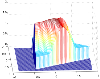
Figure 3: The function $L$ with $\alpha=2.5$, $a=1$ and $b=10$.

We first check assumption (1). We consider only the case $l=2$, being the case $l=3$ similar. Let $x\in\mathbb{T}$ be such that $|x-B_{1}|<|x-B_{2}|$. Then necessarily, $|x-B_{2}|>\lambda\sqrt{3}/2$. With our choice of $b$, we deduce that

$$\min\{b,|x-B_{2}|^{-\alpha}\}=|x-B_{2}|^{-\alpha}<\min\{b,|x-B_{1}|^{-\alpha}\}.$$

By construction

$$c_{2}(x)=\frac{a+\min\{b,|x-B_{1}|^{-\alpha}\}+\min\{b,|x-B_{3}|^{-\alpha}\}}{\min\{b,|x-B_{2}|^{-\alpha}\}},\qquad x\in\mathbb{T},$$

and so (1) follows easily.

It is immediate to check that $c$ is a Lipschitz function, and the axial symmetry around the straight line determined by $0$ and $B_{1}$ maps $B_{2}$ into $B_{3}$. Thus assumptions (1) and (6) follow.

In order to check (1), we note that if $x\in\mathbb{T}_{1}$, then, for $l=2,3$, $|x-B_{l}|\geq|x-B_{1}|$. Thus, for $l=2,3$, $\min\{b,|x-B_{l}|^{-\alpha}\}\leq\min\{b,|x-B_{1}|^{-\alpha}\}$, and we deduce

$$c(x) = \frac{a+\min\{b,|x-B_{2}|^{-\alpha}\}+\min\{b,|x-B_{3}|^{-\alpha}\}}{\min\{b,|x-B_{1}|^{-\alpha}\}}$$

$$\leq \frac{a}{\min\{b,|x-B_{1}|^{-\alpha}\}}+2$$

$$\leq \lambda^{\alpha}a+2=c(0),$$

where the last inequality is strict if $x\neq 0$. Similarly, $a+\min\{b,|x-B_{2}|^{-\alpha}\}+\min\{b,|x-B_{3}|^{-\alpha}\}$ is minimized for $x=B_{1}$ and $\min\{b,|x-B_{1}|^{-\alpha}\}$ is maximized for $x=B_{1}$. So, for $x\neq B_{1}$, $c(x)>c(B_{1})$.

Now we check assumption (5). Define

$$A_{l}=\{x\in\mathbb{T}\dvtx|x-B_{l}|<b^{-1/\alpha}\},\qquad l=1,2,3.$$

With our choice of $b$, if $l\neq m$, we have $A_{l}\cap A_{m}=\varnothing$. Define

$$A_{0}=\mathbb{T}\setminus(A_{1}\cup A_{2}\cup A_{3}).$$

Note that, by construction, on each set $A_{l}$, $l=0,1,2,3$, the sign of $b-|x-B_{m}|^{-\alpha}$ is constant for each $m=1,2,3$. To prove (5), we shall check that, for all $t\geq 0$ and $l=0,1,2,3$,

$$\ell\bigl{(}A_{l}\cap c^{-1}(\{t\})\bigr{)}=0.$$ (66)

We shall only prove the above equality for $l=0$, the other cases can be shown similarly. Note that

$$c(x)=|x-B_{1}|^{\alpha}(a+|x-B_{2}|^{-\alpha}+|x-B_{3}|^{-\alpha})\qquad\forall x\in A_{0}.$$

Using polar coordinates we have

$$\ell\bigl{(}A_{0}\cap c^{-1}(\{t\})\bigr{)}=\int_{0}^{2\pi}d\theta\int_{0}^{\infty}\mathbh{1}\{r{e}^{i\theta}\in A_{0}\}\mathbh{1}\{c(r{e}^{i\theta})=t\}r\,dr.$$

We shall check that, for an arbitrarily fixed $\theta\in[0,2\pi)$, the function

$$c_{\theta}(r)=a|r{e}^{i\theta}-B_{1}|^{\alpha}+\biggl{(}\frac{|r{e}^{i\theta}-B_{1}|}{|r{e}^{i\theta}-B_{2}|}\biggr{)}^{\alpha}+\biggl{(}\frac{|r{e}^{i\theta}-B_{1}|}{|r{e}^{i\theta}-B_{3}|}\biggr{)}^{\alpha},\qquad r\in I_{\theta},$$

is strictly monotone, where

$$I_{\theta}=\{r\dvtx r\geq 0,r{e}^{i\theta}\in\mathbb{T}\}.$$

So, for any fixed $\theta\in[0,2\pi)$, the function $\mathbh{1}\{r{e}^{i\theta}\in A_{0}\}\mathbh{1}\{c(r{e}^{i\theta})=t\}$ is different from $0$ for at most one $r$, and therefore equality (66) for $l=0$ follows. In the following we shall only prove that $c_{\theta}$ is strictly decreasing on $I_{\theta}$ for $\theta\in[-\pi/6,\pi/6]$, the other cases can be treated similarly. First, note that since $\theta\in[-\pi/6,\pi/6]$, as $r$ increases, $|r{e}^{i\theta}-B_{1}|^{\alpha}$ decreases, while $|r{e}^{i\theta}-B_{3}|^{\alpha}$ increases. Thus, $r\mapsto a|r{e}^{i\theta}-B_{1}|^{\alpha}$ and $r\mapsto(\frac{|r{e}^{i\theta}-B_{1}|}{|r{e}^{i\theta}-B_{3}|})^{\alpha}$ are decreasing. Note also that, for $\theta\in[-\pi/6,0]$, as $r$ increases, $|r{e}^{i\theta}-B_{2}|^{\alpha}$ increases. Thus it suffices to prove that, for a fixed $\theta\in(0,\pi/6]$, the function

$$L_{\theta}(r)=\frac{|r{e}^{i\theta}-B_{1}|^{2}}{|r{e}^{i\theta}-B_{2}|^{2}},\qquad r\in\biggl{[}0,\lambda\biggl{(}2\cos\biggl{(}\frac{\pi}{6}-\theta\biggr{)}\biggr{)}^{-1}\biggr{]},$$

is nonincreasing. Consider the orthonormal basis $\{\mathbf{e}_{1},\mathbf{e}_{2}\}$ with $\mathbf{e}_{1}={e}^{i{\pi}/{6}}$ and $\mathbf{e}_{2}={e}^{-i{\pi}/{3}}$. Setting $\beta=\pi/6-\theta\in[0,\pi/6)$, $y_{1}=\lambda/2$ and $y_{2}=\lambda\sqrt{3}/2$, we have

$$r{e}^{i\theta}=r\cos\beta\mathbf{e}_{1}+r\sin\beta\mathbf{e}_{2},\qquad B_{1}=y_{1}\mathbf{e}_{1}+y_{2}\mathbf{e}_{2},\qquad B_{2}=y_{1}\mathbf{e}_{1}-y_{2}\mathbf{e}_{2}$$

and

$$L_{\theta}(r)=\frac{(y_{1}-r\cos\beta)^{2}+(y_{2}-r\sin\beta)^{2}}{(y_{1}-r\cos\beta)^{2}+(y_{2}+r\sin\beta)^{2}}.$$

The derivative $L^{\prime}_{\theta}(r)$ of $L_{\theta}(r)$ has the same sign of

$$-\bigl{(}\cos\beta(y_{1}-r\cos\beta)+\sin\beta(y_{2}-r\sin\beta)\bigr{)}\bigl{(}(y_{1}-r\cos\beta)^{2}+(y_{2}+r\sin\beta)^{2}\bigr{)}$$

$$\qquad{}+\bigl{(}\cos\beta(y_{1}-r\cos\beta)-\sin\beta(y_{2}+r\sin\beta)\bigr{)}$$

$$\qquad\quad{}\times\bigl{(}(y_{1}-r\cos\beta)^{2}+(y_{2}-r\sin\beta)^{2}\bigr{)}.$$

After simplification, we get easily that $L^{\prime}_{\theta}(r)$ has the same sign of

$$-2r\cos\beta\sin\beta-\bigl{(}(y_{1}-r\cos\beta)^{2}+y_{2}^{2}-r^{2}\sin^{2}\beta\bigr{)}\sin\beta.$$

This last expression is less than or equal to $0$. Indeed, for $r\in[0,\lambda(2\cos\beta)^{-1}]$, we have $0\leq r\sin\beta\leq y_{2}$. Hence $L_{\theta}$ is nonincreasing on its domain.

Finally, we check that, for fixed $\alpha>2$ and $a>0$, it is possible to determine $b>(\lambda\sqrt{3}/2)^{-\alpha}$ so that the second inequality in (1) holds. We deduce

$$\quad\int_{\mathbb{T}_{2}}c(x)\,dx \geq \int_{\mathbb{T}_{2}}\frac{a+\sum_{l=2}^{3}\min\{b,|x-B_{l}|^{-\alpha}\}}{(\lambda\sqrt{3}/2)^{-\alpha}}\,dx$$ (67)

$$= \int_{\mathbb{T}_{2}}\frac{a+\min\{b,|x-B_{2}|^{-\alpha}\}+|x-B_{3}|^{-\alpha}}{(\lambda\sqrt{3}/2)^{-\alpha}}\,dx$$

$$\geq \frac{a/3}{(\lambda\sqrt{3}/2)^{-\alpha}}+\frac{\pi b^{1-(2/\alpha)}/6}{(\lambda\sqrt{3}/2)^{-\alpha}}$$

$${}+\bigl{(}\lambda\sqrt{3}/2\bigr{)}^{\alpha}\int_{\mathbb{T}_{2}}|x-B_{3}|^{-\alpha}\,dx.$$

Here (67) and (.6) follow since on $\mathbb{T}_{2}$ we have $|x-B_{l}|^{-\alpha}<(\lambda\sqrt{3}/2)^{-\alpha}<b$ for $l=1,3$; (.6) is consequence of the inequality $|x-B_{2}|^{-\alpha}>b$, for any $x\in A_{2}\cap\mathbb{T}_{2}$. The claim follows noticing that, due to our choice of $\alpha$, $c(0)/3$ is strictly less than the quantity in (.6), for $b$ large enough.

References

- (1) {bbook}[mr] \bauthor\bsnmBillingsley, \bfnmPatrick\binitsP. (\byear1968). \btitleConvergence of Probability Measures. \bpublisherWiley, \baddressNew York. \bidmr=0233396\endbibitem
- (2) {barticle}[mr] \bauthor\bsnmBordenave, \bfnmCharles\binitsC. (\byear2006). \btitleSpatial capacity of multiple-access wireless networks. \bjournalIEEE Trans. Inform. Theory \bvolume52 \bpages4977–4988. \biddoi=10.1109/TIT.2006.883549, mr=2300367 \endbibitem
- (3) {bbook}[vtex] \bauthor\bsnmButtazzo, \bfnmGiuseppe\binitsG., \bauthor\bsnmGiaquinta, \bfnmMariano\binitsM. and \bauthor\bsnmHildebrandt, \bfnmStefan\binitsS. (\byear1998). \btitleOne-Dimensional Variational Problems. \bseriesOxford Lecture Series in Mathematics and Its Applications \bvolume15. \bpublisherOxford Univ. Press, \baddressNew York. \bidmr=1694383 \endbibitem
- (4) {bbook}[mr] \bauthor\bsnmDembo, \bfnmAmir\binitsA. and \bauthor\bsnmZeitouni, \bfnmOfer\binitsO. (\byear1998). \btitleLarge Deviations Techniques and Applications, \bedition2nd ed. \bseriesApplications of Mathematics (New York) \bvolume38. \bpublisherSpringer, \baddressNew York. \bidmr=1619036 \endbibitem
- (5) {bbook}[mr] \bauthor\bsnmDudley, \bfnmR. M.\binitsR. M. (\byear1999). \btitleUniform Central Limit Theorems. \bseriesCambridge Studies in Advanced Mathematics \bvolume63. \bpublisherCambridge Univ. Press, \baddressCambridge. \bidmr=1720712 \endbibitem
- (6) {bbook}[mr] \bauthor\bsnmMurray, \bfnmJ. D.\binitsJ. D. (\byear1984). \btitleAsymptotic Analysis, \bedition2nd ed. \bseriesApplied Mathematical Sciences \bvolume48. \bpublisherSpringer, \baddressNew York. \bidmr=740864 \endbibitem
- (7) {barticle}[mr] \bauthor\bsnmO’Connell, \bfnmNeil\binitsN. (\byear2000). \btitleA large deviations heuristic made precise. \bjournalMath. Proc. Cambridge Philos. Soc. \bvolume128 \bpages561–569. \biddoi=10.1017/S0305004199004260, mr=1744101 \endbibitem
- (8) {bbook}[mr] \bauthor\bsnmRoyden, \bfnmH. L.\binitsH. L. (\byear1988). \btitleReal Analysis, \bedition3rd ed. \bpublisherMacmillan, \baddressNew York. \bidmr=1013117 \endbibitem
- (9) {bbook}[vtex] \bauthor\bsnmTse, \bfnmD.\binitsD. and \bauthor\bsnmViswanath, \bfnmP.\binitsP. (\byear2005). \btitleFundamentals of Wireless Communication. \bpublisherCambridge Univ. Press, \baddressNew York. \endbibitem