Direct photons at forward rapidities in high-energy pp collisions

Abstract

We investigate direct photon production in $pp$ collisions at the energies of RHIC, CDF and LHC, at different rapidities employing various color-dipole models. The cross section peaks at forward rapidities due to the abelian dynamics of photon radiation. This opens new opportunities for measurement of direct photons at forward rapidities, where the background from radiative hadronic decays is strongly suppressed. Our model calculations show that photon production is sensitive to the gluon saturation effects, and strongly depends on the value of the anomalous dimension.

I Introduction

Photons radiated in hadronic collisions not via hadronic decays are usually called direct. They carry important information about the collision dynamics, not disturbed by final state interactions. In particular, the hadronization stage is absent, so the theoretical interpretation is simpler that in the case of hadron production. A unified description for radiation of virtual (Drell-Yan reaction) and real photons within the color dipole approach was proposed in hir ; kst1 . This description does not need to be corrected either for higher order effects (K-factor, large primordial transverse momentum), or for the main higher twist terms. The corresponding phenomenology is based on the universal dipole cross section fitted to DIS data and provides a rather good description of data, both the absolute normalization and the transverse momentum dependence amir0 . Predictions of the inclusive direct photon spectra for the LHC at midrapidity and the azimuthal asymmetry of produced prompt photons in the same framework are given in Refs. us-3 ; asy0 . Comparison with the predictions of other approaches at the LHC can be found in Refs. lhc-hic ; nlhc .

Intensive study of the dynamics of hadronic interactions at high energies and search for signatures of nonlinear QCD effects, like saturation glr , or color glass condensate (CGC) mv , have led to considerable experimental progress towards reaching smallest Bjorken $x$. The typical experimental set up at modern colliders allows to detect particles produced in hard reactions in the central rapidity region, while the most energetic ones produced at forward (backward) rapidities escape detection. The first dedicated measurements of hadron production at forward rapidities, by the BRAHMS experiment in deuteron-gold collisions at RHIC brahms , disclosed an interesting effect of nuclear suppression, which can be interpreted as a breakdown of QCD factorization knpjs . The zero degree calorimeters detecting neutral particles, neutrons and photons, at maximal rapidities are being employed at RHIC and are planned to be installed at LHC. One could increase the transverse momentum coverage of these detectors by moving them away from the beam axis. Through this note we would like to encourage the experimentalists to look up at these opportunities.

The important advantage of measurements of direct photons at forward rapidities is a significant enhancement of the signal-to-background ratio. Indeed, the photons radiated by the electric current of the projectile quarks, which stay in the fragmentation region of the beam, form a bump at forward rapidities (see Fig. 5). At the same time, gluons are radiated via nonabelian mechanisms by the color current which flows across the whole rapidity interval. Therefore gluons are radiated mainly in the central rapidity region gb , and are strongly suppressed in the beam fragmentation region. Such a suppression is even more pronounced for hadrons from gluon fragmentation, and for photons from radiative decays of those hadrons. Another source of background photons, hadrons produced via fragmentation of the valence quarks is also strongly suppressed due to the shift towards small fractional momenta related to the quark fragmentation function and the kinematics of radiative decay. Thus, direct photon production at forward rapidities should be substantially cleared up.

Here we perform calculations for direct photon production at large $p_{T}$ and various rapidities in proton-proton collisions at the energies of RHIC, Tevatron and LHC. We employ the color dipole approach and compare the predictions of several contemporary models for the dipole cross section, based on the idea of gluon saturation.

II Photon radiation in the color dipole formalism

Production of direct photons in the target rest frame should be treated as electromagnetic bremsstrahlung by a quark interacting with the target, as is illustrated in Fig. 1 in the single gluon approximation, which should be accurate at large transverse momenta of the photon. Since the quark trajectories before and after photon radiation have different impact parameters, and the corresponding terms in the bremsstrahlung amplitude have different signs, one arrives at an expression, which is formally identical to the amplitude of an inelastic dipole-target interaction hir . This is only a formal procedure of calculation, while no real dipole is involved in the process of radiation.

Calculation of the transverse momentum distribution is more involved kst1 , since the direct and complex conjugated amplitudes correspond to incoming quarks with different impact parameters. It substantially simplifies after integration over transverse momentum of the recoil quark, so one is left with two dipoles of different sizes $\vec{r}_{1}$ and $\vec{r}_{2}$, and the cross section gets the factorized form kst1 ; amir0 ,

$$\frac{d\sigma(qp\to\gamma X)}{d(ln\alpha)\,d^{2}{\vec{p}_{T}}}(\vec{p}_{T},\alpha)=\frac{1}{(2\pi)^{2}}\sum_{in,f}\int d^{2}{r}_{1}d^{2}{r}_{2}$$ (1)

$$\times e^{i\vec{p}_{T}\cdot(\vec{r}_{1}-\vec{r}_{2})}\phi^{\star}_{\gamma q}(\alpha,\vec{r}_{1})\phi_{\gamma q}(\alpha,\vec{r}_{2})\Sigma_{\gamma}(x_{2},\vec{r}_{1},\vec{r}_{2},\alpha),$$

where $\vec{r}_{1}$ and $\vec{r}_{2}$ are the quark-photon transverse separations in the direct and complex conjugated amplitudes respectively; $\alpha=p_{\gamma}^{+}/p_{q}^{+}$ denotes the fractional light-cone (LC) momentum of the radiated photon. Correspondingly, the transverse displacements of the recoil quarks in the two amplitudes are $\alpha r_{1}$ and $\alpha r_{2}$ respectively. The LC distribution amplitude for the $q\gamma$ Fock component with transverse separation $\vec{r}$ has the form,

$$\phi_{\gamma q}(\alpha,\vec{r}_{T})=\frac{\sqrt{\alpha_{em}}}{2\,\pi}\,\chi_{f}\,\widehat{O}\,\chi_{i}\,K_{0}(m_{q}\alpha r_{T}).$$ (2)

Here $\chi_{i,f}$ are the spinors of the initial and final quarks and $K_{0}(x)$ is the modified Bessel function. The operator $\widehat{O}$ has the form,

$$\widehat{O}=i\,m_{f}\alpha^{2}\,\vec{e^{*}}\cdot(\vec{n}\times\vec{\sigma})\,+\alpha\,\vec{e^{*}}\cdot(\vec{\sigma}\times\vec{\nabla})-i(2-\alpha)\,\vec{e^{*}}\cdot\vec{\nabla}\ ,$$ (3)

where $\vec{e}$ is the polarization vector of the photon; $\vec{n}$ is a unit vector along the projectile momentum; and $\vec{\nabla}$ acts on $\vec{r}_{T}$. The effective quark mass $m_{q}$ serves as infra-red cutoff parameter, which we fix at $m_{q}\approx 0.14\,\mbox{GeV}$, since all dipole parametrizations considered in this paper also assume the light quark mass equal to $0.14$ GeV.

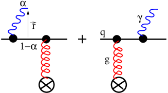
Figure 1: Direct photon radiation by a quark interacting with a gluon in the target.

In equation (1) the effective dipole cross-section $\Sigma_{\gamma}$ is a linear combination of the $\bar{q}q$ dipole-proton cross sections,

$$\Sigma_{\gamma}(x_{2},\vec{r}_{1},\vec{r}_{2},\alpha) = \frac{1}{2}\{\sigma_{q\bar{q}}(x_{2},\alpha r_{1})+\sigma_{q\bar{q}}(x_{2},\alpha r_{2})\}$$ (4)

$$- \frac{1}{2}\sigma_{q\bar{q}}(x_{2},\alpha(\vec{r}_{1}-\vec{r}_{2})).$$

Here and in what follows $x_{1,2}$ are the Bjorken variable of the beam and target partons,

$$x_{1,2}=\frac{p_{T}}{\sqrt{s}}\,e^{\pm\eta},$$ (5)

and $\eta$ is the photon rapidity in the c.m. of $pp$ collision.

Since only quarks and antiquarks can radiate photons, the hadronic cross section is given by the convolution of the partonic cross section Eq. (1) with the proton structure function $F_{2}^{p}$ joerg ; amir0 ; scho ,

$$\frac{d\sigma(pp\to\gamma X)}{dx_{F}d^{2}\,{p}_{T}}=\frac{1}{x_{1}+x_{2}}\int\limits_{x_{1}}^{1}d\alpha\,F_{2}^{p}\left({x_{1}\over\alpha},Q^{2}\right)\,\frac{d\sigma(qp\to\gamma X)}{d\alpha\,d^{2}{p}_{T}},$$ (6)

where $x_{F}=x_{1}-x_{2}$ is the Feynman variable. This relation needs commenting. The transverse momentum distribution of quark bremsstrahlung should be convoluted with the primordial transverse motion of the projectile quark. Differently from the parton model, in the dipole approach one should rely on the quark distribution function taken at a soft scale. Evolution to the hard scale is performed via gluon radiation, which is encoded into the phenomenological dipole cross section fitted to DIS data for the proton structure function. Since the quark primordial motion with a small (soft) mean transverse momentum does not affect the photons radiated with large $p_{T}$ amir0 , we neglect the transverse momentum convolution and use the integrated quark distribution.

However, a word of caution is in order. The dipole cross section $\sigma_{\bar{q}q}(x_{2},r)$ includes gluon radiation which performs the $Q^{2}$ evolution and leads to an increase of the transverse momentum of the projectile quark. However, it misses the $Q^{2}$ evolution of the $x_{1}$-distribution, which is especially important at forward rapidities (see discussion in bgks ), since the quark distribution falls off at $x_{1}\to 1$ much steeper at high $Q^{2}$. In order to account for this effect and provide the correct $x_{1}$-distribution, we take the integrated quark distribution in (6) at the hard scale.

We use the parametrization for the proton structure function given in Ref. ps . Following Ref. amir0 , for the hard scale entering the proton structure function in Eq. (6), we choose $Q=p_{T}$.

III Models for the dipole cross section

The dipole cross-section is theoretically unknown and should be fitted to data. Several parametrizations proposed in the literature are employed here to investigate the uncertainties and differences among various models.

A popular parametrization proposed by Golec-Biernat and Wüsthoff (GBW) model gbw is based on the idea of gluon saturation. This model is able to describe DIS data with the dipole cross-section parametrized as,

$$\sigma_{q\bar{q}}^{\text{GBW}}(x,\vec{r})=\sigma_{0}\left(1-e^{-r^{2}Q_{s}^{2}(x)/4}\right),$$ (7)

where $x$-dependence of the saturation scale is given by $Q_{s}^{2}(x)=(x_{0}/x)^{\lambda}~{}\text{GeV}^{2}$. The parameters $\sigma_{0}=20.1$ mb, $x_{0}=5.16\times 10^{-4}$, and $\lambda=0.289$ were determined from a fit to $F_{2}$ without charm quarks. A salient feature of the model is that for decreasing $x$, the dipole cross section saturates at smaller dipole sizes. The saturation scale in the GBW reduces with the inclusion of the charm quark gbw-nn . After inclusion of the charm quark with mass $m_{c}=1.5$ GeV, the parameters of the GBW model changed to $\sigma_{0}=23.9$ mb, $x_{0}=1.11\times 10^{-4}$ , and $\lambda=0.287$. Both parametrization sets give a good description of DIS data at $x<0.01$ and $Q^{2}\in[0.25,45]$ gbw-nn .

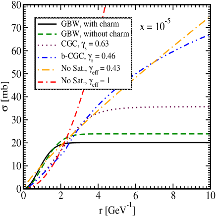
Figure 2: The total dipole-proton cross section $\sigma_{q\bar{q}}(x,r)$ at a fixed $x=10^{-5}$ in various dipole models introduced in Sec. III.

One of the obvious shortcoming of the GBW model is that it does not match the QCD evolution (DGLAP) at large values of $Q^{2}$. This failure can be clearly seen in the energy dependence of $\sigma^{\gamma^{\star}p}_{tot}$ for $Q^{2}>20~{}\text{GeV}^{2}$, where the the model predictions are below the data gbw ; gbw-d .

A modification of the GWB dipole parametrization model, Eq. (7), was proposed in Ref. gbw-d by Bartels, Golec-Biernat and Kowalski (GBW-DGLAP)

$$\sigma_{q\bar{q}}^{\text{GBW-DGLAP}}(x,\vec{r})=\sigma_{0}\left(1-exp\left(-\frac{\pi^{2}r^{2}\alpha_{s}(\mu^{2})xg(x,\mu^{2})}{3\sigma_{0}}\right)\right),$$ (8)

where the scale $\mu^{2}$ is related to the dipole size by

$$\mu^{2}=\frac{C}{r^{2}}+\mu_{0}^{2}.$$ (9)

Here the gluon density $g(x,\mu^{2})$ is evolved to the scale $\mu^{2}$ with the leading order (LO) DGLAP equation. Moreover, the quark contribution to the gluon density is neglected in the small $x$ limit. The initial gluon density is taken at the scale $Q_{0}^{2}=1\text{GeV}^{2}$ in the form

$$xg(x,\mu^{2})=A_{g}x^{-\lambda_{g}}(1-x)^{5.6},$$ (10)

where the parameters $C=0.26$, $\sigma_{0}=23~{}\text{mb},\mu_{0}^{2}=0.52~{}\text{GeV}^{2}$, $A_{g}=1.20$ and $\lambda_{g}=0.28$ are fixed from a fit to the DIS data for $x<0.01$ and in a range of $Q^{2}\in[0.1,500]$ $\text{GeV}^{2}$ gbw-d . The dipole size determines the evolution scale $\mu^{2}$ through Eq. (9). The evolution of the gluon density is performed numerically for every dipole size $r$ during the integration of Eq. (1). Therefore, the DGLAP equation is now coupled to our master equation (1). It is important to stress that the GBW-DGLAP model preserves the successes of the GBW model at low $Q^{2}$ and its saturation property for large dipole sizes, while incorporating evolution of the gluon density by modifying the small-$r$ behaviour of the dipole size.

Since the linear DGLAP evolution may not be appropriate for the saturation regime, Iancu, Itakura and Munier proposed an alternative color glass condensate (CGC) model CGC0 , based on the Balitsky-Kovchegov (BK) equation bk . The dipole cross section is parametrized as,

$$\sigma_{q\bar{q}}^{\text{CGC}}(x,r)=\sigma_{0}\begin{cases}\mathcal{N}_{0}\left(\frac{rQ_{s}}{2}\right)^{2\left(\gamma_{s}+\frac{1}{\kappa\lambda Y}\ln\frac{2}{rQ_{s}}\right)}&:\quad rQ_{s}\leq 2\\ 1-\mathrm{e}^{-A\ln^{2}(BrQ_{s})}&:\quad rQ_{s}>2\end{cases},$$ (11)

where $Q_{s}\equiv Q_{s}(x)=(x_{0}/x)^{\lambda/2}$ GeV, $Y=\ln(1/x)$, and $\kappa=\chi^{\prime\prime}(\gamma_{s})/\chi^{\prime}(\gamma_{s})$ where $\chi$ is the LO BFKL characteristic function. The coefficients $A$ and $B$ in the second line of (11) are determined uniquely from the condition that $\sigma(x,r)$, and its derivative with respect to $rQ_{s}$, are continuous at $rQ_{s}=2$:

$$A=-\frac{\mathcal{N}_{0}^{2}\gamma_{s}^{2}}{(1-\mathcal{N}_{0})^{2}\ln(1-\mathcal{N}_{0})},\qquad B=\frac{1}{2}\left(1-\mathcal{N}_{0}\right)^{-\frac{(1-\mathcal{N}_{0})}{\mathcal{N}_{0}\gamma_{s}}}.$$ (12)

The parameters $\gamma_{s}=0.63$ and $\kappa=9.9$ are fixed at the LO BFKL values. The others parameters $\mathcal{N}_{0}=0.7$, $\sigma_{0}=35.7$ mb, $x_{0}=2.7\times 10^{-7}$ and $\lambda=0.177$ were fitted to $F_{2}$ for $x<0.01$ and $Q^{2}<45$ $\text{GeV}^{2}$ and including a charm quark with $m_{c}=1.4$ GeV. Notice that for small $rQ_{s}\leq 2$, the effective anomalous dimension $1-\gamma_{s}$ in the exponent in the upper line of Eq. (11) rises from the LO BFKL value towards the DGLAP value.

It should be stressed that this CGC model is built based on the solution of Ref. LT for $r\,Q_{s}\,>2\,$ and a form of the solution for $rQ_{s}\leq 1$, but in the vicinity of $r\propto 1/Q_{s}$ it is given in Refs. IIM ; MUT .

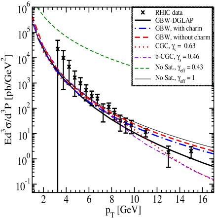
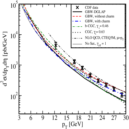
Figure 3: Inclusive direct photon spectra calculated with various color-dipole models at mid-rapidity $\eta=0$ at the energies of RHIC, $\sqrt{s}=200$ GeV (upper panel), and Tevatron, $\sqrt{s}=1.8$ TeV (lower panel). The NLO QCD curve is from the authors of reference ppqcd (given in table 3 of Ref. cdf1 ). Experimental data are from the PHENIX experiment rhic at $\eta=0$, and from the CDF experiment cdf1 ; cdf at $|\eta|<0.9$. The error bars are the linear sum of the statistical and systematic uncertainties.

Notice that calculation of the $p_{T}$-distribution given by Eq. (1) needs only knowledge of the total dipole cross section and is independent of the impact parameter dependence of the partial elastic dipole-proton amplitude. Nevertheless, we consider also the model proposed by Watt and Kowalski bccc . Although the main focus of this model is the impact parameter dependence (b-CGC), which is irrelevant for our calculations, the integrated cross section is different from the above mentioned models,

$$\sigma_{q\bar{q}}^{\text{b-CGC}}(x,r)=2\int d^{2}b\,\sigma_{q\bar{q}}^{\text{CGC}}(x,r,b)\,,$$ (13)

where $\sigma_{q\bar{q}}^{\text{CGC}}(x,r,b)$ is given by Eq. (11) with the saturation scale $Q_{s}$ which now depends on impact parameter,

$$Q_{s}\equiv Q_{s}(x,b)=\left(\frac{x_{0}}{x}\right)^{\frac{\lambda}{2}}\;\left[\exp\left(-\frac{b^{2}}{2B_{\rm CGC}}\right)\right]^{\frac{1}{2\gamma_{s}}}.$$ (14)

The parameter $B_{\rm CG}=7.5\text{GeV}^{-2}$ is fitted to the $t$-dependence of exclusive $J/\Psi$ photoproduction. It has been shown that if one allows the parameter $\gamma_{s}$ to vary along side with other parameters (in contrast with CGC fitting procedure where $\gamma_{s}$ is fixed with LO BFKL value), it results in a significantly better description of data for $F_{2}$ with the value of $\gamma_{s}=0.46$, which is remarkably close to the value of $\gamma_{s}=0.44$ recently obtained from the BK equation bkk . Other parameters obtained from the fit are: $\mathcal{N}_{0}=0.558$, $x_{0}=1.84\times 10^{-6}$ and $\lambda=0.119$.

In order to demonstrate the importance of saturation, we will also use a non-saturated model (No Sat) fitted to $F_{2}$ with $x\leq 0.01$ and $Q^{2}\in[0.25,45]~{}\text{GeV}^{2}$:

$$\frac{d\sigma_{q\bar{q}}^{\text{No Sat}}}{d^{2}\vec{b}}=2\mathcal{N}_{0}\left(\frac{rQ_{s}}{2}\right)^{2\gamma_{eff}}$$ (15)

where $Q_{s}$ is defined in Eq. (14). The parameter $\gamma_{eff}$ is defined for $rQ_{s}\leq 2$ as $\gamma_{eff}=\gamma_{s}+\frac{1}{\kappa\lambda Y}\ln\frac{2}{rQ_{s}}$, and for $rQ_{s}>2$ as $\gamma_{eff}=\gamma_{s}$. The other parameters are given by $\gamma_{s}=0.43$, $\mathcal{N}_{0}=0.568$, $x_{0}=1.34\times 10^{-6}$ and $\lambda=0.109$ bccc . Surprisingly, the fit obtained with such an oversimplified model is as good as the other models with $\chi^{2}/\text{d.o.f.}=0.92$ (although it should certainly fail to explain data on diffractive DIS kps , which are sensitive mainly to large size dipoles). Notice that we use here the No Sat model for a qualitative argumentation.

At first sight this result could be used as an argument that the data is not sensitive to the saturation effect. However, the actual meaning of this exercise is quite opposite. It is well known that the saturation effects start being essential when the anomalous dimension reaches the value $\gamma_{cr}=1-\gamma_{eff}=0.37$ (see Refs. glr ; GAMMA ; MUT ). We will show that at very forward rapidities at LHC, the diffusion term in the anomalous dimension is less important. Therefore, what we actually demonstrate is that the value of the anomalous dimension should be larger than $\gamma_{cr}$ at very forward rapidities for LHC, and because of this the saturation effects have to be taken into account.

The second comment on this model (see Ref. bccc ) is that it is actually a model which contains saturation, and the difference with the CGC model (see Eq. (11)) is only one: this model is written for dipoles with sizes close to $1/Q_{s}$. Indeed, comparing Eq. (11) and Eq. (15) one can see that they treat differently the region $r\,Q_{s}\,>\,1$. The CGC model describes this region as solution to the BK equation deeply in the saturation region LT , with a phenomenological matching at $r\,Q_{s}=2$, while this model uses the solution to the BK equation MUT ; IIM ; LT for $r\,Q_{s}>\,2$ but $r$ close to $1/Q_{s}$. Therefore, it is not appropriate to call this model “no saturation model”, nevertheless, we use this name as a terminology.

Summarizing, we can claim that direct photon production is sensitive to saturation effects. In conclusion, the success of the so-called ‘no saturation model’ can be interpreted such that at the LHC we will be still sensitive to the kinematic region close to the saturation scale.

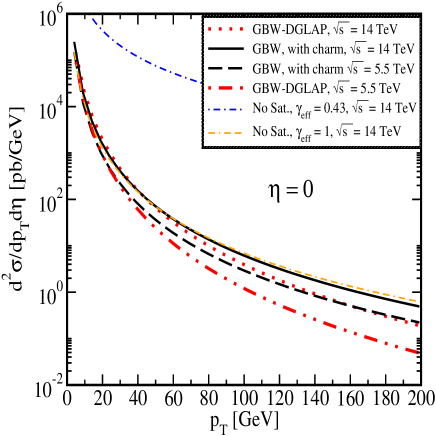
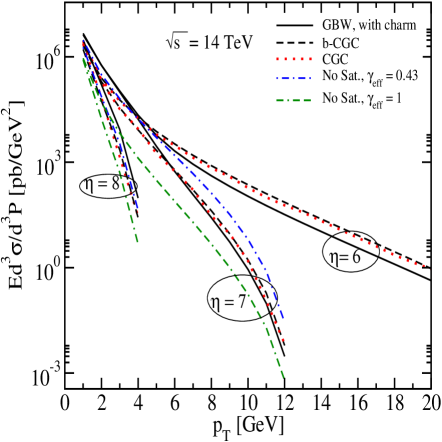
Figure 4: Direct photon spectra obtained from various dipole model at midrapidity (upper panel) and forward rapidities (lower panel) at the LHC energies for $pp$ collisions.

IV Numerical results and discussion

In Fig. 3, we compare predictions of various dipole models with data for inclusive prompt-photon production from RHIC at $\sqrt{s}=200$ GeV and from the Tevatron at $\sqrt{s}=1.8$ TeV. A word of caution is in order here. All the above parametrizations for the dipole cross-section have been fitted to DIS data at $x\leq 0.01$. This corresponds to $p_{T}\leq 2$ GeV at the RHIC energy , so the PHENIX data plotted in the upper panel of Fig. 3 are not suited for a model test. Notice that the CDF data plotted in the bottom panel of Fig. 3 were obtained with a so called isolation cut, which is aimed at suppression of the overwhelming background of secondary photons originated from radiative hadron decays. This might change the cross-section within $10-20\%$ for the CDF kinematics cdf .

One can see from Fig. 3 that various dipole models presented in the previous section with explicit saturation give rather similar results at small $p_{T}$. At high $p_{T}$, CGC, b-CGC and GBW-DGLAP models which incorporate QCD evolution provides a better description of data compared to the GBW model. The No Sat model with the diffusion term, defined in Eq. (15), gives similar results as the b-CGC model for both RHIC and CDF energies (not shown in the plot). In order to understand the role of the diffusion term in the the anomalous dimension, we show in Fig. 3, the results with two extreme limits $\gamma_{eff}=0.43,1$. It is clear that the dipole model without explicit saturation as given by Eq. (15) with $\gamma_{eff}=0.43$, does not describe the data either from PHENIX, or from CDF (we do not show in Fig. 3, No Sat. with $\gamma_{eff}=0.43$ curve for CDF, since it is about two orders of magnitude above the other models and data). However, changing the anomalous dimension to the DGLAP value with $\gamma_{eff}=1$, dramatically changes the results and brings the curves (No Sat model) at both energies of RHIC and Tevatron (at $\eta=0$) within the ranges of other dipole models with saturation and the No Sat model in the presence of the diffusion term. Therefore, the diffusion term in the anomalous dimension is very important at both RHIC and CDF energies.

We have recently shown that the color dipole formulation coupled to the DGLAP evolution provides a better description of data at large transverse momentum compared to the GBW dipole model amir0 . In Fig. 4, upper panel, we show the predictions of the GBW (with charm quark) and the GBW-DGLAP models for LHC energies $\sqrt{s}=5.5,14$ GeV at midrapidity for the transverse momentum up to $p_{T}=200$ GeV. In Fig. 4, lower panel, we show the predictions of various color-dipole models for $\sqrt{s}=14$ GeV at different rapidities. Generally, the discrepancy among predictions of various models at moderate $p_{T}$ is not very large. This can be also seen from Fig. 5 where we compare, as an example, the GBW and b-CGC models, which expose very different structures (see Eqs. (7,13) and Fig. (2)). In the inserted plot in Fig. 4, we show the effect of unitarization within the GBW model, namely using the exponent in Eq. (7) as a dipole cross-section ($r2$ model). One can also see that the discrepancy between the GBW and the $r2$ model increases at forward rapidities, though it is still not appreciable.

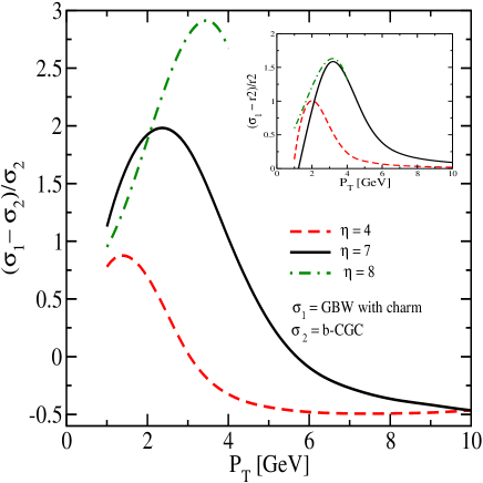
Figure 5: The difference between the GBW and the b-CGC models for the LHC energy $\sqrt{s}=14$ TeV at different rapidities. Inserted plot: the discrepancy between the GBW and the $r2$ model (the GBW model without explicit saturation) at various rapidities for $\sqrt{s}=14$ TeV in $pp$ collisions.

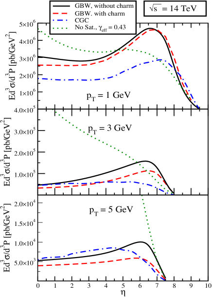
Figure 6: Invariant cross-section for direct photon production in $pp$ collisions as a function of rapidity calculated with various color dipole models $\eta$ for various fixed $p_{T}$ shown in the plots.

In Fig. 4, we also show the results for the model without saturation. At the midrapidity again the results of the No Sat model with the DGLAP anomalous dimension $1-\gamma_{eff}=0$ is close to other saturated models. At the same time, at very forward rapidities, the anomalous dimension $1-\gamma_{eff}=0.57$ which is close to the value predicted from the BK equation bkk , will be in favour of other models. At forward rapidities, the diffusion term in the anomalous dimension is not important more, since it gives similar result as with a fixed $\gamma_{eff}=0.43$. This indicates that direct photons production at different rapidities at LHC is rather sensitive to the saturation. Again, since the values of anomalous dimension turn out to be larger than $\gamma_{cr}=0.37$, such a description of the experimental data indicates at a large saturation effect.

In Fig. 6, the differential cross-section of photon radiation at the energy of LHC is plotted versus rapidity at fixed transverse momenta $p_{T}=1,3,5$ GeV. Calculations were performed with several models for the dipole cross section. All of them lead to a substantial enhancement of the photon production rate at forward rapidities. One can see that the larger the saturation scale is, the stronger is the peak. From Fig. 6, it is again obvious that No Sat model at very forward rapidity is within the dipole model‘s predictions with an explicit saturation. However, the peak disappeared since at about mid-rapidity $\gamma_{eff}=0.43$ is too small. In principle, the peak can be also reproduced in the No Sat model if one allows an anomalous dimension running with energy and transverse momentum $p_{T}$. The appearance of the peak at forward rapidity is a direct consequence of the abelian nature of the electromagnetic interaction. In the case of gluon radiation, the peaks at forward-backward rapidities is be replaced with a kind of plateau at central rapidities, which is indeed observed in data for hadron production.

To conclude, by this letter we encourage measurements of direct photons at forward rapidities in $pp$ collisions at modern colliders . These experiments will be a sensitive tool for search for saturation effects, since they will allow to access the smallest possible values of Bjorken $x$ in the target. Besides, the background of photons from radiative hadronic decays should be significantly suppressed. As we demonstrate in Fig. 6, direct photons are enhanced, even form a bump, at forward rapidities. At the same time, gluon nonabelian radiation is known to be strongly suppressed in this region, so hadron and decay photons are also suppressed. We provided predictions for the cross section of direct photon production at various rapidities for $pp$ collisions at LHC employing different models for the dipole-proton total cross section.

- (1) B.Z. Kopeliovich, Soft Component of Hard Reactions and Nuclear Shadowing (DIS, Drell-Yan reaction, heavy quark production), in proc. of the Workshop Hirschegg’95: Dynamical Properties of Hadrons in Nuclear Matter, Hirschegg, January 16-21,1995, ed. by H. Feldmeier and W. Nörenberg, Darmstadt, 1995, p. 102 ( hep-ph/9609385).
- (2) B.Z. Kopeliovich, A. Schäfer and A. V. Tarasov, Phys. Rev. C59 (1999) 1609.
- (3) B. Z. Kopeliovich, E. M. Levin and I. Schmidt, work in progress.
- (4) B. Z. Kopeliovich, A. H. Rezaeian, H. J. Pirner and I. Schmidt, Phys. Lett. B653, 210 (2007)[arXiv:0704.0642].
- (5) A. H. Rezaeian, B. Z. Kopeliovich, H. J. Pirner and I. Schmidt, arXiv:0707.2040.
- (6) B. Z. Kopeliovich, H. J. Pirner, A. H. Rezaeian and I. Schmidt, Phys. Rev. D77, 034011 (2008)[arXiv:0711.3010] ; B. Z. Kopeliovich, A. H. Rezaeian and I. Schmidt, Nucl. Phys. A807, 61 (2008)[arXiv:0712.2829]; B. Z. Kopeliovich, A. H. Rezaeian and I. Schmidt, arXiv:0804.2283.
- (7) N. Armesto et al., J. Phys. G35, 054001 (2008) [arXiv:0711.0974].
- (8) R. E. Blair, S. Chekanov, G. Heinrich, A. Lipatov, and N. Zotov, Proceedings of the HERA-LHC workshop (CERN-DESY), 2007-2008, arXiv:0809.0846.
- (9) L. V. Gribov, E. M. Levin and M. G. Ryskin, Phys. Rept. 100, 1 (1983).
- (10) L. McLerran and R. Venugopalan, Phys. Rev. D49, 2233 (1994); D49, 3352 (1994).
- (11) I. Arsene et al. [BRAHMS Collaboration], Phys. Rev. Lett. 93, 242303 (2004) [arXiv:nucl-ex/0403005].
- (12) B. Z. Kopeliovich, J. Nemchik, I. K. Potashnikova, M. B. Johnson and I. Schmidt, Phys. Rev. C72, 054606 (2005) [arXiv:hep-ph/0501260].
- (13) J. F. Gunion and G. Bertsch, Phys. Rev. D25, 746 (1982).
- (14) B. Z. Kopeliovich, J. Raufeisen and A. V. Tarasov, Phys. Lett. B503, 91 (2001) [arXiv:hep-ph/0012035].
- (15) B. Z. Kopeliovich, A. H. Rezaeian, arXiv:0811.2024.
- (16) S. J. Brodsky, A. S. Goldhaber, B. Z. Kopeliovich and I. Schmidt, Nucl. Phys. B807, 334 (2009) [arXiv:0707.4658].
- (17) SMC Collaboration, Phys. Rev. D58, 112001 (1998).
- (18) K. Golec-Biernat and M. Wüsthoff, Phys. Rev. D59, 014017 (1999); D60, 114023 (1999).
- (19) H. Kowalski, L. Motyka and G. Watt, Phys. Rev. D74, 074016 (2006).
- (20) J. Bartels, K. Golec-Biernat and H. Kowalski, Phys. Rev. D66, 014001 (2002).
- (21) E. Iancu, K. Itakura and S. Munier, Phys. Lett. B590, 199 (2004).
- (22) I. Balitsky, Nucl. Phys. B463, 99 (1996); Y. V. Kovchegov, Phys. Rev. D60, 034008 (1999); Phys. Rev. D61, 074018 (2000).
- (23) E. Levin and K. Tuchin, Nucl. Phys. B573, 833 (2000) [arXiv:hep-ph/9908317]; Nucl. Phys. A691, 779 (2001)[arXiv:hep-ph/0012167].
- (24) E. Iancu, K. Itakura and L. McLerran, Nucl. Phys. A708, 327 (2002)[arXiv:hep-ph/0203137].
- (25) A. H. Mueller and D. N. Triantafyllopoulos, Nucl. Phys. B640, 331 (2002)[arXiv:hep-ph/0205167].
- (26) G. Watt and H. Kowalski, Phys. Rev. D78, 014016 (2008).
- (27) D. Boer, A. Utermann and E. Wessels, Phys. Rev. D75, 094022 (2007)[arXiv:hep-ph/0701219].
- (28) B. Z. Kopeliovich, I. K. Potashnikova and I. Schmidt, Phys. Rev. C73, 034901 (2006) [arXiv:hep-ph/0508277].
- (29) J. Bartels and E. Levin, Nucl. Phys. B387, 617 (1992); S. Munier and R. B. Peschanski, Phys. Rev. D69, 034008 (2004)[arXiv:hep-ph/0310357]; Phys. Rev. Lett. 91, 232001 (2003)[arXiv:hep-ph/0309177].
- (30) M. Gluck, L. E. Gordon, E. Reya and W. Vogelsang, Phys. Rev. Lett. 73, 388 (1994).
- (31) CDF Collaboration, Phys. Rev. D70, 074008 (2004).
- (32) PHENIX Collaboration, Phys. Rev .Lett. 98, 012002 (2007).
- (33) CDF Collaboration, Phys. Rev. Lett. 73, 2662 (1994); 74,1891 (1995).