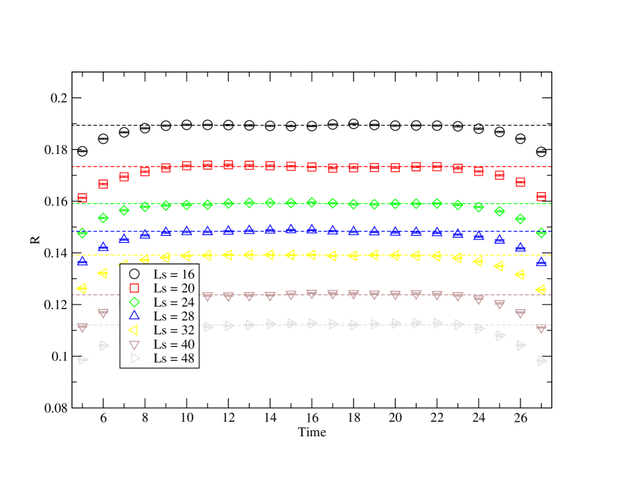
Dynamical simulation of supersymmetric Yang-Mills theory with domain wall fermions
Abstract
We present results from a numerical study of supersymmetric Yang-Mills theory using domain wall fermions. In this particular lattice formulation of the theory, supersymmetry is expected to emerge accidentally in the continuum and chiral limits without any fine-tuning of operators. Dynamical simulations were performed for the gauge group on and lattice space-time volumes and at three different values of the coupling: , and . Results from this study include measurements of the static potential, residual mass, and a chirally extrapolated value for the gluino condensate at . In addition to these, we study the low lying eigenvalues and eigenvectors of the five dimensional Hermitian domain-wall fermion Dirac operator and present evidence that, for the choice of parameters under investigation, features of the spectrum appear qualitatively consistent with strong coupling and the presence of a large residual mass. From the five dimensional eigenvalues we explore the possibility of using the Banks-Casher relation to determine an independent value for the gluino condensate in the chiral limit.
pacs:
11.15.Ha, 11.30.PbI Introduction
In recent years, substantial effort has been devoted toward formulating supersymmetric (SUSY) gauge theories on the lattice.111For recent reviews, see e.g., Feo (2003); Giedt (2006). These efforts have been partially motivated by the fascinating theoretical and technical difficulties associated with the problem, as well as the obvious potential role of SUSY in beyond the standard model physics. Of crucial importance pertaining to the latter point is an understanding of a variety of nonperturbative phenomena, including–but not limited to–dynamical SUSY breaking. An understanding of nonperturbative aspects such as these may in principle be achieved with numerical simulations, provided an appropriate lattice discretization of the theory may be found.
Since naíve lattice discretizations typically break SUSY explicitly, simulations of such theories will generally require a substantial degree of fine-tuning in order to cancel any undesirable SUSY breaking operators which may arise through radiative corrections. Such a task is exceedingly difficult, even when the number of parameters which require fine-tuning are relatively small. However, it has been realized for some time that one of the simplest SUSY theories, supersymmetric Yang-Mills (SYM), may be simulated using conventional lattice discretizations and yet require only a minimal degree of fine-tuning.
The field content of SYM consists of a vector field and a single Majorana fermion which transforms as an adjoint under the gauge group, which for our purposes will be taken to be . The theory possesses an anomalous axial symmetry, however, a discrete subgroup of survives at the quantum level. It is believed that SYM shares a variety of features in common with Quantum Chromodynamics (QCD), such as confinement and chiral symmetry breaking Witten (1997). But in contrast to QCD, SYM is believed to possess discrete chiral symmetry breaking from which results in the possible formation of domain walls but no Goldstone bosons. Although this theory does not possess dynamical SUSY breaking, as implied by a nonvanishing Witten index Witten (1982), it is still believed to exhibit a variety of other features which may be of interest to explore nonperturbatively. Of perhaps greatest interest is whether or not a gluino condensate forms, the spectrum of the theory, and the relationship between the domain wall tension and the gluino condensate.
The low energy spectrum of SYM is believed to consist of massive supermultiplets which may involve glue-glue, glue-gluino as well as gluino-gluino bound states. Although the states within a given supermultiplet are degenerate, at finite gluino mass one expects mass splittings which may be calculated using a variety of effective theories Veneziano and Yankielowicz (1982); Farrar et al. (1998). Lattice simulations of SYM may be used to directly test the predictions of these effective theories, as well as to determine the effects of soft SUSY breaking on observables other than the spectrum.
SYM theory provides an ideal starting point for studying aspects of SUSY numerically while still allowing one to utilize familiar and well understood fermion discretizations. Because the field content of this theory consists only of a vector field and Majorana fermion (and in particular no scalar fields), with conventional lattice discretizations of this theory, the only relevant SUSY violating operator which may arise radiatively is a gluino mass term. In the chiral and continuum limits, SUSY is therefore expected to emerge accidentally at infinite volume. For fermion discretizations that explicitly break chiral symmetry, taking the chiral limit requires tuning the input mass parameter to some critical value, such that the bare mass vanishes.
With the use of a Ginsparg-Wilson Ginsparg and Wilson (1982) fermion discretization such as overlap fermions Neuberger (1998), fine-tuning of the gluino mass term may be entirely avoided. This study utilizes the closely related domain wall fermion (DWF) formalism Kaplan (1992); Narayanan and Neuberger (1993); Shamir (1993), which realizes chiral symmetry in the limit of infinite fifth dimension extent and vanishing input gluino mass. In a typical DWF simulation where the fifth dimension is finite, however, the action receives residual chiral symmetry violating radiative corrections, including an additive mass renormalization. The important advantage that DWF fermions have over other discretizations (which lack chiral symmetry) is that these renormalizations may be removed by taking a controlled and unambiguously determined limit.
In the past, a variety of numerical studies have employed Wilson fermions in order to simulate SYM Montvay (1996); Donini and Guagnelli (1996); Koutsoumbas and Montvay (1997); Montvay (1997); Donini et al. (1998); Koutsoumbas et al. (1998); Montvay (1998); Kirchner et al. (1999); Campos et al. (1999); Montvay (2000); Feo et al. (2000a, b); Farchioni et al. (2002); Montvay (2002); Peetz et al. (2003); Farchioni et al. (2004); Farchioni and Peetz (2005); Demmouche et al. (2008). This discretization requires fine-tuning and formally possesses a sign problem, since the Pfaffian obtained from “integrating out” the fermion degrees of freedom is generally not positive definite.222While one may prove that the fermion Pfaffian for this theory is positive definite in the continuum, positivity is not necessarily guaranteed on the lattice. Studies, however, have found that the Pfaffian phase becomes innocuous in the parameter regime of physical interest and may be effectively handled by phase reweighting techniques. It was observed in Kaplan and Schmaltz (2000) that DWFs have an additional advantage over Wilson fermions in that the fermion Pfaffian is positive definite. With the use of DWFs, one may therefore avoid the task of phase reweighting altogether.
The first and until recently the only study to use DWFs to investigate SYM focused on the chiral limit of the gluino condensate Fleming et al. (2001) at a single lattice spacing. This study was performed by using an inexact, hybrid molecular dynamics R (HMDR) algorithm Gottlieb et al. (1987) which, for the theory under consideration, is prone to finite integration step size errors. Our study offers an improvement over Fleming et al. (2001), by utilizing the rational hybrid Monte Carlo (RHMC) algorithm Clark and Kennedy (2004); Clark et al. (2005, 2006), which is an exact algorithm. Furthermore, due to algorithmic improvements and faster computers, we are able to explore the theory on larger lattices and smaller couplings as well. Recently an independent study of SYM using DWFs was reported by Giedt, et al. in Giedt et al. (2008, 2009).
The primary purpose of our study is to establish a set of sensible simulation parameters, perform basic measurements and provide the necessary ground work for more detailed studies of the theory in the future. As such, we expand the work of Fleming et al. (2001) in several important respects: we 1) establish the lattice scale by measuring the static potential and provide evidence for confinement which is consistent with expectations, 2) determine the size of the residual mass in order to ascertain the proximity to the SUSY point, 3) extrapolate the chiral condensate to the chiral limit using a recent, theoretically motivated fit formula for its dependence and which differs from the formula used in Fleming et al. (2001), 4) study the structure of the low lying eigenvectors and eigenvalues of the Hermitian DWF Dirac operator and attempt to extract an independent value for the chiral condensate using the Banks-Casher relation Banks and Casher (1980). With exception to the third and final points, questions such as these could not be easily addressed in Fleming et al. (2001) due to the limited space-time volumes employed.
Portions of this work have been reported at Lattice 2008 Endres (2008), including results obtained for points 1-3. In this paper we go into greater detail on the analysis of these results, and expand this analysis by including the eigenvalue and eigenvector studies outlined in point 4. We organize this paper as follows. In Sec. II we describe the details of our numerical simulations, including a brief review of the domain wall fermion formalism and conventions, the RHMC algorithm, ensembles and measurement methods. Sec. III is devoted to issues concerning thermalization and autocorrelations, while Sec. IV pertains to measurement details, data analysis and results. In Sec. V, we summarize our findings. Finally, in Appendix A we review some basic properties of Marjorana fermions, which may be less familiar to those readers who specialize in lattice QCD, and specifically derive expressions for some of the gluino-dependent observables studied in this paper.
II Simulation details
II.1 Lattice action and conventions
Dynamical numerical simulations of SYM were performed using a Wilson gauge action and domain wall fermions. The full form of the partition function in Euclidean space-time is given by:
| (1) |
where represents the gauge action and represents the action for domain wall fermions. represents the action for the Pauli-Villars (PV) fields which are required in order to cancel off the UV contributions associated with the bulk fermions in the fifth dimension. Simulations are performed on a lattice, where represents the lattice space-time volume of the four physical dimensions with spatial extent and temporal extent , and represents the size of the unphysical fifth dimension.
The Wilson gauge action is given by:
| (2) |
where represents a plaquette and are link variables which belong to fundamental representation of and are associated with the four dimensional space-time coordinate () and orientation (). As is usual with the domain wall fermion discretization, the gauge field is taken to be independent of the fifth dimension coordinate (). The bare coupling is given by .
The five dimensional DWF Dirac operator is defined by:
| (3) |
where
| (4) |
| (8) |
and the spin projectors 333 in the notation of, for example, reference Furman and Shamir (1995). and are given by:
| (9) |
The gamma matrices in Euclidean space are taken to be Hermitian and satisfy the properties: and (no sum on ); the four dimensional chirality operator is given by . The real link variables belong to the adjoint representation of the gauge group. These may be expressed in terms of fundamental representation link variables which appear in the gauge action via the identity:
| (10) |
where are generators of the fundamental representation of the gauge group which satisfy , with . Finally, and appearing in Eq. 3 represent the domain wall height and input gluino mass, respectively.
The DWF Dirac operator satisfies the following properties:
| (11) | |||||
| (12) |
where , is the reflection operator about the mid-plane in the fifth direction, is the DWF charge conjugation operator and is the standard four dimensional charge conjugation operator which satisfies the usual relations:
| (13) | |||||
| (14) | |||||
| (15) | |||||
| (16) | |||||
| (17) |
Here, are the generators of the adjoint representation of the gauge group which satisfy . The DWF and PV actions are given by:
| (18) |
where we have imposed the DWF and PV Majorana conditions: and . Note that the PV action used in these simulations is not the one introduced in Furman and Shamir (1995) but rather a variant of that action Vranas (1998).
All gluino dependent observables in this study are expressed in terms of the four dimensional gluino interpolating fields , which are defined at the boundaries of the fifth dimension. In terms of the five dimensional fields , the gluino interpolating fields are given by:
| (19) | |||||
| (20) |
For convenience, we also define here the four-dimensional gluino fields which may be associated with the mid-plane in the fifth dimension:
| (21) | |||||
| (22) |
Note that each of the interpolating fields in Eq. 20 and Eq. 22 satisfy the appropriate four dimensional Majorana conditions: and .
Following Furman and Shamir (1995) we may define four-dimensional vector and axial currents and by:
| (23) | |||||
| (24) |
where are the first four components of the five dimensional conserved current, given by:
| (25) |
and the last component is given by:
| (28) |
The divergence of the four dimensional vector and axial currents satisfy
| (29) | |||||
| (30) |
where is the forward finite difference operator and
| (31) | |||||
| (32) |
are the pseudo-scalar densities defined on the walls and midpoint of the fifth dimension, respectively. The axial Takahashi-Ward identity (ATWI) is given by:
| (33) |
where it may be verified that the term involving the midpoint pseudo-scalar density gives rise to the desired axial anomaly Shamir (1994).
II.2 Simulation method
In order to simulate the partition function given by Eq. 1, it is necessary to first integrate out the DWF and PV degrees of freedom. After performing this integration, we are left with an effective action which depends only on the gauge fields and is given by:
| (34) |
where, using the relation , the Pfaffian may be expressed as
| (35) |
Numerical simulations of SYM requires a positive definite fermion Pfaffian in order to unambiguously define the Pfaffian as the square root of a determinant. It may be shown that for domain wall fermions, this is indeed the case and demonstrates an advantage of using this formalism over other discretizations, such as Wilson fermions Kaplan and Schmaltz (2000). By exploiting -Hermiticity described by Eq. 12, we may rewrite the effective action as
| (36) |
where . For the purpose of numerical simulation, we introduce a single complex pseudo-fermion field in order to reproduce the effects of the ratio of fermion determinants given by Eq. 36.444The simultaneous treatment of normal and PV fermion contributions with a single pseudo-fermion field was an idea of M. Clark, and was first introduced in Allton et al. (2007). The resulting partition function is given by:
| (37) |
where the pseudo-fermion action is given by:
| (38) |
Dynamical numerical simulations of Eq. 37 with were performed using a modified version of the Columbia Physics System (CPS)–a software system which is developed and maintained by the RBC collaboration for the purpose of studying lattice Quantum Chromodynamics. Modifications to the software were specifically made in order to accommodate the adjoint character of the fermions being simulated as well as to reduce the gauge group under consideration from down to . We perform numerical simulations of the partition function given by Eq. 37 via the exact rational hybrid Monte Carlo (RHMC) algorithm Clark and Kennedy (2004); Clark et al. (2005, 2006). Details of the parameters used in the approximation of and , for the appropriate rational powers and (i.e., and for the pseudo-fermion refreshment step, and and for the evolution) used in this simulation, may be found in Table 1 and Table 2. Parameters attributed to the PV fields in this study are labeled with the superscript PV. The parameters () and () specify the lower and upper bounds on the eigenvalue range of , over which we require the rational approximation to be valid. The rational approximation is used both in the molecular dynamics (MD) evolution of the gauge field as well as in the accept/reject Monte Carlo (MC) step, which is performed at the end of the trajectory in order to remove any errors associated with the finite step size in the MD evolution. The parameters () and () represent the degree and therefore accuracy of the rational approximation in each of these steps. In our simulations we require a greater accuracy in the accept/reject step compared to the evolution and therefore take . Similarly, for the MD evolution and MC accept/reject step, the conjugate gradient stopping conditions used in the operator inversions were and , respectively.
Finally, the MD evolution was performed using a two level Omelyan integrator Omelyan et al. (2003); Takaishi and de Forcrand (2006) with the Omelyan integrator parameter set to . The length of each trajectory in the evolution is given by MD time units. At the end of each trajectory, we project the gauge field back onto the gauge group. This step breaks reversibility, however the errors induced by the projection are negligible. Parameters and characteristics of the MD evolution and accept/reject MC step are provided in Table 3 and Table 4. In each ensemble, the time step was chosen such that the acceptance rate was approximately , however for some ensembles the acceptance rates were as low as or as high as . One may verify from Table 3 and Table 4 that the equality holds within errors for all ensembles, which indicates that the algorithm is working correctly with our modifications to the code Creutz (1988).
II.3 Ensembles and simulation parameters
Numerical simulations where performed on two different lattice space-time volumes: and . For the gauge fields we impose periodic conditions (BCs) in all space-time directions, whereas for the gluino we impose periodic BCs in the spatial directions and anti-periodic BCs in the temporal direction. The ensembles were generated using the parameters: , , , and , and , in order to check our code against the results of Fleming et al. (2001). Simulation parameters for these configurations are listed in Table 1 and Table 3. Estimates of the gluino condensate and average plaquette are given in Table 5, and are consistent with Fleming et al. (2001) at the 1-2 level.
Our ensembles were generated at , , , and , and input gluino masses: , and . As with the ensembles, the domain wall height is set to . For and , we extended the range of values to include , and in order to investigate the dependence of the residual mass and gluino condensate on the size of the fifth dimension. Several simulations where performed at the weaker couplings and as well in order to investigate the coupling dependence of the residual mass and eigenvalues of the five dimensional Hermitian DWF Dirac operator. Table 2 and Table 4 provide a complete list of the ensembles associated simulation parameters used. Gluino condensate and average plaquette results for these ensembles are provided in Table 6.
II.4 Measurement methods
II.4.1 Residual mass
At long distances, finite lattice spacing effects may be characterized by a continuum Symanzik effective Lagrangian:
| (39) |
where the leading contribution represents the target continuum SYM theory. The contributions with characterize finite lattice spacing effects at order , up to possible logarithms. Specifically, the lowest order contributions to may be expressed as:
| (40) |
where
| (41) |
and and are the four dimensional continuum fermion field and color field strength tensor. The invariant tensor represents the structure constants of the gauge group. The residual mass in Eq. 40 characterizes the leading chiral symmetry breaking effects due to the finite extent of , and is defined in such a way that the bare gluino mass is given by the simple sum:
| (42) |
The Sheikholeslami-Wohlert term which is proportional to will in turn depend on both and , and is expected to vanish in the and limits.
In the continuum effective theory, the ATWI will read:
| (43) |
where
| (44) |
and the contribution proportional to has been omitted as it is higher order in the lattice spacing and is suppressed at large . Comparing the continuum ATWI with that of the lattice expression, we expect at long distances and sufficiently close to the continuum limit the identity:
| (45) |
It should be emphasized that there are no anomalous contributions to the gluino mass (as there may be for the quark mass in one flavor QCD) due to the underlying symmetry which is present in the target SYM theory.
Next we describe details on how the residual mass may be extracted from the the low energy identity Eq. 45 obtained above. The cleanest method for extracting the residual mass in the context of QCD is to study the long time behavior of the flavor non-singlet wall-midpoint pseudo-scalar density correlator divided by the wall-wall pseudo-scalar density correlator. In the case of SYM, however, the method is complicated by the fact that there are no flavor non-singlet pseudo-scalars, and that the flavor singlet pseudo-scalar correlator is contaminated by anomalous contributions.
In order to proceed, we consider separately the connected and disconnected contributions to the wall-midpoint and wall-wall pseudo-scalar density correlators, which may be defined in a standard fashion. For the wall-midpoint correlator we have:
| (46) |
where, if the pseudo-scalar density is taken to be , for example, the connected and disconnected parts of the wall-midpoint correlator are given by:
| (47) | |||||
| (48) |
respectively. In each of these equations the braces indicate which gluino fields are contracted. The factor of two appearing in the connected contribution to Eq. 46 above accounts for the fact that we are working with Majorana rather than Dirac fermions (i.e., the quark fields and may be contracted with themselves; for more details, see Appendix A). Similar expressions may be defined for the wall-wall pseudo-scalar correlator.
At low energies and long distances we expect the relation:
| (49) |
which we assume for the moment may be decomposed in terms of connected and disconnected parts as:
| (50) | |||||
| (51) |
If this decomposition is indeed valid, then the residual mass may be extracted from the ratio of long time correlation functions:
| (52) |
Note that there is an ambiguity in this particular expression for the residual mass due to the presence of and dependent higher order contributions to Eq. 43 which have been omitted in Eq. 45. As such, we adopt the notation rather than to represent the quantity which is extracted from the ratio .
In the case of two- or two plus one-flavor QCD, the correctness of the decomposition given in Eq. 51 may be proved trivially because there is an underlying flavor symmetry which allows one to relate the connected contributions to these diagrams to their non-anomalous flavor non-singlet counterparts. In SYM, however, there is no such underlying flavor symmetry and therefore Eq. 52 remains based upon an assumption. One may verify from numerical simulations that the ratio indeed tends to a constant value, which suggests that the time dependence of the connected part of the wall-midpoint and wall-wall correlators are the same. However this observation does not preclude the possibility that the disconnected contribution to the wall-midpoint correlator on the left-hand side of Eq. 49 contributes to the connected part of the wall-wall correlators on the right-hand side at low energies, thus giving an incorrect estimate of the residual mass. Ultimately, establishing the validity of Eq. 52 will require additional theoretical analysis or corroboration from an independent calculation of the residual mass. Close to the continuum limit one may, for instance, be able to compute the residual mass from the valence mass () dependence of the Hermitian DWF Dirac operator eigenvalues and verify that the value extracted from measurements, modulo corrections, is consistent. Details of this approach are explained in greater detail in Sec. II.4.4.
II.4.2 Static potential
The potential associated with two static, fundamental representation sources separated by a distance may be obtained from the Wilson loop: . Wilson loops were measured using Coulomb gauge fixed gauge field configurations with link fields belonging to the fundamental representation of the gauge group. In order to reduce the statistical errors associated with this observable, Wilson loops were measured with their time axis oriented along each of the four directions of the lattice and the results were then averaged. The space-time dependence of the Wilson loop is expected to be of the form:
| (53) |
and from this the static potential may be extracted from:
| (54) |
at asymptotically large times. The signal to noise ratio associated with Eq. 54 generally deteriorates in this limit, therefore moderate values of time are instead used to extract the potential.
In this work, we use Eq. 54 to locate the plateau region of for each value of . We then fit the Wilson loops to the functional form given by Eq. 53 in order to extract the potential. Finally, the extracted values of may be fit to the Cornell potential which is given by:
| (55) |
allowing us to determine the constant term (), Coulomb term (), string tension () and Sommer scale () defined by Sommer (1994):
| (56) |
at fixed values of the lattice spacing and gluino mass.
II.4.3 Gluino condensate
The gluino condensate
| (57) |
was measured using a stochastic estimator with a single random Gaussian space-time volume source. Note that we normalize the gluino condensate following the conventions of Blum et al. (2004) (i.e., we divide by 4 spin 3 adjoint color components), such that for large mass. For these measurements, the conjugate gradient stopping condition used for the inversion of the Dirac operator was set to . Measurements of the condensate were made for several different values of and , then a chiral limit extrapolation of the data was performed. Details of this analysis are provided in Sec. IV.3 .
A second, independent measurement of the chiral condensate may be obtained using the Banks-Casher relation Banks and Casher (1980), which in the continuum reads:
| (58) |
where is a continuum Majorana gluino field, and is the density of eigenvalues per unit volume of the four-dimensional continuum Dirac operator , given by:
| (59) |
In Sec. II.4.4 we describe how one may obtain a numerical estimate of by studying the low-lying spectrum of the five dimensional Hermitian DWF Dirac operator. In this study we are unable to measure per se, but rather a closely related quantity , which is given by Eq. 59 prior to taking the and limits. Note that implicitly depends on the gluino mass through the distribution of gauge fields which has been sampled at finite and . The gluino condensate at a finite mass may be extracted from in the infinite volume limit, in a way very much analogous to Eq. 58, by taking the valence mass goes to zero limit. Unlike the condensate obtained from Eq. 57, however, the condensate extracted by this method is free of UV divergent contributions and, as such, should only depend on and in the particular combination: , provided higher order terms in the Symanzik action may be neglected. Hence, by measuring this quantity as opposed to Eq. 57, we eliminate having to perform two independent extrapolations (i.e., and ) in favor of a single extrapolation of .
II.4.4 Eigenvalues of the Hermitian DWF Dirac operator
Here we describe some properties of the Hermitian DWF Dirac operator and its eigenvalues. Before proceeding, however, we first review some of the expected features of the continuum, four dimensional Dirac operator and the four dimensional Hermitian Dirac operator . Using the anti-Hermiticity of , one may show that analogous to Eq. 12, satisfies the following relations:
| (60) | |||
| (61) |
From these properties it is easy to show that the eigenvalues of come in complex conjugate pairs given by , where are eigenvalues of and . Furthermore, the eigenvalues of are two-fold degenerate. The eigenvalues of , which we shall denote , are real and given by . Similarly, the eigenvalues of also have a two-fold degeneracy which follows from the property
| (62) |
Specifically, if , then it follows that , where . Orthogonality of and may be established from the antisymmetry of and implies that and are linearly independent eigenvectors of .
The eigenvectors of may be expressed as linear combinations of , with coefficients that depend on and . When , the eigenvectors of are simply given by . However when , they and are given by:
| (63) |
In this basis, the matrix elements of are given by:
| (64) |
Note in particular, that in the limit , the eigenstates of are approximately given by and thus they become near eigenstates of with eigenvalue . On the other hand, in the limit the chirality operator is off-diagonal in this basis for modes which are not zero modes.
The Hermitian Dirac operator also satisfies the commutator relation:
| (65) |
where represents one of possibly many zero modes of . Eq. 65 implies that may be diagonalized within the subspace of zero modes and has eigenvalues given by . Hence, the zero modes of and are also chiral modes. On a given background gauge field configuration the four dimensional Dirac operator has an index given by , where and are the number of left- and right-handed chiral zero modes of , and the winding number according to the Atiyah-Singer index theorem is given by:
| (66) |
where . Note that since is an even integer, may be a rational number of the form: , with . If periodic BCs are used, fractional values for the winding number are permitted for this theory Leutwyler and Smilga (1992).
The five dimensional Hermitian DWF Dirac operator is given by , where is the DWF Dirac operator defined in Eq. 3. satisfies a modified form of Eq. 62, namely,
| (67) |
Hence, with eigenvalues and eigenvectors of given by:
| (68) |
it similarly follows that are eigenvectors of with eigenvalues . Due to the antisymmetry of , one may also verify that and are linearly independent and orthogonal vectors.
In this paper we study several quantities which may be extracted from the five dimensional eigenvectors of . We may define a four dimensional norm:
| (69) |
which characterizes the profile of each eigenstate of in the fifth dimension. The low energy modes of which describe the four dimensional effective theory will appear as bound states, whereas at high energies, the modes will appear as propagating waves in the fifth dimension. We may also define a physical chirality operator whose matrix elements are given by:
| (70) |
Near the continuum limit, matrix elements of which involve the low lying modes should exhibit all of the properties of in the continuum four dimensional theory.
In order to extract the residual mass and four dimensional eigenvalue density , we consider the valence mass () dependence of the eigenvalues of on background gauge field configurations, which have been generated at the input gluino mass value . For small , we may parameterize the dependence of using the reparameterized Taylor expansion Blum et al. (2004):
| (71) |
and determine eigenvalue by eigenvalue the best-fit values of , and , where labels -th eigenvalue of . One may show from Eq. 57, that with this parameterization of evaluated at , the gluino condensate may be expressed at order as Blum et al. (2004):
| (72) |
Note that the normalization factor drops out of this relation.
We may then compare the result of Eq. 72 to the analogous continuum expression obtained from the operator:
| (73) |
which is extracted from the Symanzik effective Lagrangian defined in Eq. 39, and where we have used the identity . Assuming irrelevant operators appearing in Eq. 39 and consequently Eq. 73 are negligible, the form of Eq. 72 allows us to interpret the parameters as the four dimensional eigenvalues of , and as an effective residual mass attributed to the -th eigenvalue on a given background gauge field configuration. We may furthermore estimate the eigenvalue density for the ensemble via the formula:
| (74) |
where is the number of eigenvalues within the interval and obtained from measurements on gauge field configurations.
Close to the continuum and chiral limits, we expect for the lowest lying modes that the distribution of values will be localized around the value for , and that the fluctuations in around are controlled by the size of finite lattice spacing artifacts. If on the other hand irrelevant operators in Eq. 39 are non-negligible, the interpretation of the fit parameters , and becomes less clear. The valence dependence will no longer reveal itself only in the parameter , but also in the parameters and , due to the presence of the chiral symmetry breaking dimension five operators whose coefficients are controlled by the size of the fifth dimension. Hence, obtained from Eq. 71 may no longer be identified as an eigenvalue , but rather of some more complicated operator involving higher order terms in the lattice spacing.
III Thermalization and autocorrelations
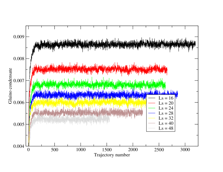
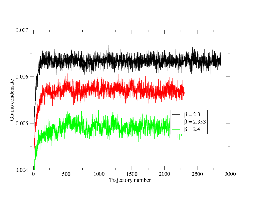
For each ensemble, a total of 700 to 1000 trajectories were generated starting from an ordered configuration, where all gauge link fields where set to unity. For these ensembles, equilibrium was achieved within the first trajectories. Approximately 1500 to 3000 trajectories where generated for the ensembles from an ordered start and thermalization was achieved within the first 500 to 700 trajectories. Specific thermalization times for these ensembles are indicated in Table 3 and Table 4. Measurements of observables were made using uncorrelated configurations which were generated thereafter. A plot of the gluino condensate time history is shown for a variety of couplings and values in Fig. 1 and Fig. 2 on lattices.
In order to correctly assess the statistical errors associated with various observable measurements, we first determine the integrated correlation time associated with the observable . This may be obtained from the normalized auto-correlation function , defined by:
| (75) |
where
| (76) |
The integrated correlation time associated with the observable is computed using:
| (77) |
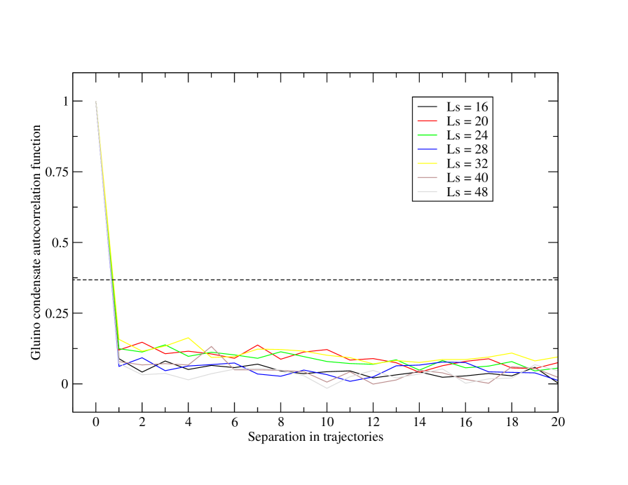
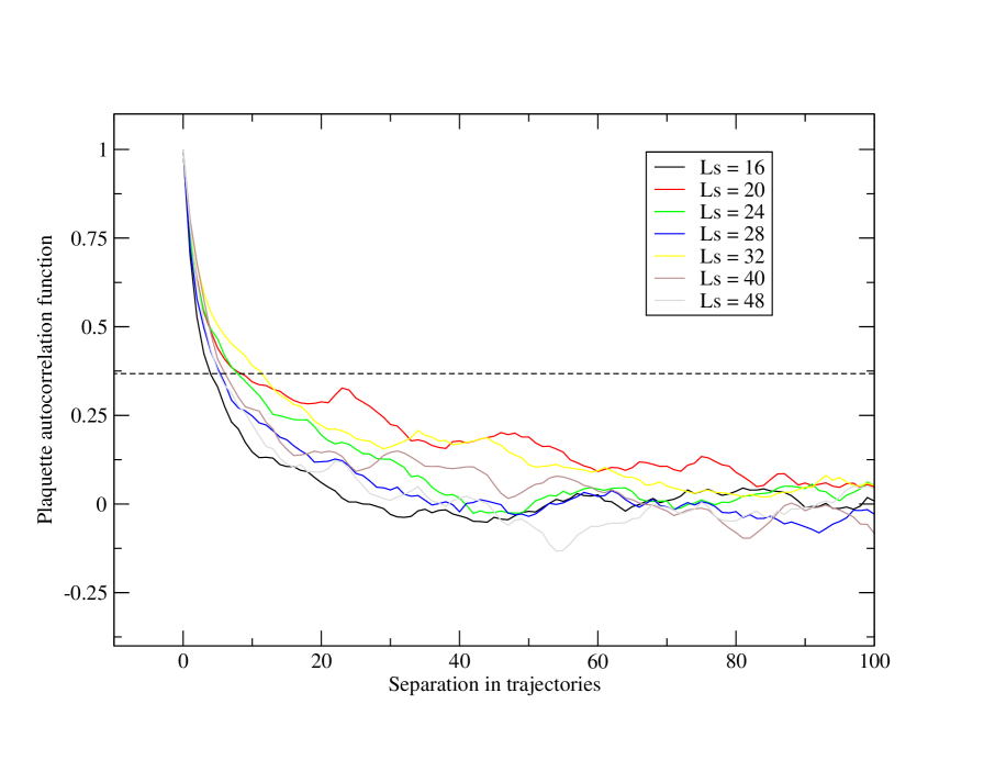
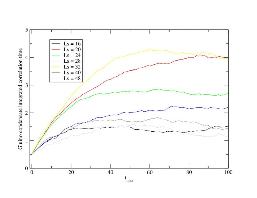
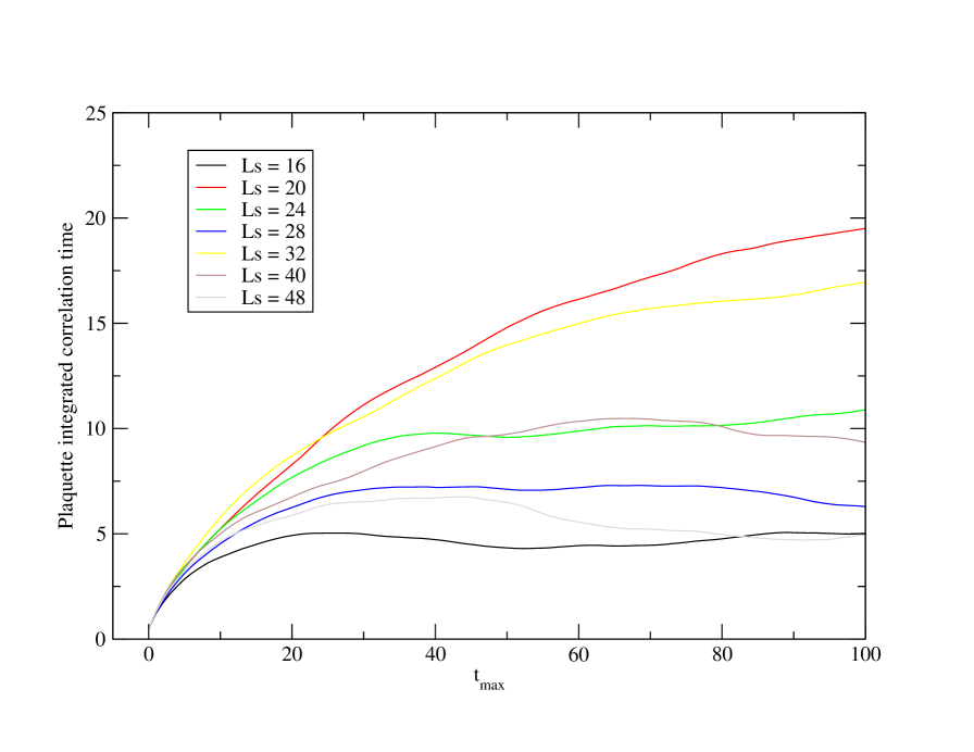
Figure 3 and Fig. 4 show the dependence of the auto-correlation function associated with the gluino condensate and average plaquette respectively. The exponential correlation time can be estimated from the value of at which . The integrated correlation time as a function of is plotted for these same observables in Fig. 5 and Fig. 6. Because the gluino condensate was measured using a stochastic estimator, one might expect decorrelation of this observable to occur relatively quickly in comparison to the average plaquette. However, the dependence of the integrated correlation time suggest that longer correlations are merely obscured by the presence of random noise.
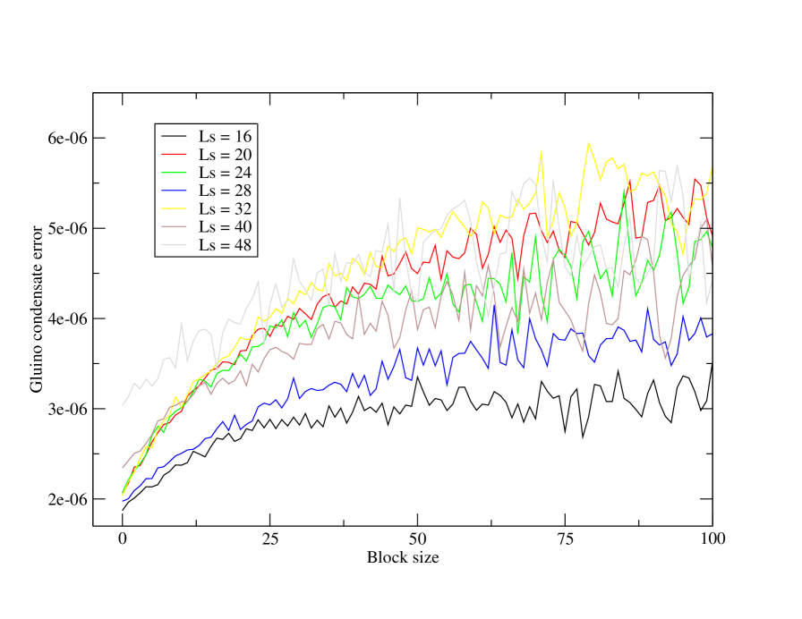
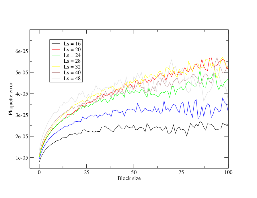
To better understand the correlations, we block our data with block size and consider the dependence of the errors on each observable. In Fig. 7 and Fig. 8 we plot the error as a function of block size for the gluino condensate and average plaquette. We find that for the gluino condensate, the decorrelation time is indeed much longer than what is implied by Fig. 3. Based on these considerations, we determine the gluino condensate and plaquette using a block size , where measurements have been made on every trajectory. For measurements of the static quark potential, we use a block size , where Wilson loops have been measured on every fifth trajectory. Unless otherwise noted, all other ensemble averages were performed using measurements made on every five trajectories.
IV Measurements, Analysis and Results
IV.1 Residual mass
Measurements of the residual mass where obtained from using Eq. 52 with wall gluino sources. The residual mass was computed from a constant fit of over the plateau region: 10-21. Fit results may be found in Table 7 and in Fig. 9. In the large limit, the residual mass is expected to behave as
| (78) |
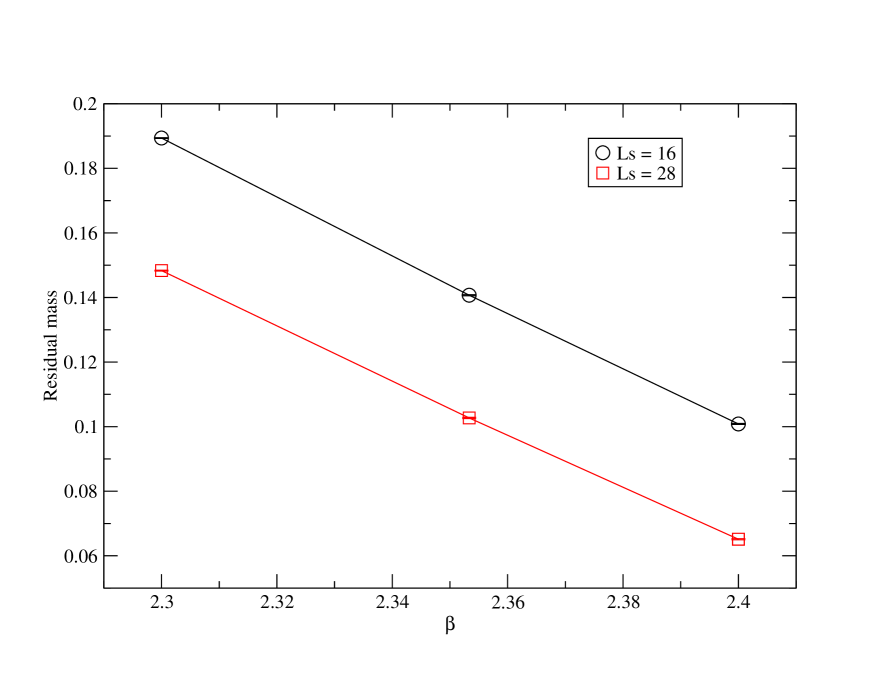
where the exponential term is a perturbative contribution which comes from extended modes above the mobility edge Antonio et al. (2008). The contribution to may be attributed to lattice dislocations and is proportional to the density of near unit modes of the five dimensional transfer matrix. For these simulations, the residual mass is roughly 5-20 times that of the input gluino mass. Figure 10 shows a plot of the residual mass as a function of the coupling. The strong coupling dependence of suggests that the dislocation contribution to the residual mass dominates over that of the perturbative part.
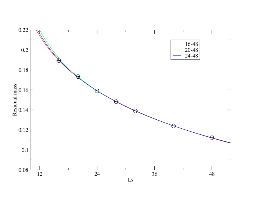
Figure 11 shows the dependence of the residual mass on at fixed coupling and . For and , we fit the residual mass as a function of using the functional form of Eq. 78. Fits were performed for a variety of different fit ranges in order to estimate the systematic errors associated with the fit. Results may be found in Table 8. These fits yield a negative value for the coefficient , which is inconsistent with the naíve expectation that should be positive. The naíve expectation, however, assumes that we are simulating the theory at couplings which are sufficiently close to the continuum limit so that the low energy identity Eq. 45 holds. Provided the underlying assumptions made in the calculation of are correct, one possible explanation for a negative value for is that higher order contributions to Eq. 39 have contaminated our estimate of the residual mass obtained from Eq. 52.
IV.2 Static potential
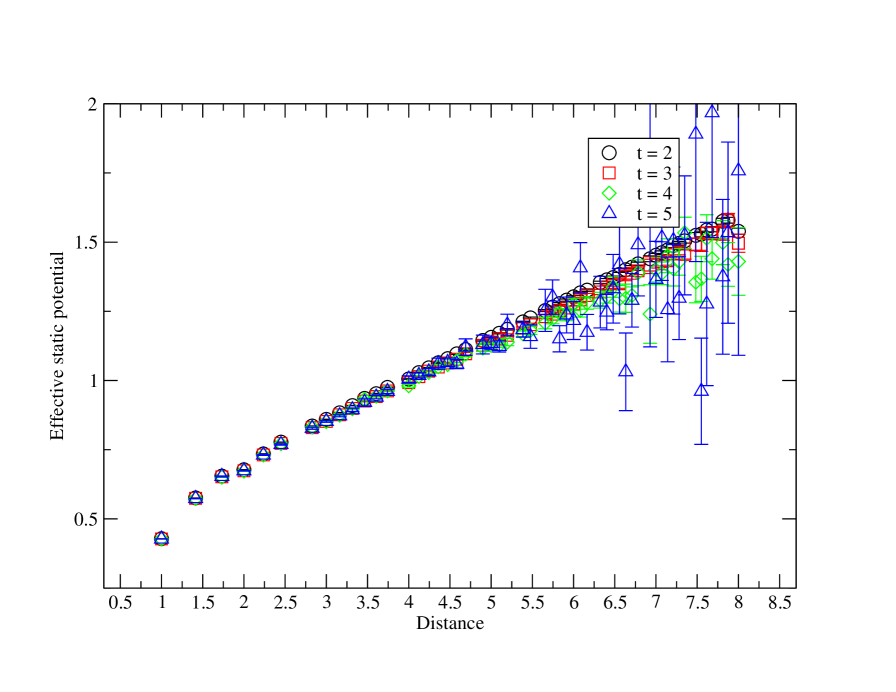
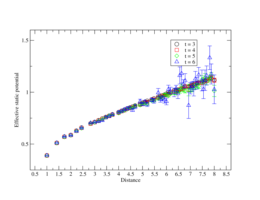
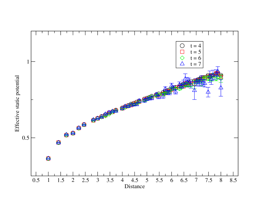
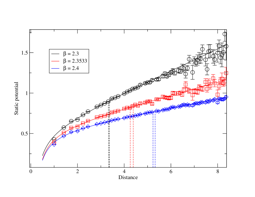
Here we describe the analysis of our static potential measurements. To begin, we first determined the plateau region of Eq. 53 over which excited state contamination becomes negligible by investigating the effective potential Eq. 54 as a function of distance for a variety of time slice values. Figure 12, Fig. 13 and Fig. 14 show the distance dependence of for each of the three values of , and with and . For , we take the plateau region to be the time range: 4-8, whereas for and we use the ranges: 5-9 or 5-10. For fixed distances , the Wilson loops were then fit as a function of time to the formula Eq. 53 within the previously determined time interval. Finally the extracted potentials were fit as a function of distance to the Cornell potential given by Eq. 55. Table 9 provides the fit results and respective errors which were determined by a jackknife analysis. Systematic errors in this fitting procedure may be estimated by varying the upper and lower limits of the fit ranges. These yield variations in the Sommer scale, however, which are comparable–if not smaller than–the statistical errors.
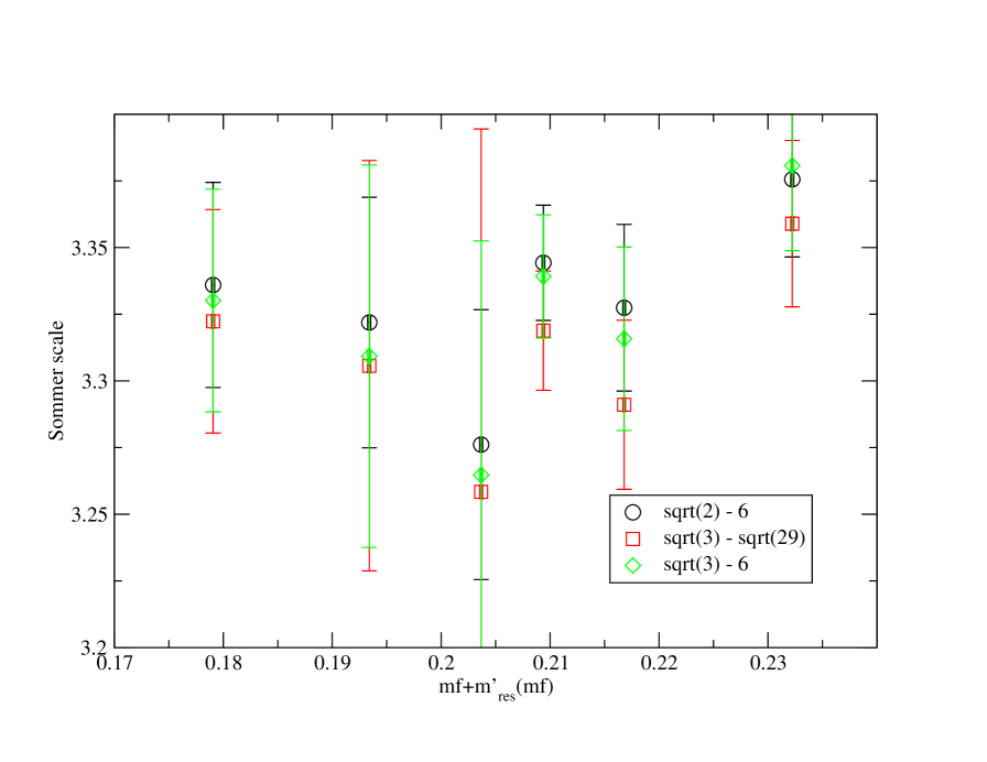
Figure 15 shows a plot of the static potential at the three different values of the coupling; the corresponding fit parameters may be found in Table 9. From and we determine the Sommer scale defined by Eq. 56.555Measurements of the Sommer scale were performed in collaboration with I. Mihailescu. As indicated in Table 9, the Sommer scale ranges from between for and for . Our static potential results provide evidence that the theory is confining, which is consistent with expectations. Figure 16 shows a plot of as a function of for . From this plot it appears that the Sommer scale has little discernible gluino mass dependence at the current level of statistics.
IV.3 Gluino condensate
In this section we describe the chiral limit extrapolation of the gluino condensate. This extrapolation requires taking both the and limits in some fashion. We begin by discussing the former.
For fixed , we fit the gluino condensate defined in Eq. 57 as a function of using the best available, theoretically motivated fit formula:
| (79) |
which is based upon the functional dependence of on . Note, however, that the dislocation contribution to which appears in Eq. 78 is absent in Eq. 79. The reason for this omission may be understood by observing that the chiral condensate is dominated by contributions from UV modes, whereas the dislocation term appearing in may predominantly be attributed to low energy phenomena Cheng (2008).
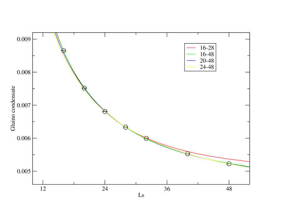
Before considering the chiral limit extrapolation of the condensate we investigate the dependence of the gluino condensate for and a fixed input gluino mass . The primary purpose of this investigation is two-fold. First, we would like to test our assumptions leading to Eq. 79 by checking that the fit value for is consistent with that of obtained in Eq. 78. Second, we wish to ascertain the systematic errors associated with an extrapolation of the condensate, which come from the limited range of values used in the fit. Results of our fits to Eq. 79 are provided in Table 10 and Fig. 17. From these fit results we conclude that the fit over the range: 16-28 overestimates the value of the chiral condensate at fixed by approximately 25% compared to our most reliable estimates which are obtained from the fit ranges: 20-48 and 24-48. We find large variations in the parameter with the fit range, however the results are within a factor of two of obtained from the residual mass extrapolations.
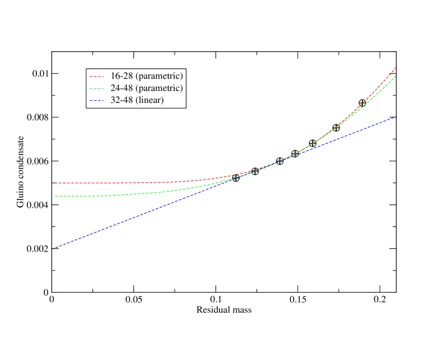
As an alternative approach, one may consider a linear extrapolation of the gluino condensate as a function of the residual mass, as was performed in Giedt et al. (2009), in order to obtain an value for the condensate at fixed . However such an approach assumes the same functional dependence on for both the condensate and the residual mass. While indeed for sufficiently large , each of these quantities will scale as and such a scenario may be achieved, for the values of used in this study, it is believed that the chiral condensate is dominated by a UV divergent term which is proportional to the perturbative contribution to the residual mass. Here, we compare the results of a linear extrapolation of the condensate as a function of the residual mass using the three data points which lie closest to the limit (i.e., and ). Results from this linear extrapolation are plotted in Fig. 18 and yield a condensate value of at . Also plotted in Fig. 18 are parametric plots of the gluino condensate as a function of the residual mass using Eq. 78, Eq. 79, and the fit parameters obtained in Table 8 and Table 10. Specifically we use the range: 24-48 fit parameters for and the range: 24-48 and 28-48 fit parameters for the condensate. A linear extrapolation of the condensate as a function of the residual mass yields a value which underestimates our extrapolation by approximately 100-150%.
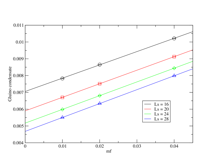
Finally we consider the chiral limit extrapolation of the condensate. Such an extrapolation may be achieved by considering the individual and dependence of the condensate, as was considered in Fleming et al. (2001). Here, we perform chiral limit extrapolations of the gluino condensate at a single lattice spacing () using two different limit orders. First, we perform a linear extrapolation of the gluino condensate at fixed using the formula
| (80) |
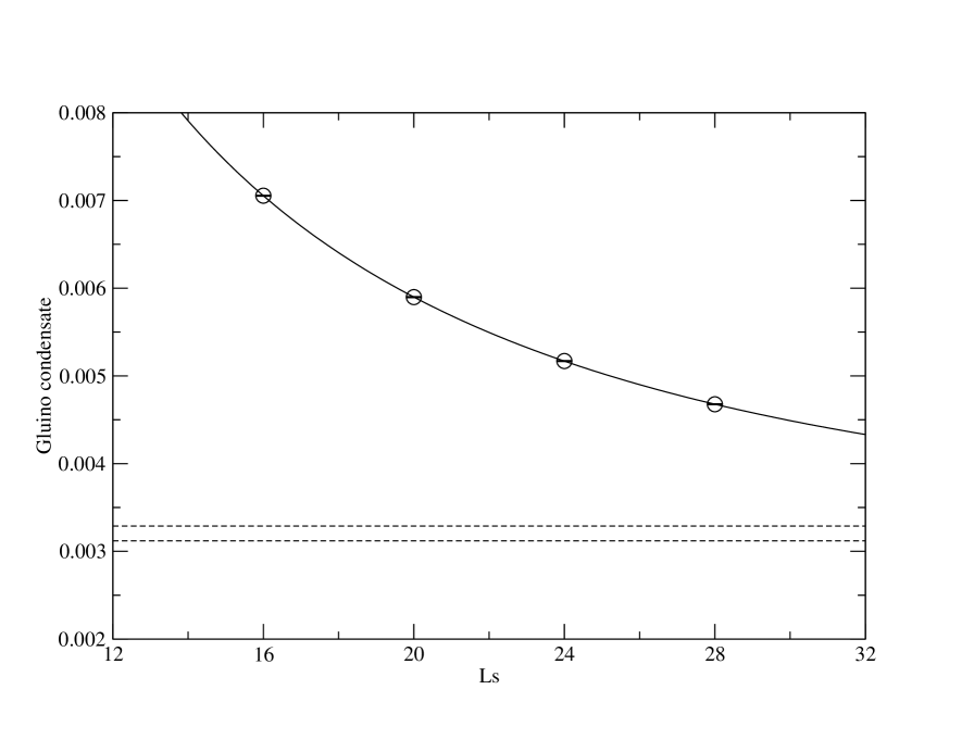
followed by an extrapolation of the result using Eq. 79. We believe that this approach is more transparent than, for instance, a linear extrapolation of the condensate as a function of (followed by a linear extrapolation), and most importantly, it correctly accounts for the functional form of Eq. 79.
Following the double extrapolation procedure outlined above, we obtain an unrenormalized value for the gluino condensate in the chiral limit at finite lattice spacing. Results from these fits are tabulated in Table 11 and Table 12 and plotted in Fig. 19 and Fig. 20, and yield the chiral limit value of 0.00320(9) for the condensate. Chiral extrapolations have also been performed by reversing the order of limits and yield consistent results with comparable statistical error bars. The fits of the condensate as a function of were performed over a fit range: 16-28 and, as such, we expect our chiral limit result to over estimate the true answer by approximately 25%, as was found for our extended fits at and , which are described above. We have performed additional fits using other, phenomenologically motivated fit formulae to describe the dependence of the gluino condensate (e.g., Eq. 79, without the prefactor in the second term). Such fits yield an approximate 20% variation in the chirally extrapolated value of the gluino condensate as compared to that obtained by using Eq. 79.
IV.4 Spectrum of the Hermitian DWF Dirac operator
Here we study the eigenvalues and eigenvectors of the Hermitian DWF Dirac operator. The primary purpose of this study is to establish to what degree the five dimensional theory reproduces the correct four-dimensional, continuum low energy physics and to obtain an independent measure of the residual mass and gluino condensate. To achieve this aim, we measure the lowest 64 eigenvalues and eigenvectors of the Hermitian DWF Dirac operator on lattices using the method of Kalkreuter-Simma (KS) Kalkreuter and Simma (1996). In this method, the Hermitian matrix is first diagonalized using a modified Rayleigh-Ritz diagonalization procedure, where we have exploited the relationship between degenerate eigenvectors and in order to eliminate any unnecessary minimizations of the Ritz functional. Subsequently, the matrix is diagonalized using Jacobi’s method within the subspace obtained from diagonalizing . These steps are then iterated until specified stopping criteria have been achieved. A detailed description of the procedure used to diagonalize and the stopping criteria may be found in Blum et al. (2002). For our purposes, the process was considered converged when the change in the eigenvalues between iterations was less than . We check this choice by increasing the stopping condition to on a test configuration and determined that eigenvalues changed by at most 0.02% over the the range of eigenvalues considered.
The eigenvectors of obtained from the KS method are ordered such that the magnitude of are ascending with eigenvector number. In all of the analysis that follows we use only the first 60 of the 64 eigenvalues obtained, since the last few may be unreliable Blum et al. (2002). Since there is a two-fold degeneracy in the spectrum due to Eq. 62, this yields a total of 30 non-degenerate eigenvectors and eigenvalues. All measurements in this work were performed on lattices with and a sea gluino mass: . In physical units, the lowest 60 eigenvalues for a typical configuration range roughly between for the ensembles and valence masses under consideration.
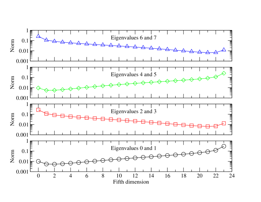
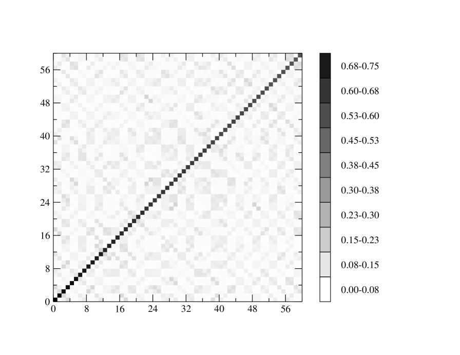
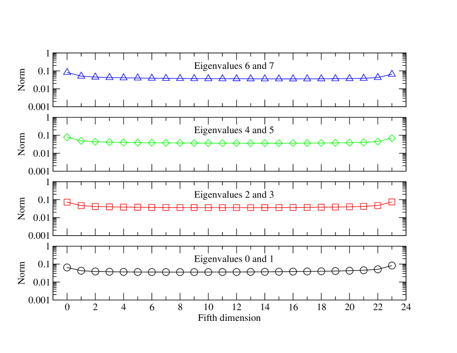
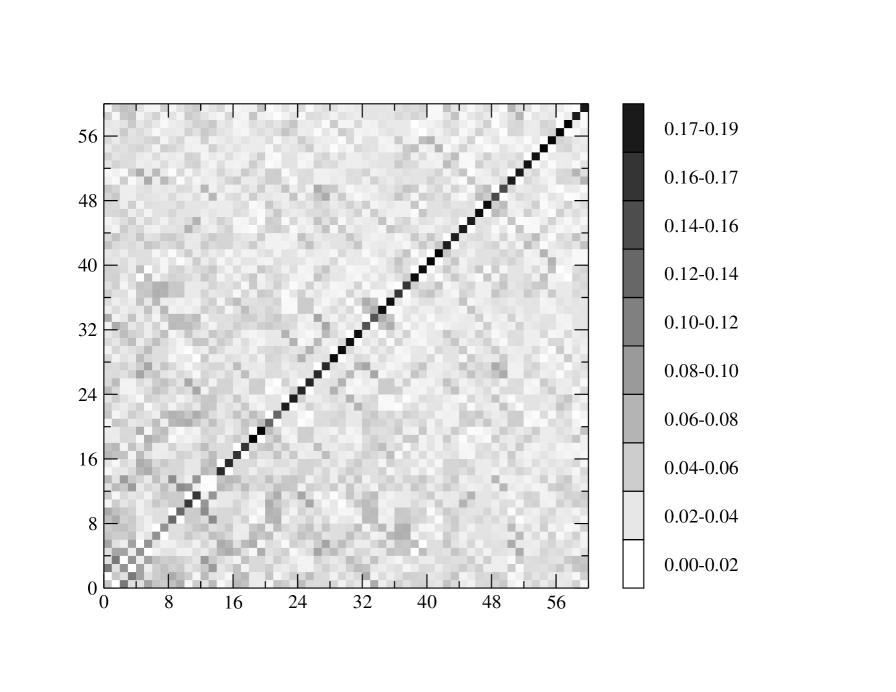
The lowest 60 eigenvectors were used to compute the matrix elements of the physical gamma matrix defined in Eq. 70, as well as to determine the localization of wave functions in the fifth dimension, which may be characterized by as defined in Eq. 69. Figure 21 and Fig. 22 shows the results of these calculations for a representative background gauge field configuration in the ensemble: , and , with . As may be seen in these figures, the eigenvectors are exponentially localized on both boundaries of the fifth dimension and alternate with increasing . The near-diagonal nature of confirms that the low-lying eigenvectors of are near chiral modes, however these states are not necessarily near-zero modes of . We find that in every instance:
| (81) |
which is entirely consistent with continuum predictions in the regime where , according to Eq. 64.
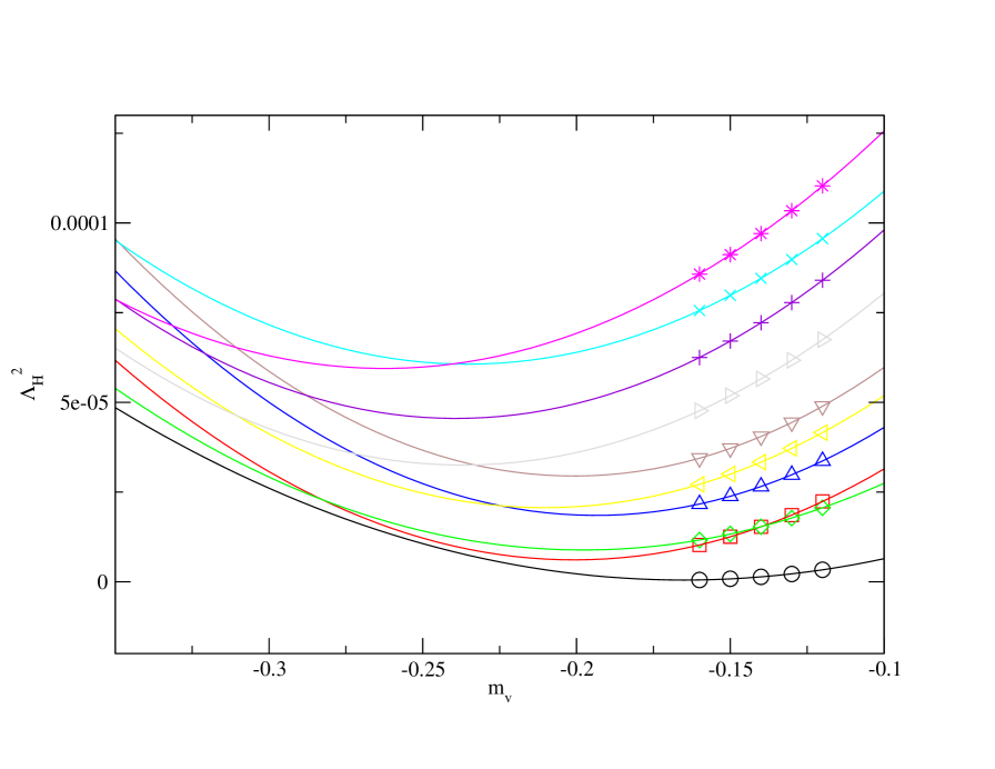
Next we study the dependence of and attempt to extract the residual mass and chiral condensate for the , , and , and ensembles. Eigenvalues were computed for five values of , ranging from to , on a total of gauge configurations. After appropriately reordering eigenvalues in order to account for possible level crossings, we fit the lowest 60 eigenvalues of as a function of to Eq. 71 and extract the parameters , and for each eigenvector. Figure 23 shows a plot of the fit results for the lowest 20 eigenvalues on a representative background field configuration for . As may be seen in this plot, for a typical eigenvector, the splitting of pairs due to the finite lattice spacing effects appear comparable to the spacings between adjacent eigenvectors. As a qualitative measure, we conclude that the lattice spacing is not sufficiently small for the emergence of this continuum behavior of the Dirac spectrum.
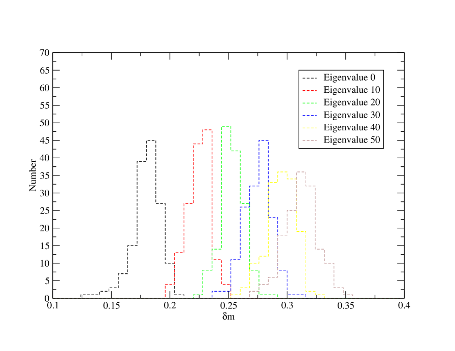
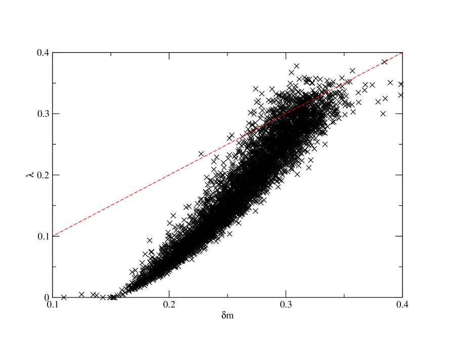
In Fig. 24 we plot the distribution of values at fixed eigenvalue number for the ensemble. Identifying the peak of the distribution of values with the residual mass relies on an assumption that the spectrum of is in some sense continuum-like. Unfortunately due to the lack of eigenvalue pairing, such interpretation is somewhat obscured. For the lowest eigenvalue, the mean of the distribution appears consistent with the value of obtained from Eq. 52, however for larger eigenvalues, the mean increases in magnitude.
In Fig. 25 we plot the values of verses for all eigenvalues, which were extracted from fits to Eq. 71 for the ensemble. At low energies, it is evident that we are in a regime where , which is consistent with our findings for the structure of in Fig. 22. If the distribution of is highly peaked about , one may in principle tune such that and expect off diagonal pairing to emerge in the matrix elements of . An attempt to produce off-diagonal pairing of by tuning was unsuccessful, but is likely due to the fact that off-diagonal pairing in may only occur when the eigenvalues of are paired. In Fig. 26 we plot for the same configuration as in Fig. 21, however with . Figure 27 displays the corresponding matrix elements of for this configuration. From the first plot, we see that the lowest lying wave functions are no longer strongly localized on the fifth dimension boundaries. As such, the diagonal structure of in Fig. 27 disappears for the lowest few modes, although off-diagonal pairing in not very evident either.
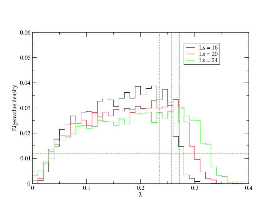
In Fig. 28 we plot the density of four dimensional eigenvalues for , and , which have been extracted from eigenvalue measurements using Eq. 71. The distribution exhibits a relatively constant region between and , and a depleted region between and which may be attributed to finite volume effects. Contrary to continuum expectations, there is no visible peak at , which one would normally attribute to near-zero modes. If such a peak were to exist, it may be that its height is suppressed due to a finite bin size , which is too large. From Fig. 23, however, it appears that the number of zero modes is few, suggesting that there is perhaps little topology change and that we are primarily within the zero topological charge sector of the theory. This observation is consistent with the findings of Fleming et al. (2001), where fluctuations in the condensate as a function of MD time where studied as a possible indicator of topology change. In that study, no large spikes in evolution of the condensate (which would correspond to the presence of zero-modes) were observed for the same choice of parameters. Yet in light of the fact that the residual mass is so large in these simulations, it may also be that the fermions simply provide a poor measure of topology. To make a more definitive statement regarding the topic, it would be interesting and beneficial to study the gauge fields directly instead.
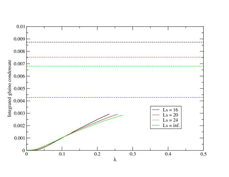
In principle one may extract an estimate of from the constant region of the eigenvalue density, compute the condensate and finally perform an extrapolation. But for the current choice of simulation parameters, the low lying spectrum appears to be too heavily distorted by the large residual mass for such an analysis to be reliable. We may still extract some useful information from the eigenvalue density, however. In our analysis of the chiral extrapolation of the gluino condensate described in Sec. IV.3, we assumed that the dependent contribution to the condensate was dominated by UV modes. We may check this assumption, by computing the contribution to Eq. 57 from modes in the interval: -, using our fit values for and and Eq. 72 with . In Fig. 29, we plot the integrated condensate as a function of the upper limit value for , and . The contribution to the condensate from modes is approximately of the total value for each choice of , which is consistent with our assumptions.
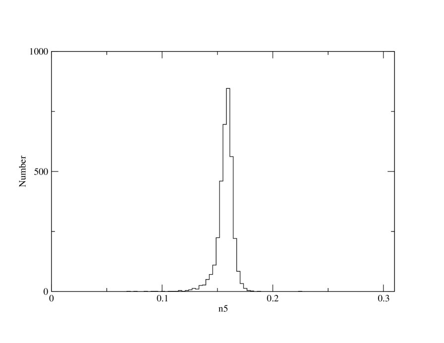
Finally for completeness, Fig. 30 provides a histogram of values extracted from the fits for the , and ensemble, where it is evident that is strongly peaked at approximately .
V Conclusion
We have performed dynamical numerical simulations of N=1 SYM theory on and lattices using domain wall fermions with several goals in mind: to establish a lattice scale, assess the size of chiral symmetry breaking effects at finite , and understand the degree to which DWFs are correctly reproducing the desired continuum physics at low energy. In part, these efforts were motivated by the necessity to establish benchmarks for future studies. As such, our work consists of a variety of basic measurements on lattices, including measurements of the static potential, residual mass and gluino condensate. We buttress these results by analyzing the eigenvalues and eigenvectors of the Hermitian DWF Dirac operator on lattices, from which an independent estimate of the residual mass and chiral condensate may in principle be extracted. We briefly summarize each of our measurements and results below.
We have presented results for the residual mass, which have been obtained using two different methods. The first approach utilized a low energy identity relating the wall pseudo-scalar density to the midpoint pseudo-scalar density and assumptions about the decomposition of connected and disconnect parts of various pseudo-scalar correlators. Using this approach we obtained residual masses which where approximately 5-20 times larger than the input gluino mass . A second approach for obtaining , based upon the dependence of the eigenvalues of , gave inconclusive yet qualitatively consistent results for the residual mass. On an eigenvalue by eigenvalue basis, chiral symmetry breaking shifts in where comparable, if not larger than the value for obtained in the first approach. The limited success of the second method in determining a precise value for the residual mass may be attributed to large finite lattice spacing artifacts.
The static potential for fundamental representation sources was determined using standard techniques for three different values of the coupling. The potential exhibits characteristics indicative of confinement. From the static potential we obtain estimates of the Sommer scale, which range from approximately at to at .
We study properties of the low energy eigenvalues of the Hermitian DWF Dirac operator in an effort to understand to what degree the desired low energy physics is reproduced by the DWF formalism. By studying the profile of the wave functions as a function of the fifth dimension coordinate, we have established that the low energy modes are indeed localized on the right and left boundaries of the fifth direction. And, the matrix elements of the physical chirality operator are consistent with the presence of a large gluino mass compared to the typical low energy eigenvalues of .
We have performed a chiral extrapolation of the gluino condensate at a fixed value of the lattice spacing, . The chiral extrapolation of the condensate was performed in a variety of different ways in order to elucidate some of the systematic errors inherent with the extrapolation. For the parameters under consideration we find that various extrapolation procedures yield, at best, a value of the condensate which is reliable to approximately 25%. We attempt to provide an independent measurement of the gluino condensate from our studies of the Dirac spectrum. However, given the current large values of the residual mass, a reliable estimate of the gluino condensate from the Banks-Casher relation was not possible.
Finally, we come to the general conclusion that there is, at present, no evidence to suggest that our simulations are not in the same universality class as SYM at non-zero gluino mass. However, additional simulations will be required at far smaller residual masses and weaker couplings in order to achieve a more reliable measure of the quantities discussed in this paper. Reducing the residual mass may be achieved with a variety of approaches; the simplest approach is to increase the size of the fifth dimension. This method for reducing the residual mass becomes costly, however, once the dislocation term appearing in Eq. 78 dominates over the perturbative contribution to the residual mass. Alternatives to this approach, which may be more efficient, include going to weaker coupling, or using an improved action such as the DBW2 de Forcrand et al. (2000), Iwasaki Iwasaki and Yoshie (1984); Iwasaki (1985), or auxiliary determinant Renfrew et al. (2009) action. The latter action combines the Gap DWF method of Vranas (1999, 2006) with the approach of Fukaya et al. (2006) in order to suppress the residual mass while still maintaining adequate topological tunneling. Such considerations will be left to a future study. Finally we emphasis that scaling analysis at weaker coupling is essential in order to truly understanding the effects of finite lattice spacing on observables, and whether or not the gluino condensate survives the continuum limit.
Acknowledgements.
M. G. E. would like to thank T. Blum, N. Christ, C. Dawson, C. Kim, R. Mawhinney and S. Takeda for helpful discussions, I. Mihailescu for fitting the static potential data presented in this work, and C. Jung for technical assistance with compiling and running the Columbia Physics System on BlueGene/L and QCDOC. This research utilized resources at the New York Center for Computational Sciences at Stony Brook University/Brookhaven National Laboratory which is supported by the U.S. Department of Energy under Contract No. DE-AC02-98CH10886 and by the State of New York. Early portions of this work were performed on QCDOC at Columbia University. This work was supported by the U.S. Department of Energy under grant number DE-FG02-92ER40699.Appendix A Correlators involving Majorana fermions
In SYM, the fundamental fermionic degrees of freedom are Majorana fermions rather than Dirac fermions. As a result, correlation functions written in terms of propagator contractions may differ from that of conventional QCD. Here we briefly review the construction of some of the basic observables studied in the paper, although for simplicity we limit the majority of the discussion to four dimensions. Generalization of the results to the specific case of DWFs will be considered at the end of this section.
To begin with, consider the generic Majorana fermion path integral:
| (82) |
where the indices for collectively represent space-time coordinate (), spin () and color (), and summation over these indices is implied. Due to the anti-commuting nature of the variables , components of which are symmetric under the interchange of any two indices will not contribute to . The Majorana matrix is related to the Dirac operator via the relation , where is the charge conjugation matrix whose properties in four dimension are given in Eq. 17. We allow the Dirac operator and to depend on background field configurations and, as such, so may the normalization factor . By definition we choose such that , and so it follows that . Expectation values of operators involving the fermion fields in the full gauge theory are given by gauge averages over with the probability measure , where is the gauge action.
The path integral given by Eq. 82 may be evaluated in a standard fashion, and yields
| (83) |
where
| (87) |
is the Pfaffian constructed from Majorana propagators , which start and end on the points in all possible combinations. Note that since the matrix is antisymmetric, the diagonal matrix elements of the propagator vanish.
As an example of how this result may be applied, consider the two important cases and , for which:
| (88) | |||||
| (89) |
In the case of the condensate defined in Eq. 57, we have:
| (90) |
which according to the expression for in Eq. 89 yields:
| (91) |
prior to gauge averaging. Here, is the Dirac propagator and the trace is taken over both spin and color. In the case of the pseudo-scalar correlator , where , we have
| (92) |
which according to the expression for in Eq. 89 yields:
| (93) |
prior to gauge averaging. Note that the connected and disconnected parts of this correlator, as defined in Eq. 48, correspond to the single and double trace terms respectively.
While the results presented here pertain to the four dimensional theory, they may easily be generalized to the case of DWFs, where the interpolating gluino fields are expressed in terms of the fields at the fifth dimension boundary, according to Eq. 20. Specifically the results for the gluino condensate and pseudo-scalar correlator given by Eq. 91 and Eq. 93 remain valid with the simple replacement , where
| (95) | |||||
and is the DWF Dirac operator defined in Eq. 3.
References
- Feo (2003) A. Feo, Nucl. Phys. Proc. Suppl. 119, 198 (2003), eprint hep-lat/0210015.
- Giedt (2006) J. Giedt, PoS LAT2006, 008 (2006), eprint hep-lat/0701006.
- Witten (1997) E. Witten, Nucl. Phys. B507, 658 (1997), eprint hep-th/9706109.
- Witten (1982) E. Witten, Nucl. Phys. B202, 253 (1982).
- Veneziano and Yankielowicz (1982) G. Veneziano and S. Yankielowicz, Phys. Lett. B113, 231 (1982).
- Farrar et al. (1998) G. R. Farrar, G. Gabadadze, and M. Schwetz, Phys. Rev. D58, 015009 (1998), eprint hep-th/9711166.
- Ginsparg and Wilson (1982) P. H. Ginsparg and K. G. Wilson, Phys. Rev. D25, 2649 (1982).
- Neuberger (1998) H. Neuberger, Phys. Lett. B417, 141 (1998), eprint hep-lat/9707022.
- Kaplan (1992) D. B. Kaplan, Phys. Lett. B288, 342 (1992), eprint hep-lat/9206013.
- Narayanan and Neuberger (1993) R. Narayanan and H. Neuberger, Phys. Lett. B302, 62 (1993), eprint hep-lat/9212019.
- Shamir (1993) Y. Shamir, Nucl. Phys. B406, 90 (1993), eprint hep-lat/9303005.
- Campos et al. (1999) I. Campos et al. (DESY-Munster), Eur. Phys. J. C11, 507 (1999), eprint hep-lat/9903014.
- Farchioni et al. (2002) F. Farchioni et al. (DESY-Munster-Roma), Eur. Phys. J. C23, 719 (2002), eprint hep-lat/0111008.
- Montvay (2002) I. Montvay, Int. J. Mod. Phys. A17, 2377 (2002), eprint hep-lat/0112007.
- Montvay (2000) I. Montvay, Nucl. Phys. Proc. Suppl. 83, 188 (2000), eprint hep-lat/9909020.
- Feo et al. (2000a) A. Feo, R. Kirchner, S. Luckmann, I. Montvay, and G. Munster (DESY-Munster), Nucl. Phys. Proc. Suppl. 83, 661 (2000a), eprint hep-lat/9909070.
- Peetz et al. (2003) R. Peetz, F. Farchioni, C. Gebert, and G. Munster, Nucl. Phys. Proc. Suppl. 119, 912 (2003), eprint hep-lat/0209065.
- Farchioni et al. (2004) F. Farchioni, G. Muenster, and R. Peetz, Eur. Phys. J. C38, 329 (2004), eprint hep-lat/0404004.
- Farchioni and Peetz (2005) F. Farchioni and R. Peetz, Eur. Phys. J. C39, 87 (2005), eprint hep-lat/0407036.
- Koutsoumbas et al. (1998) G. Koutsoumbas et al., Nucl. Phys. Proc. Suppl. 63, 727 (1998), eprint hep-lat/9709091.
- Kirchner et al. (1999) R. Kirchner, I. Montvay, J. Westphalen, S. Luckmann, and K. Spanderen (DESY-Munster), Phys. Lett. B446, 209 (1999), eprint hep-lat/9810062.
- Feo et al. (2000b) A. Feo, R. Kirchner, I. Montvay, and A. Vladikas (DESY-Munster), Nucl. Phys. Proc. Suppl. 83, 670 (2000b), eprint hep-lat/9909071.
- Montvay (1996) I. Montvay, Nucl. Phys. B466, 259 (1996), eprint hep-lat/9510042.
- Donini and Guagnelli (1996) A. Donini and M. Guagnelli, Phys. Lett. B383, 301 (1996), eprint hep-lat/9605010.
- Koutsoumbas and Montvay (1997) G. Koutsoumbas and I. Montvay, Phys. Lett. B398, 130 (1997), eprint hep-lat/9612003.
- Montvay (1997) I. Montvay, Nucl. Phys. Proc. Suppl. 53, 853 (1997), eprint hep-lat/9607035.
- Donini et al. (1998) A. Donini, M. Guagnelli, P. Hernandez, and A. Vladikas, Nucl. Phys. B523, 529 (1998), eprint hep-lat/9710065.
- Montvay (1998) I. Montvay, Nucl. Phys. Proc. Suppl. 63, 108 (1998), eprint hep-lat/9709080.
- Demmouche et al. (2008) K. Demmouche et al. (2008), eprint 0810.0144.
- Kaplan and Schmaltz (2000) D. B. Kaplan and M. Schmaltz, Chin. J. Phys. 38, 543 (2000), eprint hep-lat/0002030.
- Fleming et al. (2001) G. T. Fleming, J. B. Kogut, and P. M. Vranas, Phys. Rev. D64, 034510 (2001), eprint hep-lat/0008009.
- Gottlieb et al. (1987) S. A. Gottlieb, W. Liu, D. Toussaint, R. L. Renken, and R. L. Sugar, Phys. Rev. D35, 2531 (1987).
- Clark and Kennedy (2004) M. A. Clark and A. D. Kennedy, Nucl. Phys. Proc. Suppl. 129, 850 (2004), eprint hep-lat/0309084.
- Clark et al. (2005) M. A. Clark, A. D. Kennedy, and Z. Sroczynski, Nucl. Phys. Proc. Suppl. 140, 835 (2005), eprint hep-lat/0409133.
- Clark et al. (2006) M. A. Clark, P. de Forcrand, and A. D. Kennedy, PoS LAT2005, 115 (2006), eprint hep-lat/0510004.
- Giedt et al. (2009) J. Giedt, R. Brower, S. Catterall, G. T. Fleming, and P. Vranas, Phys. Rev. D79, 025015 (2009), eprint 0810.5746.
- Giedt et al. (2008) J. Giedt, R. Brower, S. Catterall, G. T. Fleming, and P. Vranas (2008), eprint 0807.2032.
- Banks and Casher (1980) T. Banks and A. Casher, Nucl. Phys. B169, 103 (1980).
- Endres (2008) M. G. Endres (2008), eprint 0810.0431.
- Furman and Shamir (1995) V. Furman and Y. Shamir, Nucl. Phys. B439, 54 (1995), eprint hep-lat/9405004.
- Vranas (1998) P. M. Vranas, Phys. Rev. D57, 1415 (1998), eprint hep-lat/9705023.
- Shamir (1994) Y. Shamir, Nucl. Phys. B417, 167 (1994), eprint hep-lat/9310006.
- Allton et al. (2007) C. Allton et al. (RBC and UKQCD), Phys. Rev. D76, 014504 (2007), eprint hep-lat/0701013.
- Omelyan et al. (2003) I. Omelyan, I. Mryglod, and R. Folk, Comput. Phys. Commun. 151, 272 (2003).
- Takaishi and de Forcrand (2006) T. Takaishi and P. de Forcrand, Phys. Rev. E73, 036706 (2006), eprint hep-lat/0505020.
- Creutz (1988) M. Creutz, Phys. Rev. D38, 1228 (1988).
- Sommer (1994) R. Sommer, Nucl. Phys. B411, 839 (1994), eprint hep-lat/9310022.
- Blum et al. (2004) T. Blum et al., Phys. Rev. D69, 074502 (2004), eprint hep-lat/0007038.
- Leutwyler and Smilga (1992) H. Leutwyler and A. V. Smilga, Phys. Rev. D46, 5607 (1992).
- Antonio et al. (2008) D. J. Antonio et al. (RBC), Phys. Rev. D77, 014509 (2008), eprint 0705.2340.
- Cheng (2008) M. Cheng (RBC), PoS LATTICE2008, 180 (2008), eprint 0810.1311.
- Kalkreuter and Simma (1996) T. Kalkreuter and H. Simma, Comput. Phys. Commun. 93, 33 (1996), eprint hep-lat/9507023.
- Blum et al. (2002) T. Blum et al., Phys. Rev. D65, 014504 (2002), eprint hep-lat/0105006.
- de Forcrand et al. (2000) P. de Forcrand et al. (QCD-TARO), Nucl. Phys. B577, 263 (2000), eprint hep-lat/9911033.
- Iwasaki and Yoshie (1984) Y. Iwasaki and T. Yoshie, Phys. Lett. B143, 449 (1984).
- Iwasaki (1985) Y. Iwasaki, Nucl. Phys. B258, 141 (1985).
- Renfrew et al. (2009) D. Renfrew, T. Blum, N. Christ, R. Mawhinney, and P. Vranas (2009), eprint 0902.2587.
- Vranas (1999) P. M. Vranas (1999), eprint hep-lat/0001006.
- Vranas (2006) P. M. Vranas, Phys. Rev. D74, 034512 (2006), eprint hep-lat/0606014.
- Fukaya et al. (2006) H. Fukaya et al. (JLQCD), Phys. Rev. D74, 094505 (2006), eprint hep-lat/0607020.
| 2.3 | 12 | 0.02 | 4.0 | 9 | 15 | 4.0 | 6 | 9 | ||
| 16 | 0.02 | 4.0 | 9 | 15 | 4.0 | 6 | 9 | |||
| 20 | 0.02 | 4.0 | 9 | 15 | 4.0 | 6 | 9 | |||
| 24 | 0.02 | 4.0 | 9 | 15 | 4.0 | 6 | 9 |
| 2.3 | 16 | 0.01 | 4.0 | 9 | 15 | 4.0 | 6 | 9 | ||
| 0.02 | 4.0 | 9 | 15 | 4.0 | 6 | 9 | ||||
| 0.04 | 4.0 | 9 | 15 | 4.0 | 6 | 9 | ||||
| 20 | 0.01 | 4.0 | 9 | 15 | 4.0 | 6 | 9 | |||
| 0.02 | 4.0 | 9 | 15 | 4.0 | 6 | 9 | ||||
| 0.04 | 4.0 | 9 | 15 | 4.0 | 6 | 9 | ||||
| 24 | 0.01 | 4.0 | 9 | 15 | 4.0 | 6 | 9 | |||
| 0.02 | 4.0 | 9 | 15 | 4.0 | 6 | 9 | ||||
| 0.04 | 4.0 | 9 | 15 | 4.0 | 6 | 9 | ||||
| 28 | 0.01 | 4.0 | 9 | 15 | 4.0 | 6 | 9 | |||
| 0.02 | 4.0 | 9 | 15 | 4.0 | 6 | 9 | ||||
| 0.04 | 4.0 | 9 | 15 | 4.0 | 6 | 9 | ||||
| 32 | 0.02 | 4.0 | 9 | 15 | 4.0 | 6 | 9 | |||
| 40 | 0.02 | 4.0 | 9 | 15 | 4.0 | 6 | 9 | |||
| 48 | 0.02 | 4.0 | 9 | 15 | 4.0 | 6 | 9 | |||
| 16 | 0.02 | 4.0 | 9 | 15 | 4.0 | 6 | 9 | |||
| 28 | 0.02 | 4.0 | 9 | 15 | 4.0 | 6 | 9 | |||
| 2.4 | 16 | 0.02 | 4.0 | 9 | 15 | 4.0 | 6 | 9 | ||
| 28 | 0.02 | 4.0 | 9 | 15 | 4.0 | 6 | 9 |
| Accept | |||||||||
|---|---|---|---|---|---|---|---|---|---|
| 2.3 | 12 | 0.02 | 0.260 | 1000 | 300 | 0.626(18) | 0.498(28) | 1.095(27) | 0.956(39) |
| 16 | 0.02 | 0.220 | 750 | 300 | 0.749(20) | 0.146(26) | 0.577(19) | 1.004(19) | |
| 20 | 0.02 | 0.240 | 1000 | 300 | 0.594(18) | 0.541(39) | 1.165(30) | 1.013(60) | |
| 24 | 0.02 | 0.230 | 1000 | 300 | 0.627(18) | 0.470(35) | 1.965(43) | 0.966(42) |
. Accept 2.3 16 0.01 0.160 3125 500 0.758(19) 0.193(28) 0.673(9) 1.016(14) 0.02 0.160 3195 500 0.762(18) 0.187(26) 0.625(8) 0.991(12) 0.04 0.160 2790 500 0.776(19) 0.152(26) 0.577(8) 1.003(12) 20 0.01 0.155 2895 500 0.745(20) 0.208(30) 0.685(10) 1.008(15) 0.02 0.155 2655 500 0.753(21) 0.212(31) 0.674(10) 0.993(16) 0.04 0.160 2760 500 0.731(21) 0.238(32) 0.722(11) 0.995(16) 24 0.01 0.155 2855 500 0.775(19) 0.142(26) 0.578(8) 1.019(13) 0.02 0.130 2620 500 0.792(20) 0.143(28) 0.593(11) 1.020(14) 0.04 0.155 2610 500 0.760(21) 0.175(32) 0.690(10) 1.050(17) 28 0.01 0.135 2740 500 0.817(18) 0.086(22) 0.474(7) 1.022(11) 0.02 0.140 2855 500 0.796(19) 0.158(24) 0.536(7) 0.974(11) 0.04 0.155 2880 500 0.784(19) 0.157(25) 0.577(8) 0.996(12) 32 0.02 0.140 2730 500 0.757(20) 0.180(29) 0.654(9) 1.016(15) 40 0.02 0.140 2189 500 0.628(27) 0.455(51) 1.028(18) 0.974(27) 48 0.02 0.140 1555 500 0.608(34) 0.586(76) 1.247(25) 1.031(46) 16 0.02 0.163 2575 600 0.782(20) 0.160(27) 0.583(9) 0.996(13) 28 0.02 0.140 2305 600 0.829(20) 0.072(22) 0.415(7) 1.012(10) 2.4 16 0.02 0.160 2710 750 0.824(18) 0.093(20) 0.432(7) 0.996(10) 28 0.02 0.140 2285 750 0.882(18) 0.040(18) 0.320(6) 1.010(8)
| 2.3 | 12 | 0.02 | 0.010631(40) | 0.73496(36) | |
|---|---|---|---|---|---|
| 16 | 0.02 | 0.008736(42) | 0.73296(51) | ||
| 20 | 0.02 | 0.007522(37) | 0.73276(30) | ||
| 24 | 0.02 | 0.006806(34) | 0.73202(32) |
| 2.3 | 16 | 0.01 | 0.0078277(43) | 0.733463(33) | |
|---|---|---|---|---|---|
| 0.02 | 0.0086506(30) | 0.733218(24) | |||
| 0.04 | 0.0102120(41) | 0.733203(36) | |||
| 20 | 0.01 | 0.0067032(46) | 0.732618(36) | ||
| 0.02 | 0.0075158(46) | 0.732530(57) | |||
| 0.04 | 0.0091267(35) | 0.732419(31) | |||
| 24 | 0.01 | 0.0059855(40) | 0.732127(35) | ||
| 0.02 | 0.0068081(42) | 0.732110(41) | |||
| 0.04 | 0.0084396(36) | 0.731983(37) | |||
| 28 | 0.01 | 0.0055027(46) | 0.731734(34) | ||
| 0.02 | 0.0063346(33) | 0.731688(32) | |||
| 0.04 | 0.0079882(32) | 0.731628(38) | |||
| 32 | 0.02 | 0.0059947(47) | 0.731418(45) | ||
| 40 | 0.02 | 0.0055266(43) | 0.730947(44) | ||
| 48 | 0.02 | 0.0052238(43) | 0.730727(50) | ||
| 16 | 0.02 | 0.0077917(72) | 0.745243(40) | ||
| 28 | 0.02 | 0.0057106(61) | 0.743853(38) | ||
| 2.4 | 16 | 0.02 | 0.0068851(64) | 0.754149(30) | |
| 28 | 0.02 | 0.0049179(82) | 0.752951(27) |
| time range | |||||
| 2.3 | 16 | 0.01 | 10-21 | 63.8/11 | 0.18682(13) |
| 0.02 | 10-21 | 15.0/11 | 0.18939(12) | ||
| 0.04 | 10-21 | 17.2/11 | 0.19223(13) | ||
| 20 | 0.01 | 10-21 | 10.8/11 | 0.17151(14) | |
| 0.02 | 10-21 | 35.1/11 | 0.17340(14) | ||
| 0.04 | 10-21 | 49.4/11 | 0.17680(13) | ||
| 24 | 0.01 | 10-21 | 13.4/11 | 0.15807(13) | |
| 0.02 | 10-21 | 18.4/11 | 0.15906(15) | ||
| 0.04 | 10-21 | 19.8/11 | 0.16367(13) | ||
| 28 | 0.01 | 10-21 | 28.6/11 | 0.14685(13) | |
| 0.02 | 10-21 | 25.5/11 | 0.14834(13) | ||
| 0.04 | 10-21 | 111.7/11 | 0.15283(13) | ||
| 32 | 0.02 | 10-21 | 5.1/11 | 0.13905(14) | |
| 40 | 0.02 | 10-21 | 23.2/11 | 0.12397(14) | |
| 48 | 0.02 | 10-21 | 29.1/11 | 0.11225(16) | |
| 16 | 0.02 | 10-21 | 45.5/11 | 0.14071(19) | |
| 28 | 0.02 | 10-21 | 42.5/11 | 0.10269(18) | |
| 2.4 | 16 | 0.02 | 10-21 | 9.5/11 | 0.10082(15) |
| 28 | 0.02 | 10-21 | 24.6/11 | 0.06513(17) |
| range | ||||||
|---|---|---|---|---|---|---|
| 2.3 | 16-48 | 0.02 | 53.5/4 | -6.20(3) | 0.0275(4) | 7.03(5) |
| 20-48 | 5.9/3 | -6.37(7) | 0.0236(7) | 7.43(10) | ||
| 24-48 | 2.2/2 | -6.30(5) | 0.0255(11) | 7.24(12) |
| time range | distance range | |||||||
| 2.3 | 16 | 0.02 | 4-8 | -6 | 0.511(10) | 0.176(10) | 0.132(2) | 3.344(21) |
| 0.02 | 4-8 | - | 0.483(17) | 0.140(23) | 0.137(4) | 3.319(22) | ||
| 0.02 | 4-8 | -6 | 0.501(18) | 0.161(23) | 0.134(4) | 3.339(23) | ||
| 0.04 | 4-8 | -6 | 0.524(15) | 0.185(14) | 0.129(3) | 3.376(29) | ||
| 0.04 | 4-8 | - | 0.516(26) | 0.178(33) | 0.130(5) | 3.381(32) | ||
| 0.04 | 4-8 | -6 | 0.534(26) | 0.200(32) | 0.127(5) | 3.359(31) | ||
| 20 | 0.02 | 4-8 | -6 | 0.511(13) | 0.174(13) | 0.134(4) | 3.322(47) | |
| 0.02 | 4-8 | - | 0.480(44) | 0.132(54) | 0.139(11) | 3.306(77) | ||
| 0.02 | 4-8 | -6 | 0.483(41) | 0.136(49) | 0.138(10) | 3.309(71) | ||
| 0.04 | 4-8 | -6 | 0.532(15) | 0.197(15) | 0.131(4) | 3.327(31) | ||
| 0.04 | 4-8 | - | 0.485(26) | 0.136(31) | 0.140(5) | 3.291(31) | ||
| 0.04 | 4-8 | -6 | 0.507(27) | 0.163(32) | 0.135(5) | 3.316(34) | ||
| 24 | 0.02 | 4-8 | -6 | 0.522(19) | 0.182(18) | 0.132(4) | 3.340(38) | |
| 0.02 | 4-8 | - | 0.504(32) | 0.158(39) | 0.135(7) | 3.330(41) | ||
| 0.02 | 4-8 | -6 | 0.511(31) | 0.166(38) | 0.134(6) | 3.322(41) | ||
| 0.04 | 4-8 | -6 | 0.524(15) | 0.185(14) | 0.129(3) | 3.376(29) | ||
| 0.04 | 4-8 | - | 0.516(26) | 0.178(33) | 0.130(5) | 3.359(31) | ||
| 0.04 | 4-8 | -6 | 0.534(26) | 0.200(33) | 0.127(5) | 3.381(32) | ||
| 16 | 0.02 | 5-9 | -6 | 0.543(13) | 0.202(13) | 0.077(3) | 4.324(64) | |
| 0.02 | 5-9 | - | 0.550(23) | 0.218(32) | 0.077(4) | 4.313(76) | ||
| 0.02 | 5-9 | -6 | 0.569(23) | 0.240(23) | 0.074(4) | 4.379(80) | ||
| 2.4 | 16 | 0.02 | 5-9 | -6 | 0.528(7) | 0.191(7) | 0.053(2) | 5.254(67) |
| 0.02 | 5-9 | - | 0.534(16) | 0.199(22) | 0.052(3) | 5.272(101) | ||
| 0.02 | 5-9 | -6 | 0.536(15) | 0.202(20) | 0.052(3) | 5.288(94) | ||
| 0.02 | 5-10 | -6 | 0.533(5) | 0.196(5) | 0.052(1) | 5.280(45) | ||
| 0.02 | 5-10 | - | 0.532(12) | 0.196(16) | 0.053(2) | 5.257(71) | ||
| 0.02 | 5-10 | -6 | 0.539(11) | 0.205(15) | 0.051(2) | 5.306(68) |
| range | ||||||
|---|---|---|---|---|---|---|
| 2.3 | 16-28 | 0.02 | 0.1/1 | 0.004994(53) | 0.1057(18) | 0.0370(20) |
| 16-32 | 1.9/2 | 0.004939(39) | 0.1040(14) | 0.0350(15) | ||
| 16-40 | 26.8/3 | 0.004758(20) | 0.0989(7) | 0.0289(7) | ||
| 16-48 | 62.9/4 | 0.004650(16) | 0.0962(5) | 0.0255(5) | ||
| 20-48 | 14.8/3 | 0.004529(29) | 0.0897(9) | 0.0204(10) | ||
| 24-48 | 1.9/2 | 0.004392(62) | 0.0839(18) | 0.0154(19) |
| range | |||||
|---|---|---|---|---|---|
| 2.3 | 16 | 0.01-0.04 | 40.6/1 | 0.0070544(51) | 0.07915(19) |
| 20 | 0.7/1 | 0.0058979(55) | 0.08073(19) | ||
| 24 | 0.8/1 | 0.0051697(49) | 0.08177(18) | ||
| 28 | 0.5/1 | 0.0046770(51) | 0.08279(18) |
| range | ||||||
|---|---|---|---|---|---|---|
| 2.3 | 16-28 | 0 | 0.07/1 | 0.00320(9) | 0.1051(24) | 0.0334(27) |
