Spin Bose-Metal phase in a spin-1/2 model with ring exchange on a two-leg triangular strip

Abstract

Recent experiments on triangular lattice organic Mott insulators have found evidence for a 2D spin liquid in close proximity to the metal-insulator transition. A Gutzwiller wavefunction study of the triangular lattice Heisenberg model with a four-spin ring exchange term appropriate in this regime has found that the projected spinon Fermi sea state has a low variational energy. This wavefunction, together with a slave particle gauge theory analysis, suggests that this putative spin liquid possesses spin correlations that are singular along surfaces in momentum space, i.e. “Bose surfaces”. Signatures of this state, which we will refer to as a “Spin Bose-Metal” (SBM), are expected to be manifest in quasi-1D ladder systems: The discrete transverse momenta cut through the 2D Bose surface leading to a distinct pattern of 1D gapless modes. Here, we search for a quasi-1D descendant of the triangular lattice SBM state by exploring the Heisenberg plus ring model on a two-leg triangular strip (zigzag chain). Using DMRG supplemented by variational wavefunctions and a Bosonization analysis, we map out the full phase diagram. In the absence of ring exchange the model is equivalent to the $J_{1}-J_{2}$ Heisenberg chain, and we find the expected Bethe-chain and dimerized phases. Remarkably, moderate ring exchange reveals a new gapless phase over a large swath of the phase diagram. Spin and dimer correlations possess singular wavevectors at particular “Bose points” (remnants of the 2D Bose surface) and allow us to identify this phase as the hoped for quasi-1D descendant of the triangular lattice SBM state. We use Bosonization to derive a low energy effective theory for the zigzag Spin Bose-Metal and find three gapless modes and one Luttinger parameter controlling all power law correlations. Potential instabilities out of the zigzag SBM give rise to other interesting phases such as a period-3 Valence Bond Solid or a period-4 Chirality order, which we discover in the DMRG. Another interesting instability is into a Spin Bose-Metal phase with partial ferromagnetism (spin polarization of one spinon band), which we also find numerically using the DMRG.

I Introduction

A promising regime to search for elusive 2D spin liquids is in the proximity of the Mott metal-insulator transition. In such “weak Mott insulators” significant local charge fluctuations induce multi-spin ring exchange processes which tend to suppress magnetic or other types of ordering. Indeed, recent experimentsShimizu et al. (2003); Kurosaki et al. (2005) on the triangular lattice based organic Mott insulator $\kappa$-(ET)₂Cu₂(CN)₃ reveal no indication of magnetic order or other symmetry breaking down to temperature several orders of magnitude smaller than the characteristic exchange interaction energy $J\approx 250$ K. Under pressure the $\kappa$-(ET)₂Cu₂(CN)₃ undergoes a weak first order transition into a metallic state, while at ambient pressure it has a small charge gap of $200$ K, as expected in a weak Mott insulator. Thermodynamic, transport, and spectroscopic experiments Shimizu et al. (2003); Yamashita et al. (2008, 2009) all point to the presence of a plethora of low energy excitations in the $\kappa$-(ET)₂Cu₂(CN)₃, indicative of a gapless spin liquid phase. Several authors have proposedMotrunich (2005); Lee and Lee (2005); Senthil (2008) that this putative spin liquid can be described in terms of a Gutzwiller-projected Fermi sea of spinons.

Quantum chemistry calculations suggest that a one-band triangular lattice Hubbard model at half filling is an appropriate theoretical starting point to describe $\kappa$-(ET)₂Cu₂(CN)₃.McKenzie (1998, cond-mat/9802198); Shimizu et al. (2003) Variational studies of the triangular lattice Hubbard modelMorita et al. (2002) find indications of a non-magnetic spin liquid phase just on the insulating side of the Mott transition. Moreover, exact diagonalization studies of the triangular lattice Heisenberg model show that the presence of a four-site ring exchange term appropriate near the Mott transition can readily destroy the 120^∘ antiferromagnetic order.LiMing et al. (2000) One of usMotrunich (2005) performed variational wavefunction studies on this spin model and found that the Gutzwiller-projected Fermi sea stateLee and Lee (2005) has the lowest energy for sufficiently strong four-site ring exchange interactions appropriate for the $\kappa$-(ET)₂Cu₂(CN)₃.

Despite these encouraging hints, the theoretical evidence for a spin liquid phase in the triangular lattice Hubbard model or Heisenberg spin model with ring exchanges is at best suggestive. Variational studies are biased by the choice of wavefunctions and can be notoriously misleading. Exact diagonalization studies are restricted to very small sizes, which is especially problematic for gapless spin liquids. Quantum Monte Carlo fails due to the sign problem. The density matrix renormalization group (DMRG) can reach the ground state of large 1D systems, but capturing the highly entangled and non-local character of a 2D gapless spin liquid state is a formidable challenge. Thus, with new candidate spin liquid materials and increasingly refined experiments available, the gap between theory and experiment becomes ever more dire.

Effective field theory approaches such as slave particle gauge theories or vortex dualities, while unable to solve any particular Hamiltonian, do indicate the possibility of stable gapless 2D spin liquid phases. Such gapless 2D spin liquids generically exhibit spin correlations that decay as a power law in space, perhaps with anomalous exponents, and which can oscillate at particular wavevectors. The location of these dominant singularities in momentum space provides a convenient characterization of gapless spin liquids. In the “algebraic” or “critical” spin liquids Wen (2002, cond-mat/0107071); Rantner and Wen (2002); Hermele et al. (2004); Lee et al. (2006) these wavevectors are limited to a finite discrete set, often at high symmetry points in the Brilloin zone, and their effective field theories can often exhibit a relativistic structure. But the singularities can also occur along surfaces in momentum space, as they do in the Gutzwiller-projected spinon Fermi sea state, the 2D Spin Bose-Metal (SBM) phase. It must be stressed that it is the spin (i.e., bosonic) correlation functions that possess such singular surfaces – there are no fermions in the system – and the low energy excitations cannot be described in terms of weakly interacting quasiparticles. It has been proposed recentlyMotrunich and Fisher (2007) that a 2D “Boson-ring” model describing itinerant hard core bosons hopping on a square lattice with a frustrating four-site term can have an analogous liquid ground state which we called a d-wave Bose liquid (DBL). The DBL is also a Bose-Metal phase, possessing a singular Bose surface in momentum space.

Recently we have suggestedSheng et al. (2008); Fisher et al. (arXiv:0812.2955) that it should be possible to access such Bose-Metals by systematically approaching 2D from a sequence of quasi-1D ladder models. On a ladder the quantized transverse momenta cut through the 2D surface, leading to a quasi-1D descendant state with a set of low-energy modes whose number grows with the number of legs and whose momenta are inherited from the 2D Bose surfaces. These quasi-1D descendant states can be accessed in a controlled fashion by analyzing the 1D ladder models using numerical and analytical approaches. These multi-mode quasi-1D liquids constitute a new and previously unanticipated class of quantum states interesting in their own right. But more importantly they carry a distinctive quasi-1D “fingerprint” of the parent 2D state.

The power of this approach was demonstrated in Ref. Sheng et al., 2008 where we studied the new Boson-ring model on a two-leg ladder and mapped out the full phase diagram using the DMRG and ED, supported by variational wavefunction and gauge theory analysis. Remarkably, even for a ladder with only two legs, we found compelling evidence for the quasi-1D descendant of the 2D DBL phase. This new quasi-1D quantum state possessed all of the expected signatures reflecting the parent 2D Bose surface.

In this paper we turn our attention to the triangular lattice Heisenberg model with ring exchange appropriate for the $\kappa$-(ET)₂Cu₂(CN)₃ material. In hopes of detecting the quasi-1D descendant of the triangular lattice Spin Bose-Metal (Gutzwiller-projected spinon Fermi sea state), we place this model on a triangular strip with only two legs shown in Fig. 1. The all-important ring exchange term acts around four-site plackets as illustrated; we also allow different Heisenberg exchange couplings along and transverse to the ladder.

Figure 1: Top: Heisenberg plus ring exchange model on a 2-leg triangular strip. Bottom: Convenient representation of the model as a $J_{1}-J_{2}$ chain with additional four-site terms; the Hamiltonian is written out in Eq. (1).

It is convenient to view the two-leg strip as a $J_{1}-J_{2}$ chain (studied extensively beforeWhite and Affleck (1996); Nersesyan et al. (1998)) with additional four-spin exchanges. The Hamiltonian reads

$$\hat{H}=\sum_{x} \big{[} 2J_{1}\vec{S}(x)\cdot\vec{S}(x+1)+2J_{2}\vec{S}(x)\cdot\vec{S}(x+2)$$ (1)

$$+K_{\rm ring}\left(P_{x,x+2,x+3,x+1}+{\rm H.c.}\right)\big{]}~{}.$$

The four-spin operators act as $P_{1234}:|\sigma_{1},\sigma_{2},\sigma_{3},\sigma_{4}\rangle\to|\sigma_{4},\sigma_{1},\sigma_{2},\sigma_{3}\rangle$, $P_{1234}^{\dagger}=(P_{1234})^{-1}$. We attack this model using a combination of numerical and analytical techniques - DMRG, exact diagonalization (ED), variational Monte Carlo (VMC), as well as employing bosonization to obtain a low energy effective field theory from the slave particle-gauge formulation (and/or from an interacting electron Hubbard-type model). Our key findings are summarized in Fig. 2 which shows the phase diagram for antiferromagnetic couplings $J_{1}$, $J_{2}$, and $K_{\rm ring}$. For $K_{\rm ring}\to 0$, the $J_{1}-J_{2}$ model has the familiar 1D Bethe-chain phase for $J_{2}\lesssim 0.24J_{1}$ and period-2 Valence Bond Solid (VBS-2) for larger $J_{2}$. For $K_{\rm ring}\gtrsim 0.2J_{1}$, new physics opens up. In fact, Klironomos et al.Klironomos et al. (2007) considered such $J_{1}-J_{2}-K_{\rm ring}$ model motivated by the study of Wigner crystals in a quantum wire.Meyer and Matveev (2009) Using ED of systems up to $L=24$, they found an unusual phase in this intermediate regime, called “4P” in Fig. 8 of Ref. Klironomos et al., 2007, but it had proven difficult to clarify its nature. We identify this region as a descendant of the triangular lattice Spin Bose-Metal phase (or further derivatives of the descendant as discussed below).

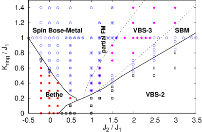
Figure 2: (Color online) Phase diagram of the ring model Eq. (1) determined in the DMRG using system sizes $L=48-96$. Filled squares (red) denote Bethe-chain phase. Open squares (with black outlines) denote Valence Bond Solid with period 2. Open circles (blue) denote Spin Bose-Metal. Open circles with crosses denote where the DMRG has difficulties converging to singlet for the larger sizes, but where we still think this is spin-singlet SBM. Star symbols denote points where the ground state appears to have true non-zero spin (for all points here, the magnetization is smaller than full polarization of the smaller Fermi sea in the SBM interpretation). Filled diamonds (magenta) denote VBS with period 3. Our identifications are ambiguous in the lower VBS-3 region approaching VBS-2. Lines indicate phase boundaries determined in VMC using spin-singlet wavefunctions described in the text (we also used appropriate dimerized wavefunctions for the VBS states). A detailed study of a cut $K_{\rm ring}/J_{1}=1$ is presented in Sec. III (cf. Fig. 8).

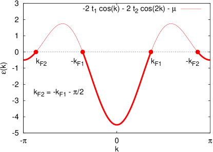
Figure 3: Spinon dispersion for $t_{2}>0.5t_{1}$ showing two occupied Fermi sea segments (here and throughout we use the 1D chain language, see bottom Fig. 1). Gutzwiller projection of this is the zigzag SBM state at the focus of this work.

A caricature of the zigzag Spin Bose-Metal is provided by considering a Gutzwiller trial wavefunction construction on the two-leg strip. The 2D SBM is obtained by letting spinons hop on the triangular lattice with no fluxes and then Gutzwiller-projecting to get a trial spin wavefunction. So here we also take spinons hopping on the ladder with no fluxes, which is $t_{1}-t_{2}$ hopping in the 1D chain language that we mainly use. For $t_{2}<0.5t_{1}$, the mean field state has one Fermi sea segment spanning $[-\pi/2,\pi/2]$ (spinons are at half-filling), and the Gutzwiller projection of this is known to be an excellent state for the Bethe chain. On the other hand, for $t_{2}>0.5t_{1}$, the spinon band has two Fermi seas as shown in Fig. 3. The Gutzwiller projection of this is a new phase that we identify as a quasi-1D descendant of the triangular lattice Spin Bose-Metal. The wavefunction has one variational parameter $t_{2}/t_{1}$, or, equivalently, the ratio of the two Fermi sea volumes. Using this restricted family of states, our VMC energetics study of the $J_{1}-J_{2}-K_{\rm ring}$ model finds three regimes broadly delineated by solid lines in Fig. 3 for larger $K_{\rm ring}$: i) In the Bethe-chain regime the optimal state has one Fermi sea. ii) For sufficiently large $K_{\rm ring}$ and upon increasing $J_{2}$, we enter a different regime where it is advantageous to start populating the second Fermi sea. As we further increase $J_{2}$ moving away from the Bethe-chain phase, we gradually transfer more spinons from the first to the second Fermi sea. This whole region is the SBM. iii) Finally, at still larger $J_{2}$, the volumes of the two Fermi seas become equal, which corresponds to $t_{2}/t_{1}\to\infty$, i.e., decoupled-legs limit.

The DMRG is the crucial tool that allows us to answer how much of this trial state picture actually holds in the $J_{1}-J_{2}-K_{\rm ring}$ model. Fig. 2 shows all points that were studied using the DMRG and their tentative phase identifications by looking at various ground state properties. Remarkably, in a broad-brush sense, the three regimes found in VMC for $K_{\rm ring}>0.2$ (one spinon Fermi sea, two generic Fermi seas, and decoupled legs) match quite closely different qualitative behaviors found by the DMRG study and marked as Bethe-chain, SBM, and VBS-2 regions. Here we note that the decoupled-legs Gutzwiller wavefunction is gapless and does not have VBS-2 order, but it is likely unstable towards opening a spin gap;White and Affleck (1996); Nersesyan et al. (1998) still, it is a good initial description for large $J_{2}$. On the other hand, away from the decoupled-legs limit, we expect a stable gapless SBM phase. The DMRG measures spin and dimer correlations, and we identify the SBM by observing singularities at characteristic wavevectors that evolve continuously as we move through this phase – these are the quasi-1D “Bose points” (remnants of a 2D Bose surface). The singular wavevectors are reproduced well by the VMC, although the Gutzwiller wavefunctions apparently cannot capture the amplitudes and power law exponents.

An effective low energy field theory for the zigzag SBM phase can be obtained by employing Bosonization to analyze either a spinon gauge theory formulation or an interacting model of electrons hopping on the zigzag chain. In the latter case we identify an Umklapp term which drives the two-band metal of interacting electrons through a Mott metal-insulator transition. The low energy Bosonized description of the Mott insulating state thereby obtained is identical to that obtained from the zigzag spinon gauge theory. In the interacting electron case, there are physical electrons that exist above the charge gap. On the other hand, in the gauge theory the “spinons” are unphysical and linearly confined.

The low energy fixed point theory for the zigzag Spin Bose-Metal phase consists of three gapless (free Boson) modes, two in the spin sector and one in the singlet sector (the latter we identify with spin chirality fluctuations). Because of the SU(2) spin invariance, there is only one Luttinger parameter in the theory, and we can characterize all power laws using this single parameter. The dominant correlations occur at wavevectors $2k_{F1}$ and $2k_{F2}$ connecting opposite Fermi points, and the power law can vary between $x^{-3/2}$ and $x^{-1}$ depending on the value of the Luttinger parameter. We understand well the stability of this phase. We also understand why the Gutzwiller-projected wavefunctions, while capturing the singular wavevectors, are not fully adequate – our trial wavefunctions appear to be described by a specific value of the Luttinger parameter that gives $x^{-3/2}$ power law at $2k_{F1}$ and $2k_{F2}$. The difference between the DMRG and VMC in the SBM phase is qualitatively captured by the low energy Bosonized theory.

The full DMRG phase diagram findings are in fact much richer. Prominently present in Fig. 2 is a new phase occurring inside the SBM and labeled VBS-3. This has period-3 Valence Bond Solid order “dimerizing” every third bond and also has coexisting effective Bethe-chain-like state formed by non-dimerized spins (see Sec. V.1 and Fig. 14 for more explanations). A careful look at the SBM theory reveals that at a special commensuration where the volume of the first Fermi sea is twice as large as that of the second Fermi sea, the SBM phase can be unstable gapping out the first Fermi sea and producing such VBS-3 state.

Another observation in Fig. 2 is the possibility of developing a partial ferromagnetic (FM) moment in the SBM region labeled “partial FM” to the left of the VBS-3 phase. We do not understand all details in this region. In the SBM further to the left, we think the ground state is spin-singlet, which is what we find from the DMRG for smaller system sizes up to $L=48$. However, the DMRG already has difficulties converging to the spin-singlet state for the larger system sizes $L\sim 96$. In the partial FM region, it seems that the ground state has a small magnetization. Given our SBM picture, it is conceivable that one or both spinon Fermi seas could develop some spin polarization. The most likely scenario is for the polarization to first appear in the smaller Fermi sea since it is more narrow in energy (more flat-band-like). The total spin that we measure in the partial FM region in Fig. 2 is smaller than what would be expected from a full polarization of the second Fermi sea, and it is hard for us to analyze such states.

To check our intuition, we have also considered a modified model with an additional third-neighbor coupling $J_{3}$ which can be either antiferromagnetic or ferromagnetic tailored to either suppress the ferromagnetic tendencies or to reveal them more fully. We have studied this model at $K_{\rm ring}=J_{1}=1$, varying $J_{2}$. With antiferromagnetic $J_{3}=0.5$, we have indeed increased the stability of spin-singlet states in the region to the left of the VBS-3. Interestingly, this study, which is not polluted by the small moment difficulties, also revealed a new spin-gapped phase near the VBS-3. The new phase has a particular period-4 order in the spin chirality, and we can understand the occurrence as an instability at another commensuration point hit by the singular wavevectors as they vary in the SBM phase (see Sec. IV.5 for details). Turning now to ferromagnetic $J_{3}=-0.5$, we have found a more clear example of the partial ferromagnetism where the ground state is well described by Gutzwiller-projecting a state with a fully polarized second Fermi sea and an unpolarized first Fermi sea.

The paper is organized as follows. To set the stage, in Sec. II we develop general theory of the zigzag SBM phase. In Sec. III we present the DMRG study of the ring model that leads to the phase diagram Fig. 2. We consider carefully the cut at $K_{\rm ring}=J_{1}$ and provide detailed characterization of the new SBM phase. In Sec. IV we study analytically the stability of the SBM. We also consider possible phases that can arise as some instabilities of the SBM. This is done in particular to address the DMRG findings of the VBS-3 and Chirality-4 states, which we present in Sec. V. To clarify the regime to the left of the VBS-3 where the DMRG runs into convergence difficulties or small moment development, we also perturb the model with antiferromagnetic (Sec. V.2) or ferromagnetic (Sec. VI) third-neighbor interaction $J_{3}$ and discuss partially polarized SBM. Finally, in Sec. VII we briefly summarize and suggest some future directions one might explore. In Appendix A, within our effective field theory analysis, we summarize the bosonization expressions for physical observables that are measured in the DMRG and VMC. In Appendix B we provide details of the Gutzwiller wavefunctions that are used throughout in the VMC analysis. In Appendix C we summarize the DMRG results for the conventional Bethe-chain and VBS-2 phases.

II Spin Bose-Metal theory on the zigzag strip

Since a wavefunction does not constitute a theory, and can at best capture a caricature of the putative SBM phase, it is highly desirable to have a field-theoretic approach. The goal here is to obtain an effective low energy theory for the SBM on the zigzag chain. In 2D the usual approach is to decompose the spin operators in terms of an SU(2) spinor – the fermionic spinons:

$$\vec{S}=\frac{1}{2}f_{\alpha}^{\dagger}\vec{\sigma}_{\alpha\beta}f_{\beta}~{};\quad\quad f_{\alpha}^{\dagger}f_{\alpha}=1~{}.$$ (2)

In the mean field one assumes that the spinons do not interact with one another and are hopping freely on the 2D lattice. For the present problem the mean field Hamiltonian would have the spinons hopping in zero magnetic field, and the ground state would correspond to filling up a spinon Fermi sea. In doing this one has artificially enlarged the Hilbert space, since the spinon hopping Hamiltonian allows for unoccupied and doubly-occupied sites, which have no meaning in terms of the spin model of interest. It is thus necessary to project back down into the physical Hilbert space for the spin model, restricting the spinons to single occupancy. If one is only interested in constructing a variational wavefunction, this can be readily achieved by the Gutzwiller projection, where one simply drops all terms in the wavefunction with unoccupied or doubly-occupied sites. The alternate approach to implement the single occupancy constraint is by introducing a gauge field, a $U(1)$ gauge field in this instance, that is minimally coupled to the spinons in the hopping Hamiltonian. This then becomes an intrinsically strongly-coupled lattice gauge field theory. To proceed, it is necessary to resort to an approximation by assuming that the gauge field fluctuations are (in some sense) weak. In 2D one then analyzes the problem of a Fermi sea of spinons coupled to a weakly fluctuating gauge field. This problem has a long history,Ioffe and Larkin (1989); Holstein et al. (1973); Reizer (1989); Lee (1989); Lee and Nagaosa (1992); Polchinski (1994); Altshuler et al. (1994); Kim et al. (1994); Lee et al. (2006) but all the authors have chosen to sum the same class of diagrams. Within this (uncontrolled) approximation one can then compute physical spin correlation functions, which are gauge invariant. It is unclear, however, whether this is theoretically legitimate, and even less clear whether or not the spin liquid phase thereby constructed captures correctly the universal properties of a physical spin liquid that can (or does) occur for some spin Hamiltonian.

Fortunately, on the zigzag chain we are in much better shape. Here it is possible to employ Bosonization to analyze the quasi-1D gauge theory, as we detail below. While this still does not give an exact solution for the ground state of any spin Hamiltonian, with regard to capturing universal low energy properties it is controlled. As we will see, the low energy effective theory for the SBM phase is a Gaussian field theory, and perturbations about this can be analyzed in a systematic fashion to check for stability of the SBM and possible instabilities into other phases.

As we will also briefly show, the low energy effective theory for the SBM can be obtained just as readily by starting with a model of interacting electrons hopping on the zigzag chain, i.e. a Hubbard-type Hamiltonian. If one starts with interacting electrons, it is (in principle) possible to construct the gapped electron excitations in the SBM Mott insulator. Within the gauge theory approach, the analogous gapped spinon excitations are unphysical, being confined together with a linear potential. Moreover, within the electron formulation one can access the metallic phase, and also the Mott transition to the SBM insulator.

II.1 SBM via Bosonization of gauge theory

We first start by using BosonizationShankar (1995); Lin et al. (1998); Fjaerestad and Marston (2002) to analyze the gauge theory.Kim and Lee (1999); Hosotani (1997); Mudry and Fradkin (1994) Motivated by the 2D triangular lattice with ring exchanges, we assume a mean field state in which the spinons are hopping in zero flux. Here the spinons are hopping on the zigzag strip with near-neighbor and second-neighbor hopping strengths denoted $t_{1}$ and $t_{2}$. This is equivalent to a strictly 1D chain with likewise first- and second-neighbor hopping. The dispersion is

$$\xi(k)=-2t_{1}\cos(k)-2t_{2}\cos(2k)-\mu~{}.$$ (3)

For $t_{2}>0.5t_{1}$ there are two sets of Fermi crossings at wave vectors $\pm k_{F1}$ and $\pm k_{F2}$ as shown in Fig. 3. Our convention is that fermions near $k_{F1}$ and $k_{F2}$ are moving to the right; the corresponding group velocities are $v_{1},v_{2}>0$. The spinons are at half-filling, which implies $k_{F1}+k_{F2}=-\pi/2\mod 2\pi$.

The spinon operators are expanded in terms of continuum fields,

$$f_{\alpha}(x)=\sum_{a,P}e^{iPk_{Fa}x}f_{Pa\alpha}~{},$$ (4)

with $a=1,2$ denoting the two Fermi seas, $\alpha=\uparrow,\downarrow$ denoting the spin, and $P=R/L=\pm$ denoting the right and left moving fermions. We now use Bosonization,Shankar (1995); Lin et al. (1998); Fjaerestad and Marston (2002) re-expressing these low energy spinon operators with Bosonic fields,

$$f_{Pa\alpha}=\eta_{a\alpha}e^{i(\varphi_{a\alpha}+P\theta_{a\alpha})}~{},$$ (5)

with canonically conjugate boson fields:

$$[\varphi_{a\alpha}(x),\varphi_{b\beta}(x^{\prime})] = [\theta_{a\alpha}(x),\theta_{b\beta}(x^{\prime})]=0~{},$$ (6)

$$~{}[\varphi_{a\alpha}(x),\theta_{b\beta}(x^{\prime})] = i\pi\delta_{ab}\delta_{\alpha\beta}\,\Theta(x-x^{\prime})~{},$$ (7)

where $\Theta(x)$ is the Heaviside step function. Here, we have introduced Klein factors, the Majorana fermions $\{\eta_{a\alpha},\eta_{b\beta}\}=2\delta_{ab}\delta_{\alpha\beta}$, which assure that the spinon fields with different flavors anti-commute with one another. The (slowly varying) fermionic densities are simply $f_{Pa\alpha}^{\dagger}f_{Pa\alpha}=\partial_{x}(P\varphi_{a\alpha}+\theta_{a\alpha})/(2\pi)$.

A faithful formulation of the physical system in this slave particle approach Eq. (2) is a compact U(1) lattice gauge theory. In 1+1D continuum theory, we work in the gauge eliminating spatial components of the gauge field. The imaginary-time bosonized Lagrangian density is then:

$${\cal L}=\frac{1}{2\pi}\sum_{a\alpha}\left[\frac{1}{v_{a}}(\partial_{\tau}\theta_{a\alpha})^{2}+v_{a}(\partial_{x}\theta_{a\alpha})^{2}\right]+{\cal L}_{A}~{}.$$ (8)

Here ${\cal L}_{A}$ encodes the coupling to the slowly varying 1D (scalar) potential field $A(x)$,

$${\cal L}_{A}=\frac{1}{m}(\partial_{x}A/\pi)^{2}+i\rho_{A}A~{},$$ (9)

where $\rho_{A}$ denotes the total “gauge charge” density,

$$\rho_{A}=\sum_{a\alpha}\partial_{x}\theta_{a\alpha}/\pi~{}.$$ (10)

It is useful to define “charge” and “spin” boson fields,

$$\theta_{a\rho/\sigma}=\frac{1}{\sqrt{2}}(\theta_{a\uparrow}\pm\theta_{a\downarrow})~{},$$ (11)

and “even” and “odd” flavor combinations,

$$\theta_{\mu\pm}=\frac{1}{\sqrt{2}}(\theta_{1\mu}\pm\theta_{2\mu})~{},$$ (12)

with $\mu=\rho,\sigma$. Similar definitions hold for the $\varphi$ fields. The commutation relations for the new $\theta,\varphi$ fields are unchanged.

Integration over the gauge potential generates a mass term,

$${\cal L}_{A}=m(\theta_{\rho+}-\theta_{\rho+}^{(0)})^{2}~{},$$ (13)

for the field $\theta_{\rho+}=\sum_{a\alpha}\theta_{a\alpha}/2$. In the gauge theory analysis, we cannot determine the mean value $\theta_{\rho+}^{(0)}$, which is important for detailed properties of the SBM in Appendix A as well as for the discussion of nearby phases in Secs. IV.2-IV.5. But if we start with an interacting electron model, one can readily argue that the correct value in the SBM phase satisfies

$$4\theta_{\rho+}^{(0)}=\pi\mod 2\pi~{}.$$ (14)

II.2 SBM by Bosonizing interacting electrons

Consider then a model of electrons hopping on the zigzag strip. We assume that the electron hopping Hamiltonian is identical to the spinon mean field Hamiltonian, with first and second neighbor hopping strengths, $t_{1},t_{2}$;

$$H\! = \!-\sum_{x}[t_{1}c^{\dagger}_{\alpha}(x)c_{\alpha}(x+1)+t_{2}c^{\dagger}_{\alpha}(x)c_{\alpha}(x+2)+{\rm H.c.}]$$ (15)

$$+H_{int}~{}.$$

The electrons are taken to be at half-filling. The interactions between the electrons could be taken as a Hubbard repulsion, perhaps augmented with further neighbor interactions, but we do not need to specify the precise form for what follows.

For $t_{2}<0.5t_{1}$, the electron Fermi sea has only one segment spanning $[-\pi/2,\pi/2]$, and at low energy the model is essentially the same as the 1D Hubbard model. We know that in this case even an arbitrary weak repulsive interaction will induce an allowed four-fermion Umklapp term that will be marginally relevant driving the system into a 1D Mott insulator. The residual spin sector will be described in terms of the Heisenberg chain, and is expected to be in the gapless Bethe-chain phase.

On the other hand, for $t_{2}>0.5t_{1}$, the electron band has two Fermi seas as shown in Fig. 3. This is the case of primary interest to us. As in the one-band case, Umklapp terms are required to drive the system into a Mott insulator. But in this two-band case there are no allowed four-fermion Umklapp terms. While it is possible to study perturbatively the effects of the momentum conserving four-fermion interactions and address whether or not the two-band metal is stable for some particular form of the lattice Coulomb repulsion, we do not pursue this here. Rather, we focus on the allowed eight-Fermion Umklapp term which takes the form,

$$H_{8}=v_{8}(c_{R1\uparrow}^{\dagger}c_{R1\downarrow}^{\dagger}c_{R2\uparrow}^{\dagger}c_{R2\downarrow}^{\dagger}c_{L1\uparrow}c_{L1\downarrow}c_{L2\uparrow}c_{L2\downarrow}+{\rm H.c.})~{},$$ (16)

where we have introduced slowly varying electron fields for the two bands, at the right and left Fermi points. For repulsive electron interactions we have $v_{8}>0$. This Umklapp term is strongly irrelevant at weak coupling since its scaling dimension is $\Delta_{8}=4$ (each electron field has scaling dimension $1/2$), much larger than the space-time dimension $D=2$.

To make progress we can Bosonize the electrons, just as we did for the spinons, $c_{Pa\alpha}\sim e^{i(\varphi_{a\alpha}+P\theta_{a\alpha})}$. The eight-Fermion Umklapp term becomes,

$$H_{8}=2v_{8}\cos(4\theta_{\rho+})~{},$$ (17)

where as before $\theta_{\rho+}=\sum_{a\alpha}\theta_{a\alpha}/2$ and $\rho_{e}(x)=2\partial_{x}\theta_{\rho+}/\pi$ is now the physical slowly varying electron density. The Bosonized form of the non-interacting electron Hamiltonian is precisely the first part of Eq. (8), and one can readily confirm that $\Delta_{8}=4$. But now imagine adding a strong density-density repulsion between the electrons. The slowly varying contributions, on scales somewhat larger than the lattice spacing, will take the simple form, $H_{\rho}\sim V_{\rho}\rho_{e}^{2}(x)\sim V_{\rho}(\partial_{x}\theta_{\rho+})^{2}$. These forward scattering interactions will “stiffen” the $\theta_{\rho+}$ field and will reduce the scaling dimension $\Delta_{8}$. If $\Delta_{8}$ drops below $2$ then the Umklapp term becomes relevant and will grow at long scales. This destabilizes the two-band metallic state, driving a Mott metal-insulator transition. The $\theta_{\rho+}$ field gets pinned in the minima of the $H_{8}$ potential, which gives Eq. (14). Expanding to quadratic order about the minimum gives a mass term of the form Eq. (13). For the low energy spin physics of primary interest this shows the equivalence between the direct Bosonization of the electron model and the spinon gauge theory approach.

The difference between the spinon gauge theory and the interacting electron theory are manifest in the charge sector. In the latter case the electron excitations $c^{\dagger}$ above the gap will correspond to instantons connecting adjacent minima of the cosine potential Eq. (17). In the spinon gauge theory there are no such fermionic excitations $f^{\dagger}$, and the spinon excitations are linearly confined. This is appropriate for the spin model which has no “charge sector”, and no notion of spinons. In the weak Mott insulating phase of the electron model, the Fermi wavevectors $k_{F1},k_{F2}$ denote the momenta of the minimum energy gapped electron excitations. What is the meaning, then, of the spinon Fermi wavevectors if the spinon excitations are unphysical? Within the spinon gauge theory the only gauge invariant (i.e. physical) momenta are the sums and differences of $k_{F1},k_{F2}$, which correspond to momenta of the (low energy) spin excitations. In the electron model, the spin excitations below the charge localization length of the Mott insulator will be similar to that of electrons in the metal. On longer scales, the spin sector remains gapless, and this is the regime described below by the low energy effective theory of the SBM Mott insulator. It is these physical longer length scale spin excitations which are correctly captured by both the spinon gauge theory and interacting electron approaches.

II.3 Fixed point theory of the SBM phase

The low energy spin physics in either formulation can be obtained by integrating out the massive $\theta_{\rho+}$ field, as we now demonstrate. Performing this Gaussian integration leads to the effective fixed-point (quadratic) Lagrangian for the SBM spin liquid:

$${\cal L}_{0}^{\rm SBM}={\cal L}_{0}^{\rho}+{\cal L}_{0}^{\sigma}~{},$$ (18)

with the “charge” sector contribution,

$${\cal L}_{0}^{\rho}=\frac{1}{2\pi g_{0}}\left[\frac{1}{v_{0}}(\partial_{\tau}\theta_{\rho-})^{2}+v_{0}(\partial_{x}\theta_{\rho-})^{2}\right]~{},$$ (19)

and the spin sector contribution,

$${\cal L}_{0}^{\sigma}=\frac{1}{2\pi}\sum_{a}\left[\frac{1}{v_{a}}(\partial_{\tau}\theta_{a\sigma})^{2}+v_{a}(\partial_{x}\theta_{a\sigma})^{2}\right]~{}.$$ (20)

The velocity $v_{0}$ in the “charge” sector depends on the product of the flavor velocities, $v_{0}=\sqrt{v_{1}v_{2}}$, while the dimensionless “conductance” depends on their ratio:

$$g_{0}=\frac{2}{\sqrt{v_{1}/v_{2}}+\sqrt{v_{2}/v_{1}}}~{}.$$ (21)

Notice that $g_{0}\leq 1$, with $g_{0}\to 0$ upon approaching the limit of a single Fermi surface ($v_{1}\neq 0$, $v_{2}\to 0$), and $g_{0}\to 1$ in the limit of two equally-sized Fermi surfaces ($v_{2}/v_{1}\to 1$) that occurs when the two legs of the triangular strip decouple.

In Sec. IV.1, we also consider all symmetry allowed residual short-range interactions between the low energy degrees of freedom and conclude that the above fixed-point theory can indeed describe a stable phase, with the only modification that $g_{0}\to g$ is now a general Luttinger parameter. Stability requires $g<1$. There are also three marginal interactions that need to have appropriate signs to be marginally irrelevant.

The gapless excitations in the SBM lead to power law correlations in various physical quantities at wavevectors connecting the Fermi points. Here and in the numerical study Sec. III, we focus on the following observables: spin $\vec{S}(x)$, bond energy ${\cal B}(x)$ (i.e., VBS order parameter), and spin chirality $\chi(x)$:

$${\cal B}(x) = \vec{S}(x)\cdot\vec{S}(x+1)~{},$$ (22)

$$\chi(x) = \vec{S}(x-1)\cdot[\vec{S}(x)\times\vec{S}(x+1)]~{}.$$ (23)

In Appendix A, we give detailed expressions in the continuum theory. The most straightforward contributions are obtained by writing out, e.g., $\vec{S}(x)\sim f^{\dagger}(x)\vec{\sigma}f(x)$ in terms of the continuum fermion fields and then bosonizing [see also Eqs. (72) and (74) for ${\cal B}(x)$ and $\chi(x)$]. We expect dominant power laws at wavevectors $\pm 2k_{Fa}$ and $\pm\pi/2=\mp(k_{F1}+k_{F2})$, originating from fermion bilinears composed of a particle and a hole moving in opposite directions. Such bilinears become enhanced upon projecting down into the spin sector (i.e. upon integrating out the massive $\theta_{\rho+}$ in the Bosonized field theory), and it is possible to compute the scaling dimension of any operator in terms of the single Luttinger parameter, $g$. It is also important to consider more general contributions, e.g., containing four fermion fields; this is best done using symmetry arguments and the corresponding expressions can be found in Appendix A.

Table 1 summarizes such analysis of the observables by listing scaling dimensions at various wavevectors. We describe power law correlation of a given operator $A$ at a wavevector $Q$ by specifying the scaling dimension $\Delta_{A_{Q}}$ defined from the real-space decay

$$\langle A(x)A(0)\rangle\sim\sum_{Q}\frac{e^{iQx}}{|x|^{2\Delta_{A_{Q}}}}~{}.$$ (24)

The corresponding static structure factor (i.e. Fourier transform) has momentum-space singularity $\sim|q-Q|^{2\Delta_{A_{Q}}-1}$.

	$Q=\,0$	$\pm 2k_{F1}$;	$\pm\pi/2$	$\pm(k_{F2}-k_{F1})$;	$\pi$	$\pm 4k_{F1}$
		$\pm 2k_{F2}$		$\pm(3k_{F1}+k_{F2})$
$\vec{S}$	$1$	$\frac{1}{2}+\frac{g}{4}$	$\frac{1}{2}+\frac{1}{4g}$	$\frac{1}{2}+\frac{1}{4g}+\frac{g}{4}$	1	subd.
$\cal B$					1	$g$
$\chi$		subd.			$1/g$	subd.

Table 1: Spin Bose-Metal fixed-point theory: Scaling dimensions of the spin $\vec{S}$, bond energy $\cal B$, and chirality $\chi$ observables at various wavevectors $Q$ in the top row. Entries with subdominant power laws are listed as “subd.”.

The $Q=0$ entries in Table 1 come from simple identifications

$$S^{z}_{Q=0} \sim \partial_{x}\theta_{1\sigma}+\partial_{x}\theta_{2\sigma}~{},$$ (25)

$${\cal B}_{Q=0} \sim \partial_{x}\theta_{\rho-}~{},$$ (26)

$$\chi_{Q=0} \sim \partial_{x}\varphi_{\rho-}~{}.$$ (27)

In particular, the last line provides physical meaning to the “$\rho-$” sector – this spin-singlet sector encodes low energy fluctuations of the chirality. A direct way to observe the propagating $\rho-$ mode would be to measure the spectral function of the chirality, while in the present DMRG study we detect it by a $|q|$ (i.e., V-shaped) behavior in the static structure factor at small wavevector $q$.

III DMRG study of the Spin Bose-Metal in the $J_{1}-J_{2}-K_{\rm ring}$ model on the zigzag chain

We study the ring model Eq. (1) on the two-leg triangular strip shown in Fig. 1. We use the 1D chain picture and take site labels $x=1,\dots,L$ where $L$ is the length of the system. We use exact diagonalization (ED) and density matrix renormalization group (DMRG)White (1992, 1993); Schollwock (2005) methods supplemented with variational Monte Carlo (VMC)Ceperley et al. (1977); Gros (1989) to determine the nature of the ground state of the Hamiltonian Eq. (1).

III.1 Measurement details

We first describe numerical measurements. All calculations use periodic boundary conditions in the $\hat{x}$ direction. In the ED, we can characterize states by a momentum quantum number $k$. On the other hand, our DMRG calculations are done with real-valued wavefunctions. This gives no ambiguity when the ground state carries momentum $0$ or $\pi$ and is unique. However, if the ground state carries nontrivial momentum $k\neq 0,\pi$, then its time-reversed partner carries $-k$, and the DMRG state is some combination of these. While the real space measurements depend on the specific combination in the finite system, the momentum space measurements described below do not depend on this and are unique. Most of the calculations are done in the sector with $S^{z}_{\rm tot}=0$, which contains any ground state of the SU(2)-invariant system.

The DMRG calculations keep more than $m=3200$ states per block White (1992, 1993); Schollwock (2005) to ensure accurate results, and the density matrix truncation error is of the order of $10^{-6}$. Typical relative error for the ground-state energy is of the order of $10^{-4}$ or smaller for the systems we have studied. Using ED, we have confirmed that all DMRG results are numerically exact when the system size is $L=24$. The DMRG convergence depends strongly on the phase being studied, the system size, the type of the correlations, and the distance between operators. In the Bethe-chain and VBS-2 phases there is still good convergence for size $L=192$, while in the SBM we are limited to $L=96-144$ systems. The entanglement entropy calculations are done with up to $m=6000$ states in each block, which is necessary for capturing the long range entanglement in the SBM states where we find an effective “central charge” $c\simeq 3$.

We have already specified the main observables in Sec. II.3 [cf. Eqs. (22-23)]. We measure spin correlations, bond energy (dimer) correlations, and chirality correlations defined as follows:

$$C(x,x^{\prime}) = \langle\vec{S}(x)\cdot\vec{S}(x^{\prime})\rangle~{},$$ (28)

$$D(x,x^{\prime}) = \langle{\cal B}(x){\cal B}(x^{\prime})\rangle-{\langle{\cal B}\rangle}^{2}~{},$$ (29)

$$X(x,x^{\prime}) = \langle\chi(x)\chi(x^{\prime})\rangle~{}.$$ (30)

For simplicity, we set $D(x,x^{\prime})=0$ if bonds ${\cal B}(x)$ and ${\cal B}(x^{\prime})$ have common sites, and similarly for $X(x,x^{\prime})$. Structure factors $C(q)$, $D(q)$, and $X(q)$ are obtained through Fourier transformation:

$$O(q)=\frac{1}{L}\sum_{x,x^{\prime}}O(x,x^{\prime})e^{-iq(x-x^{\prime})}~{},$$ (31)

where $O=C,D,X$. We have $O(q)=O(-q)$ and usually show only $0\leq q\leq\pi$. The spin structure factor at $q=0$ gives the total spin in the ground state:

$$C(q=0)=\frac{\langle\vec{S}_{\rm tot}^{2}\rangle}{L}=\frac{S_{\rm tot}(S_{\rm tot}+1)}{L}~{}.$$ (32)

In all figures, we loosely use “$\langle{\cal B}_{q}{\cal B}_{-q}\rangle$” and “$\langle\chi_{q}\chi_{-q}\rangle$” to denote $D(q)$ and $X(q)$ respectively.

Turning to the VMC calculations, the trial wavefunctions are described in broad terms in Sec. I and in more detail in Appendix B. The states are labeled by occupation numbers of the two Fermi seas, $(N_{1},N_{2})$. Since $N_{1}+N_{2}=L/2$, there is only one variational parameter. There are three distinct regimes: i) $N_{1}=L/2$, $N_{2}=0$, i.e., a single Fermi sea, which is appropriate for the Bethe-chain phase; ii) $N_{1}\neq N_{2}\neq 0$ appropriate for the SBM; and iii) $N_{1}=N_{2}=L/4$, i.e., decoupled legs, which is a reasonable starting point for the large $J_{2}$ limit.

In Appendix B, we describe correlations in the generic SBM wavefunctions and identify characteristic wavevectors $2k_{Fa}=2\pi N_{a}/L$, $a=1,2$, and also $\pi/2$ (see Sec. II and Table 1). One observation is that such wavefunctions correspond to a special case $g=1$ in the SBM theory and thus cannot capture general exponents. Despite this shortcoming, the wavefunctions capture the locations of the singular wavevectors observed in the DMRG. We also try to improve the wavefunctions by using a “gapless superconductor” modification described in Appendix B.2 and designed to preserve the singular wavevectors while allowing more variational parameters. This indeed improves the trial energy and provides better match with the DMRG correlations at short scales, even if the long distance properties are still not captured fully. When presenting the DMRG structure factors, we also show the corresponding VMC results for wavefunctions determined by minimizing the trial energy over the described family of states.

Using the DMRG, we find four distinct quantum phases in the $J_{2}/J_{1}-K_{\rm ring}/J_{1}$ plane as illustrated in Fig. 2. In the small $K_{\rm ring}$ region, we have the conventional Bethe-chain phase at small $J_{2}$ and Valence Bond Solid state with period 2 (VBS-2) at larger $J_{2}$. The SBM phase emerges in the regime $K_{\rm ring}>0.2J_{1}$ and dominates the intermediate parameter space. Inside this region, we discover a new VBS state with period 3 (VBS-3). To fully understand the VBS-3 (in particular, its relationship to the flanking Spin Bose-Metals) we will need the stability analysis of the SBM in Sec. IV, while the DMRG results are discussed afterwards in Sec. V.

We explore more finely a cut $K_{\rm ring}=J_{1}$ through the phase diagram Fig. 2, and our presentation points are taken from this cut. The Bethe-chain and VBS-2 phases are fairly conventional (for this $K_{\rm ring}$, the VBS-2 is close to the decoupled-legs state at large $J_{2}$ values). Nevertheless, it is useful to see measurements in these phases for comparisons. Such examples are given in Appendix C, while here we focus on the Spin Bose-Metal point deep in the phase. We will discuss more difficult parts of the phase diagram Fig. 2 once we have the overall picture of the SBM.

III.2 Representative Spin Bose-Metal points

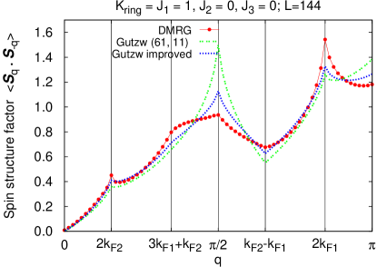
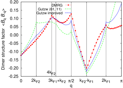
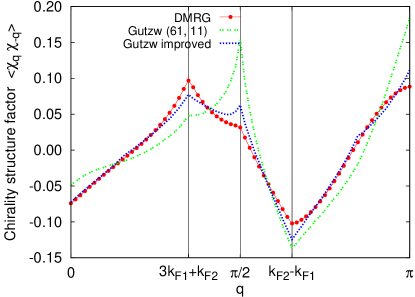
Figure 4: (Color online) Spin, dimer, and chirality structure factors at a representative point in the Spin Bose-Metal phase, $K_{\rm ring}=J_{1}=1$, $J_{2}=0$ (close to the Bethe-chain phase), measured in the DMRG for system size $L=144$. We also show the structure factors in the Gutzwiller projection of two Fermi seas $(N_{1},N_{2})=(61,11)$, and in the improved Gutzwiller wavefunction with parameters $f_{0}=1,f_{1}=0.65,f_{2}=-0.5$ (see Appendix B; the parameters are determined by optimizing the trial energy within the given family of states). Vertical lines label important wavevectors expected in the SBM theory for such spinon Fermi sea volumes. We discuss the comparison of the DMRG, VMC, and analytical theory in the text.

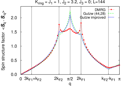
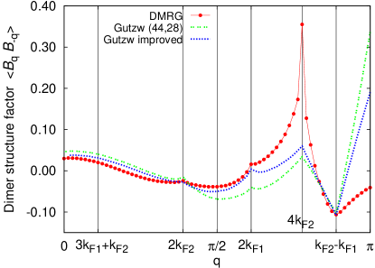
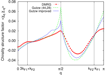
Figure 5: (Color online) Spin, dimer, and chirality structure factors at a representative point in the Spin Bose-Metal phase, $K_{\rm ring}=J_{1}=1$, $J_{2}=3.2$ (between the VBS-3 and VBS-2 phases) measured in the DMRG for system size $L=144$. We also show results in the Gutzwiller projection of two Fermi seas $(N_{1},N_{2})=(44,28)$, and in the improved Gutzwiller wavefunction with parameters $f_{0}=1,f_{1}=0.75,f_{2}=-0.1$ (see Appendix B for details). Vertical lines label important wavevectors expected in the SBM theory. We discuss the comparison of the DMRG, VMC, and analytical theory in the text.

Proceeding along the $K_{\rm ring}=J_{1}=1$ cut through Fig. 2, we start in the Bethe-chain phase at large negative $J_{2}$ (a representative point is discussed in Appendix C.1). As we change $J_{2}$ towards positive value, the system undergoes a transition at $J_{2}=-0.6$. The new phase has characteristic spin correlations that are markedly different from the Bethe-chain phase. Figure 4 shows a representative point $J_{2}=0$. The DMRG calculations are more difficult to converge and are done for smaller size $L=144$ than in the Bethe-chain phase example (see also the entanglement entropy discussion below).

Comparing with the Bethe-chain state (e.g., Fig. 22 in Appendix C.1), there is no $q=\pi$ dominance in the spin structure factor. Instead, we see three singular wavevectors located at $11\times 2\pi/144$, $\pi/2$, and $61\times 2\pi/144$. Our Gutzwiller wavefunctions determined from the energetics have $(N_{1},N_{2})=(61,11)$, and the corresponding $2k_{F2}$, $-k_{F2}-k_{F1}=\pi/2\mod 2\pi$, and $2k_{F1}$ match precisely the DMRG singular wavevectors. The improved Gutzwiller wavefunction reproduces crude short-distance features better, but it has the same long-distance properties as the bare Gutzwiller. As discussed in Appendix B, our Gutzwiller wavefunctions do not capture all power laws predicted in the general analytical theory. The wavefunctions appear to have equal exponents for spin correlations at these three wavevectors, while the theory summarized in Table 1 gives stronger singularities at $2k_{F1},2k_{F2}$ and a weaker singularity at $\pi/2$. Very encouragingly, these theoretical expectations are consistent with what we find in the DMRG, where we can visibly see the difference in the behaviors at these wavevectors, particularly when we reference against the VMC results.

Similar discussion applies to the bond energy (dimer) correlations shown in the middle panel of Fig. 4. The dominant features are at $2k_{F1}$ and $\pi/2$, and we also see a peak at a wavevector identified as $4k_{F2}$, which is indeed expected from the SBM theory, cf. Table 1. The theory predicts similar singularities at $2k_{F1}$ and $2k_{F2}$, but for some reason we do not see the $2k_{F2}$ in the DMRG data, even though it is clearly present in the bare Gutzwiller. We suspect that this is caused by the narrowness in energy of the second Fermi sea when its population is low, so the amplitude of the $2k_{F2}$ bond energy feature may be much smaller. The $2k_{F2}$ can still show up in the bare Gutzwiller since, as we discuss in Appendix B, this wavefunction knows only about the Fermi sea sizes and not about the spinon energy scales like bandwidths or Fermi velocities. The improved Gutzwiller clearly tries to remedy this, although within its limitations. The $4k_{F2}$ feature is not associated solely with the second Fermi sea and is less affected by this argument; indeed, $4k_{F2}=-4k_{F1}$, and both Fermi seas “participate” in producing this feature as can be seen from Eq. (97).

Turning to the chirality structure factor in the bottom panel of Fig. 4, we see a feature at $\pi/2$, which in the SBM theory is expected to have the same singularity as the spin and dimer at this wavevector. We also see features at wavevectors $k_{F2}-k_{F1}$ and $3k_{F1}+k_{F2}$ in all our observables; these features are expected to be $\sim|\delta q|$ (i.e., V-shaped) in the Gutzwiller wavefunctions but have weaker singularity in the SBM theory, which is reasonably consistent with the DMRG measurements. Very notable in the chirality structure factor is a $\sim|q|$ shape at small $q$. This can be viewed as a direct evidence for the gapless “$\rho-$” mode in the SBM, cf. Eq. (27). On the other hand, a feature at $\pi$ is weaker than V-shaped, in contrast with the Gutzwiller wavefunctions but in agreement with the SBM theory expectations in Table 1.

To summarize, the correlations in the SBM phase are dramatically different from the Bethe-chain phase, and we can match all the characteristic wavevectors using the Gutzwiller wavefunctions projecting two Fermi seas. We also understand the failure of the wavefunctions to reproduce the nature of the singularities and the amplitudes, while the Bosonization theory of the SBM is consistent with all DMRG observations even when the wavefunctions fail.

With further increase of $J_{2}$, continuing along the $K_{\rm ring}=J_{1}=1$ cut through Fig. 2, the SBM phase becomes prominently unstable towards the VBS-3 phase occupying the range $1.5<J_{2}<2.5$ and described in Sec. V.1. Interestingly, as we increase $J_{2}$ still further, the SBM phase reappears with its characteristic correlations shown in Fig. 5 for a representative point $J_{2}=3.2$. Much of the SBM physics discussion that we have just done at $J_{2}=0$ carries over here, with the appropriately shifted locations of the singular wavevectors. The singularities at wavevectors $q_{\rm low}=2k_{F2}$ and $q_{\rm high}=2k_{F1}$ are now more equally developed and are detected in the spin as well as dimer structure factors. The two wavevectors are closer to $\pi/2$ and are located symmetrically in accordance with the general “sum rule” $2k_{F1}+2k_{F2}=\pi$, while the comparable strengths reflect the more similar energy bandwidths of the two Fermi seas. The apparent lack of the wavevector $\pi/2$ in the DMRG dimer structure factor is similar to that in the Gutzwiller wavefunction and is a matrix element effect for the first-neighbor bond when the sizes of the two Fermi seas approach each other. On the other hand, the strength of the $4k_{F2}$ dimer feature is very notable here; it can indeed be dominant in the SBM theory for sufficiently small Luttinger parameter $g$, cf. Table 1. The improved Gutzwiller wavefunction modifies the structure factors in the right direction but clearly does not succeed reproducing them accurately – as noted before, our wavefunctions do not contain the full physics expected in the Bosonized theory.

One technical remark that we want to make here is that the DMRG ground state at this point $J_{2}=3.2$ and size $L=144$ appears to have non-trivial momentum quantum number $k\neq 0,\pi$. We deduce this by observing that the measured correlations $O(x,x^{\prime})$ depend not just on $x-x^{\prime}$ but on both $x$ and $x^{\prime}$, and by seeing characteristic beatings as a function of $x$ and $x^{\prime}$ (while the $q$-space structure factors are well-converged). On the other hand, the VMC wavefunction shown in Fig. 5 has momentum zero (see Appendix B) and all measurements depend on $x-x^{\prime}$ only. If we assume that the beatings originate from the DMRG state being a superposition of $|k\rangle$ and $|-k\rangle$, we can extract $2k$ and find it to be consistent with the state $|k\rangle$ constructed from the VMC by moving one spinon across one of the Fermi seas ($2k=4k_{F2}=-4k_{F1}$). It is plausible that such state happens to have a slightly lower energy in the given finite system (e.g., at the same $J_{2}=3.2$, we find trivial $k$ for $L=72$ but non-trivial $k$ for $L=96$, likely reflecting finite-size effects on the filling of the last few spinon orbitals). We have not attempted to construct a trial spin-singlet state with the right momentum quantum number for the present $L$. Still, we expect that the structure factors are not very sensitive to such rearrangements of few spinons in the large system limit. Indeed, we find that the structure factors have the same features for different system lengths $L=72$, $96$, and $144$. It is also worth repeating that our structure factor measurements using Eq. (31) do not depend on which specific combination of $|k\rangle$ and $|-k\rangle$ is found by the DMRG procedure.

III.3 Evolution of the singular wavevectors in the SBM

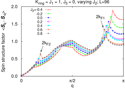
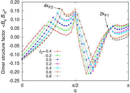
Figure 6: (Color online) Evolution of the structure factors in the Spin Bose-Metal phase between the Bethe-chain and VBS-3 (or partial FM), measured by the DMRG for system size $L=96$. We can track singular wavevectors (“Bose surfaces”) as spinons are transfered from the first to the second Fermi sea upon increasing $J_{2}$. In the spin structure factor, the wavevector $q_{\rm high}$ that starts near $\pi$ is identified as $2k_{F1}$ and the wavevector $q_{\rm low}$ that starts near $0$ is identified as $2k_{F2}$ (see Fig. 4 and text for details). The $q_{\rm high}$ and $q_{\rm low}$ are summarized in Fig. 8.

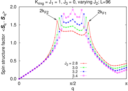
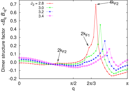
Figure 7: (Color online) Evolution of the structure factors in the Spin Bose-Metal phase between VBS-3 and VBS-2, measured by the DMRG for system size $L=96$. The $q_{\rm high}=2k_{F1}$ and $q_{\rm low}=2k_{F2}$ bracket the $\pi/2$ and approach each other with increasing $J_{2}$ (they are summarized in Fig. 8). Very notable here is the strong $4k_{F2}$ peak in the dimer structure factors that evolves out of the Bragg peak present in the VBS-3 phase at $2\pi/3$ (see Sec. V.1 and Fig. 15); the $2k_{F1}$ moves away from the $2\pi/3$ in the opposite direction.

We further illustrate the Spin Bose-Metal by showing evolution of the DMRG structure factors and singular wavevectors as we move inside the phase. The spin and dimer structure factors are shown in Fig. 6 for $L=96$ and varying parameter $J_{2}/J_{1}$ inside the SBM phase adjacent to the Bethe-chain phase. With increasing $J_{2}$, the singular wavevector $q_{\rm high}$ (identified as $2k_{F1}$ in the VMC) is moving away from $\pi$ towards smaller values, while the singular wavevector $q_{\rm low}$ (identified as $2k_{F2}$) is moving to larger values; this corresponds to spinons being transfered from the first to the second Fermi sea as found in the VMC energetics. The spin and dimer correlations show similar behavior at $2k_{F1}$, and both have features also at the wavevector $\pi/2$. The lack of visible dimer feature at $2k_{F2}$ was discussed for the point $J_{2}=0$ earlier, and it is likely that something similar is at play here. On one hand, the second band is narrow when we just enter the SBM since the second Fermi sea starts small. On the other hand, in the region labeled “partial FM”close to the VBS-3 phase in Fig. 2, the DMRG finds nonzero magnetization in the ground state. We think that this occurs in the second Fermi sea and indicates an effective narrowness of this band near the VBS-3 phase as well, so the $2k_{F2}$ energy feature may indeed be weak in the whole SBM phase between the Bethe-chain and VBS-3.

We think that the same physics also starts causing convergence difficulties in the DMRG for the $L=96$ systems shown in Fig. 6. Specifically, we can use Eq. (32) to extract the ground state spin $S_{\rm tot}$ and find non-integer values of order 1, e.g., $S_{\rm tot}(S_{\rm tot}+1)=0.3$, $1.0$, $1.9$, $2.1$, $3.4$ for the points $J_{2}=0$, $0.2$, $0.4$, $0.6$, $0.8$ in Fig. 6. This can only happen if the DMRG is not converged and is mixing several states that are close in energy but have different spin. Correspondingly, we observe a difference between $\langle S^{z}_{q}S^{z}_{-q}\rangle$ and $\langle S^{x}_{q}S^{x}_{-q}\rangle$ structure factors (recall that we are working in the sector $S^{z}_{\rm tot}=0$). We do not show these graphs, but the difference is localized near $2k_{F2}$, where the $\langle S^{z}_{q}S^{z}_{-q}\rangle$ has much sharper feature while the $\langle S^{x}_{q}S^{x}_{-q}\rangle$ has weaker feature. On the other hand, there is essentially no difference near $2k_{F1}$. This strongly suggests that the origin of the convergence difficulties lies with the second Fermi sea. The $\langle\vec{S}_{q}\cdot\vec{S}_{-q}\rangle$ structure factor that is shown in Fig. 6 does not mix different $S_{\rm tot}$ states but only sums the corresponding structure factors and is less sensitive to these convergence issues. The fact that the peaks in the top panel of Fig. 6 are located symmetrically with respect to $\pi/2$ suggests that this region is still spin-singlet SBM (but is on the verge of some magnetism in the second band). Finally, the $S_{\rm tot}$ values for the same parameters but system size $L=48$ are indeed well converged to zero, however with increasing number of states needed in the DMRG blocks for larger $J_{2}$. We thus conclude that the points in Fig. 6 are spin-singlet SBM. The DMRG convergence difficulties for the larger $L$ are in accord with the presence of many low-energy excitations (see also the discussion of the entanglement entropy below). We will further test our intuition that this region is close to some weak subband ferromagnetism in Secs. V.2 and VI by adding antiferromagnetic or ferromagnetic $J_{3}$ to suppress or enhance the FM tendencies.

Consider now Fig. 7 that shows evolution of the structure factors in the SBM phase between the VBS-3 and VBS-2. The $q_{\rm high}=2k_{F1}$ and $q_{\rm low}=2k_{F2}$ continue moving towards each other with increasing $J_{2}$, and the spin structure factors become nearly symmetric with respect to $\pi/2$. When the $q_{\rm high}$ and $q_{\rm low}$ peaks merge at $\pi/2$, which in the VMC would correspond to decoupled legs, one expectsWhite and Affleck (1996); Nersesyan et al. (1998) that a new instability will likely emerge resulting in a VBS-2 state (we discuss a representative point in Appendix C.2).

A very notable feature in the SBM dimer structure factor is the strong $4k_{F2}$ peak. Foretelling a bit, this peak can be traced as evolving out of the dimer Bragg peak at $2\pi/3$ of the VBS-3 phase to be discussed in Sec. V.1. Turning this around and approaching the VBS-3 phase by decreasing $J_{2}$, we can view the VBS-3 as an SBM instability when the dimer $4k_{F2}$ peak merges with the $2k_{F1}$ singularity, $4k_{F2}=2k_{F1}=2\pi/3$.

Finally, in this SBM region the DMRG converges well to spin-singlet states. The remark we made when discussing the point $J_{2}=3.2$ applies to all points shown in Fig. 7 with $L=96$: they show correlations $O(x,x^{\prime})$ beating in both $x$ and $x^{\prime}$, which can be interpreted similarly to the earlier $J_{2}=3.2$ case by assuming superposition of degenerate ground states with opposite momentum quantum numbers.

Fig. 8 summarizes the singular spin wavevectors extracted from plots like Figs. 6 and 7, superimposed on the phase diagram of the model along the cut $K_{\rm ring}=J_{1}$. Remarkably, the singular wavevectors throughout the entire SBM phase are well captured by the improved Gutzwiller wavefunctions, as we have illustrated in Figs. 4 and 5. These singular wavevectors are intimately connected to the sign structure of the ground state wavefunction, indicating a striking coincidence between the exact DMRG ground state wavefunction and the Gutzwiller projected VMC wavefunction. Besides the SBM regions, Fig. 8 also shows the Bethe-chain (cf. Appendix C.1), VBS-2 (Appendix C.2), and VBS-3 (Sec. V.1) phases.

We now mention more difficult points in the overall phase diagram. The lightly hatched SBM region in Fig. 8 indicates the discussed rising DMRG difficulties of not converging to an exact singlet for $L=96$. Such DMRG states are shown as open circles with crosses in Fig. 2. As we have already mentioned, the estimated $S_{\rm tot}$ values are not converged and are of order $1$ for $L=96$ (but are converged to zero for $L=48$), while $q_{\rm low}$ and $q_{\rm high}$ are located symmetrically around $\pi/2$; all this suggests that the phase is spin-singlet SBM. On the other hand, at points $J_{2}=1.2-1.5$ not marked in Fig. 8 but shown as star symbols in Fig. 2, the estimated $S_{\rm tot}$ values are larger and the apparent dominant wavevectors are no longer located symmetrically. Here we suspect a modification of the ground state, likely towards partial polarization of the second Fermi sea; this “partial FM” region is also indicated by cross-hatching in Fig. 8.

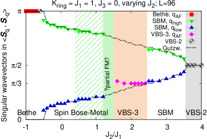
Figure 8: (Color online) Cut through the phase diagram Fig. 2 at $K_{\rm ring}/J_{1}=1$, showing evolution of the most prominent wavevectors in the spin structure factor. In the Bethe-chain phase we have singular antiferromagnetic $q_{\rm AF}=\pi$, cf. Fig. 22. In the Spin Bose-Metal we have singular $q_{\rm high}=2k_{F1}$ and $q_{\rm low}=2k_{F2}$ located symmetrically about $\pi/2$, cf. Figs. 6 and 7. In the VBS-3 we have singular $q_{\rm AF}=\pi/3$, cf. Fig. 15. In the VBS-2 region for large $J_{2}$, cf. Fig. 23, we have dominant correlations at $\pi/2$ corresponding to the decoupled legs fixed point, which is likely to be unstable towards opening a spin gap.White and Affleck (1996); Nersesyan et al. (1998) The dotted lines show results for the improved Gutzwiller wavefunction.

III.4 Entanglement entropy and effective central charge of the SBM

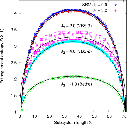
Figure 9: (Color online) Entanglement entropy at representative points in the Bethe-chain ($J_{2}=-1$), SBM ($J_{2}=0$ and $J_{2}=3.2$), VBS-3 ($J_{2}=2$), and VBS-2 ($J_{2}=4$) phases, taken from the cut $K_{\rm ring}=J_{1}=1$, measured in the DMRG for system size $L=72$ with periodic boundary conditions. We use Eq. (33) to fit data over the range $6\leq X\leq 66$, which gives the best estimates as $c=1.0$ (Bethe-chain), $c=3.1$ (SBM at $J_{2}=0$), $c=3.2$ (SBM at $J_{2}=3.2$), $c=1.6$ (VBS-3), and $c=2.1$ (VBS-2).

We explore properties of the SBM phase that can further distinguish it from the Bethe-chain and VBS states. Earlier we have noted that we need to keep more states per block to achieve similar convergence for the SBM phase in comparison with the Bethe-chain and VBS phases, indicating stronger entanglement between subsystems in the SBM. Bosonization analysis finds that the SBM fixed point theory has three free Boson modes. One can associate a central charge $1$ with each mode. Despite the fact that they have different velocities (so the full system is not conformally invariant), we expect that the total entanglement entropy should have a universal behavior described by a combined central charge $c=3$.

In general, for a one-dimensional gapless state with conformally invariant correlation functions in space-time, the entanglement entropy for a finite subsystem of length $X$ inside a system of length $L$ with periodic boundary conditions varies asCalabrese and Cardy (2004)

$$S(X,L)=\frac{c}{3}\log\left(\frac{L}{\pi}\sin\frac{\pi X}{L}\right)+A~{},$$ (33)

where $A$ is a constant (independent of the subsystem length) and $c$ is the effective central charge. The virtue of the entanglement entropy is that it does not depend on the mode velocities and in principle measures the number of gapless modes directly from the ground state wavefunction.

Figure 9 shows the entanglement entropy $S(X,L)$ as a function of $X$ for different quantum phases for a finite system length $L=72$. The results are obtained from the DMRG for representative points taken from the same cut $K_{\rm ring}=J_{1}=1$ discussed earlier. The entropy can be well fitted by the ansatz Eq. (33) with different $c$ values.

The Bethe-chain state (at $J_{2}=-1$) gives central charge $c=1.0$ consistent with one gapless mode. On the other hand, the entanglement entropy for either of the two SBM examples $J_{2}=0$ and $J_{2}=3.2$ is much larger and can be fitted by close values $c=3.1$ and $c=3.2$, respectively. The closeness of the central charges in these two different SBM states (cf. Figs. 4 and 5) indicates the universal behavior of the entanglement which is independent of the details like the relative sizes of the spinon Fermi seas.

Interestingly, the VBS-2 point at $J_{2}=4$ is fitted by $c=2.1$, which is related to the fact that the wavefunction is close to the decoupled-legs limit (see Appendix C.2 and Fig. 23), and this $L=72$ system “does not know” about the eventual spin gap and very small dimerization.

Finally, the fitted effective central charge for the VBS-3 example is around $c=1.6$. The oscillatory behavior of $S(X)$ reflects translational symmetry breaking in the DMRG state. Note that the entropy values are larger here compared with the Bethe-chain or VBS-2 cases, which is probably due to a mix of degenerate states in the DMRG wavefunction. However, the overall $X$-dependence is clearly weaker than in the VBS-2 and is approaching the Bethe-chain behavior for large $X$.

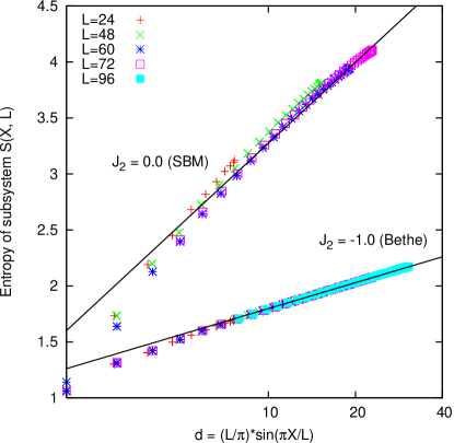
Figure 10: (Color online) Entanglement entropy for various system sizes for the Bethe-chain ($J_{2}=-1$) and SBM ($J_{2}=0$) points, cf. Fig. 9, plotted versus scaling variable $d=\frac{L}{\pi}\sin\frac{\pi X}{L}$. We also show fits to Eq. (33) done for the larger sizes. The Bethe-chain data collapses well and is fitted with $c=1$. The SBM data is fitted with $c=3.1$ (we show the same fit as in Fig. 9 for this SBM point). The collapse of different $L$ is less good, which is likely due to imprecise scaling of the discrete shell filling numbers with $L$ (see text for details).

To better understand finite size effects, we focus on the SBM and Bethe-chain phases and discuss the universal dependence of the entropy on the scaling variable $d=\frac{L}{\pi}\sin\frac{\pi X}{L}$. Figure 10 shows $S(X,L)$ as a function of $d$ for several system sizes for the SBM point $J_{2}=0$ and the Bethe-chain point $J_{2}=-1$.

At the SBM point, the data for the two larger sizes $L=60$ and $72$ collapse onto one curve, which can be reasonably fitted by $S(X,L)=(3.1/3)\log(d)+0.88$, strongly suggesting the effective central charge $c\simeq 3$. The smaller sizes $L=24$ and $48$ have somewhat shifted entropy values compared with the $L=60$ and $72$ collapse, but show roughly similar slope for the largest $d$. The differences are likely due to finite-size shell filling effects. Indeed, we can measure the structure factors and characterize the presumed SBM states by the spinon occupation numbers of the two Fermi seas; we find $(N_{1},N_{2})=(10,2)$, $(20,4)$, $(26,4)$, and $(31,5)$ for $L=24$, $48$, $60$, and $72$ respectively, and these numbers in each Fermi sea do not precisely “scale” with $L$.

On the other hand, the Bethe-chain case does not have such effects and data for all sizes collapse. The results can be well fitted by $S(X,L)=(1/3)\log(d)+0.99$ as shown in the same figure for system sizes $L=24$ to $96$. We note that while the entropy for the Bethe-chain phase for $L=96$ is fully converged by keeping up to $m=4200$ states in the DMRG block, the entropy for the SBM for $L=72$ is still increasing slowly with the number of states kept, and we estimate that the error in $S(X=L/2,L)$ is around a few percent when $m=6000$ states are kept per block (comparing to an extrapolation to $m=\infty$). Indeed, the SBM data for $L=72$ is bending down slightly from the fitted line at the larger $d$ corresponding to $X\sim L/2$, as can be seen in Fig 10, which is probably because the data is less converged.

To summarize, the entanglement entropy calculations establish the SBM as a critical phase with three gapless modes and clearly distinguish it from the Bethe-chain and VBS-2 phases (or the decoupled-legs limit). We also note that the structure factor measurements and detection of all features as in Figs. 6 and 7 did not require as much effort and was done for larger sizes than the entropy; however, to characterize the long distance power laws accurately one would probably need to capture all entanglement, which we have not attempted.

IV Stability of the Spin Bose-Metal phase; nearby phases out of the SBM

IV.1 Residual interactions and stability of the SBM

We account for residual interactions between low-energy degrees of freedom in the SBM theory, Sec. II, by considering all allowed short-range interactions of the spinons. The four-fermion interactions can be conveniently expressed in terms of chiral currents:

$$J_{Pab}=f^{\dagger}_{Pa\alpha}f_{Pb\alpha}~{};\quad\vec{J}_{Pab}=\frac{1}{2}f^{\dagger}_{Pa\alpha}\vec{\sigma}_{\alpha\beta}f_{Pb\beta}~{}.$$ (34)

We assume that interactions that are chiral, say involving only right movers, can be neglected apart from velocity renormalizations. The most general four-fermion interactions which mix right and left movers can be succinctly written as,

$${\cal L}^{\rho}_{1} = \sum_{a,b}\left(w^{\rho}_{ab}J_{Rab}J_{Lab}+\lambda^{\rho}_{ab}J_{Raa}J_{Lbb}\right)~{},$$ (35)

$${\cal L}^{\sigma}_{1} = -\sum_{a,b}\left(w^{\sigma}_{ab}\vec{J}_{Rab}\cdot\vec{J}_{Lab}+\lambda^{\sigma}_{ab}\vec{J}_{Raa}\cdot\vec{J}_{Lbb}\right)~{},$$ (36)

with $w_{11}=w_{22}=0$ (convention), $w_{12}=w_{21}$ (from Hermiticity), and $\lambda_{12}=\lambda_{21}$ (from $R\leftrightarrow L$ symmetry). There are 8 independent couplings: $w_{12}^{\rho/\sigma}$, $\lambda_{11}^{\rho/\sigma}$, $\lambda_{22}^{\rho/\sigma}$, and $\lambda_{12}^{\rho/\sigma}$.

We treat these interactions perturbatively as follows. First we bosonize the interactions and obtain terms quadratic in $\partial_{x}\theta_{a\alpha}$ and $\partial_{x}\varphi_{a\alpha}$ as well as terms involving products of four exponentials $e^{\pm i\theta_{a\alpha}}$ and $e^{\pm i\varphi_{a\alpha}}$. We next impose the condition that $\theta_{\rho+}$ is pinned and compute the scaling dimensions of the exponential operators.

The $w_{12}^{\rho/\sigma}$ terms give

$$W\equiv(w_{12}^{\rho}J_{R12}J_{L12}-w_{12}^{\sigma}\vec{J}_{R12}\cdot\vec{J}_{L12})+{\rm H.c.}=~{}~{}~{}~{}~{}~{}~{}~{}$$ (37)

$$=\cos(2\varphi_{\rho-})\Bigg{\{}4w_{12}^{\rho}\Big{[}\cos(2\varphi_{\sigma-})-\hat{\Gamma}\cos(2\theta_{\sigma-})\Big{]}~{}~{}~{}~{}~{}~{}~{}$$ (38)

$$~{}-w_{12}^{\sigma}\Big{[}\cos(2\varphi_{\sigma-})+\hat{\Gamma}\cos(2\theta_{\sigma-})+2\hat{\Gamma}\cos(2\theta_{\sigma+})\Big{]}\Bigg{\}},$$ (39)

where

$$\hat{\Gamma}=\eta_{1\uparrow}\eta_{1\downarrow}\eta_{2\uparrow}\eta_{2\downarrow}~{}.$$ (40)

The $w_{12}^{\rho/\sigma}$ terms have scaling dimension $1+g_{0}^{-1}\geq 2$ and are irrelevant in the bare theory, Eq. (18), and henceforth dropped. The detailed $W$ expression will be used later when we analyze phases neighboring the SBM.

The remaining exponentials only depend on the fields $\theta_{a\sigma}$ and $\varphi_{a\sigma}$ so that the charge and spin sectors decouple. Since the rest of ${\cal L}^{\rho}_{1}$ is quadratic, ${\cal L}^{\rho}={\cal L}^{\rho}_{0}+{\cal L}^{\rho}_{1}$ takes the same form as ${\cal L}^{\rho}_{0}$ in Eq. (19) except with $g_{0},v_{0}\to g,v$, where

$$g^{2} = 4\frac{(v_{1}-\lambda_{11}^{\rho}/\pi)(v_{2}-\lambda_{22}^{\rho}/\pi)-(\lambda_{12}^{\rho}/\pi)^{2}}{(v_{1}+v_{2}-2\lambda_{12}^{\rho}/\pi)^{2}-(\lambda_{11}^{\rho}/\pi+\lambda_{22}^{\rho}/\pi)^{2}}~{},$$ (41)

$$v = \frac{g}{2}(v_{1}+v_{2}+\lambda_{11}^{\rho}/\pi+\lambda_{22}^{\rho}/\pi-2\lambda_{12}^{\rho}/\pi)~{}.$$ (42)

In the spin sector, the remaining interactions are given by,

$$\tilde{\cal L}^{\sigma}_{1}=-\sum_{a}\lambda^{\sigma}_{aa}\vec{J}_{Raa}\cdot\vec{J}_{Laa}-\lambda^{\sigma}_{12}(\vec{J}_{R11}\cdot\vec{J}_{L22}+\vec{J}_{L11}\cdot\vec{J}_{R22})~{}.$$ (43)

When we write this in the bosonization, the $J^{z}_{R}J^{z}_{L}$ pieces contribute to the harmonic part of the action

$$V_{z} = \sum_{a}\frac{\lambda_{aa}^{\sigma}}{8\pi^{2}}\left[(\partial_{x}\varphi_{a\sigma})^{2}-(\partial_{x}\theta_{a\sigma})^{2}\right]$$ (44)

$$+ \frac{\lambda_{12}^{\sigma}}{4\pi^{2}}\left[(\partial_{x}\varphi_{1\sigma})(\partial_{x}\varphi_{2\sigma})-(\partial_{x}\theta_{1\sigma})(\partial_{x}\theta_{2\sigma})\right]~{},$$ (45)

while the $J^{+}_{R}J^{-}_{L}+J^{-}_{R}J^{+}_{L}$ produce nonlinear potential

$$V_{\perp} = \sum_{a}\lambda_{aa}^{\sigma}\cos(2\sqrt{2}\theta_{a\sigma})$$ (46)

$$+ 2\lambda_{12}^{\sigma}\hat{\Gamma}\cos(2\theta_{\sigma+})\cos(2\varphi_{\sigma-})~{}.$$ (47)

A 1-loop RG analysis gives the following flow equations,

$$\frac{d\lambda^{\sigma}_{aa}}{d\ell}=-\frac{(\lambda^{\sigma}_{aa})^{2}}{2\pi v_{a}}~{},\quad\frac{d\lambda^{\sigma}_{12}}{d\ell}=-\frac{(\lambda^{\sigma}_{12})^{2}}{\pi(v_{1}+v_{2})}~{}.$$ (48)

When $\lambda^{\sigma}_{11},\lambda^{\sigma}_{22}$, and $\lambda^{\sigma}_{12}$ are positive, they scale to zero and the quadratic SBM Lagrangian ${\cal L}^{\rm SBM}_{0}$, Eq. (18), is stable. We also require that the renormalized $g$ is smaller than $1$ so that the $w_{12}^{\rho/\sigma}$ terms in Eq. (37) remain irrelevant. In Sec. IV.2, we consider what happens when $g>1$ or when some of the $\lambda^{\sigma}_{11},\lambda^{\sigma}_{22}$, and $\lambda^{\sigma}_{12}$ change sign and become marginally relevant.

The above stability considerations are complete for generic incommensurate Fermi wavevectors. At special commensurations, new interactions may be allowed and can potentially destabilize the SBM. Such situations need to be analyzed separately, and in Secs. IV.4 and IV.5 we consider cases relevant for the VBS-3 and Chirality-4 phases found by the DMRG in the ring model, Secs. V.1 and V.2.

We want to make one remark about the allowed interactions, which will be useful later. Let us ignore for a moment the pinning of $\theta_{\rho+}$; for example, let us think about the electron interactions in the approach of Sec. II.2. Three of the eight $\theta$ and $\varphi$ fields, namely $\varphi_{\rho+}$, $\varphi_{\sigma+}$, and $\theta_{\rho-}$, do not appear as arguments of the cosines, and the action has continuous symmetries under independent shifts of these. The first two symmetries correspond to microscopic conservation laws for the total charge $Q\sim\int\partial_{x}\theta_{\rho+}$ and the total spin $S^{z}\sim\int\partial_{x}\theta_{\sigma+}$. On the other hand, the invariance under the shifts of $\theta_{\rho-}$ corresponds to the conservation of $X=N_{R1}-N_{L1}-N_{R2}+N_{L2}\sim\int\partial_{x}\varphi_{\rho-}$, where $N_{Pa}$ denotes the total number of fermions near Fermi point $Pk_{Fa}$. This is not a microscopic symmetry, but emerges in the continuum theory for generic $k_{F1},k_{F2}$. Indeed, writing the total momentum $P=(N_{R1}-N_{L1})k_{F1}+(N_{R2}-N_{L2})k_{F2}=Xk_{F1}-(N_{R2}-N_{L2})\pi/2$, we see that any attempt to change $X$ violates the momentum conservation except for special commensurate $k_{F1}$. We thus conclude that $\varphi_{\rho+}$ and $\varphi_{\sigma+}$ can never be pinned by the interactions, while $\theta_{\rho+}$ can not be pinned generically except at special commensurate points.

IV.2 Gapped paramagnets when $g>1$

We now consider phases that can emerge as some instabilities of the Spin Bose-Metal. We use heavily the Bosonization expressions for various observables given in Appendix A. As we have already mentioned, when $g>1$ the interactions in Eq. (37) are relevant and the SBM phase is unstable. We can safely expect that as a result of the runaway flows, the variables $\varphi_{\rho-}$ and $\theta_{\sigma+}$ will be pinned. The situation is less clear with the remaining parts of the potential since we cannot pin simultaneously $\theta_{\sigma-}$ and $\varphi_{\sigma-}$. Still, it is possible that the situation is resolved by pinning one variable or the other. For example, depending on whether $w_{12}^{\sigma}$ and $w_{12}^{\rho}$ have the same or opposite signs, it is advantageous to pin $\theta_{\sigma-}$ or $\varphi_{\sigma-}$. If either pinning scenario happens, there remain no gapless modes in the system. It is readily established in the cases below that all spin correlations are short-ranged, i.e., we have fully-gapped paramagnets; also, $\langle{\cal B}_{\pi}\rangle\neq 0$ in all cases, so the translational symmetry is necessarily broken.

IV.2.1 $w_{12}^{\sigma}w_{12}^{\rho}>0$ and pinned $\varphi_{\rho-},\theta_{\sigma+},\theta_{\sigma-}$: period-2 VBS

Consider the case when the $\theta_{\sigma-}$ is pinned. Using Appendix A, we see that ${\cal B}_{\pi}$ obtains an expectation value, while ${\cal B}_{\pi/2}$ and $\chi_{\pi/2}$ are short-ranged. It is natural to identify this phase as a period-2 Valence Bond Solid shown in Fig. 11. The pinning values and therefore some details of the state will differ depending on the sign of the coupling $w_{12}^{\sigma}$, but in either case the ground state is two-fold degenerate. [Here and below, when we find pinning values of appropriate $\varphi$-s and $\theta$-s minimizing a given potential, we determine which solutions are physically distinct by checking if they produce distinct phases modulo $2\pi$ in the bosonization Eq. (5). More practically, following Ref. Lin et al., 1998 Sec. IV.E.1, the chiral fermion fields remain unchanged under $\varphi_{a\alpha}\to\varphi_{a\alpha}+\pi(\ell_{Ra\alpha}+\ell_{La\alpha})$, $\theta_{a\alpha}\to\theta_{a\alpha}+\pi(\ell_{Ra\alpha}-\ell_{La\alpha})$, where $\ell_{Pa\alpha}$ can be arbitrary integers. This gives redundancy transformations for the $\rho\pm$, $\sigma\pm$ fields that we use to check if the minimizing solutions are physically distinct.]

Figure 11: Valence Bond Solid with period 2, where thicker lines indicate stronger bonds. To emphasize the symmetries of the state, we also show second- and third-neighbor bond energies, but details can be different in different regimes. For example, the VBS-2 state in the $K_{\rm ring}=0$ case has dominant first-neighbor dimerization. On the other hand, in the model with $K_{\rm ring}=J_{1}=1$, $J_{3}=0.5$, the putative VBS-2 region between the Bethe-chain and SBM phases in Fig. 16 has significant third-neighbor modulation but only very small first-neighbor one.

IV.2.2 $w_{12}^{\sigma}w_{12}^{\rho}<0$ and pinned $\varphi_{\rho-},\theta_{\sigma+},\varphi_{\sigma-}$: period-4 structures

Consider now the case when the $\varphi_{\sigma-}$ is pinned. We find that either $\epsilon_{\pi/2}$ in Eq. (107) or $\chi_{\pi/2}$ in Eq. (108), but not both, obtains an expectation value. Thus we either have a period-4 VBS or a period-4 structure in the chiralities. Which one is realized depends on details of the pinning.

As described in Appendix A, we work with the $+1$ eigenstate of the operator $\hat{\Gamma}$ [our Eqs. (107-108) already assume this]. With this choice, to minimize the potential in Eq. (37) we require

$$\cos(2\varphi_{\sigma-})=\cos(2\theta_{\sigma+})=\pm 1~{}.$$ (49)

Depending on the sign of $w_{12}^{\rho}$, we have:

a) $$w_{12}^{\rho}>0:\quad\cos(2\varphi_{\rho-})=-\cos(2\theta_{\sigma+})~{},$$ (50)

b) $$w_{12}^{\rho}<0:\quad\cos(2\varphi_{\rho-})=\cos(2\theta_{\sigma+})~{}.$$ (51)

a) In this case, $\langle\epsilon_{\pi/2}\rangle\neq 0,\langle\chi_{\pi/2}\rangle=0$, i.e., we find period-4 valence bond order. Note that $\langle\epsilon_{\pi/2}\rangle$ can take four independent values $\langle\epsilon_{\pi/2}\rangle=e^{i\alpha}=e^{\pm i\pi/4},e^{\pm i3\pi/4}$, where we have assumed that $\theta_{\rho+}$ is fixed by Eq. (14). To visualize the state, we examine the corresponding contributions to the first- and second-neighbor bond energies:

$$\delta{\cal B}_{x,x+1} \sim \cos\left(\frac{\pi}{2}x+\frac{\pi}{4}+\alpha\right)=\{+,0,-,0,\dots\},~{}~{}~{}~{}~{}~{}$$ (52)

$$\delta{\cal B}_{x,x+2} \sim \cos\left(\frac{\pi}{2}x+\frac{\pi}{2}+\alpha\right)=\{+,-,-,+,\dots\}.$$ (53)

One can either use symmetry arguments or write out the microscopic hopping energies explicitly to fix the phases as above [see Eq. (73), which generalizes to $n$-th neighbor bond as ${\cal B}^{(n)}_{Q}\sim e^{inQ/2}\epsilon_{Q}$ for $Q\neq\pi$]. Each line also shows schematically the sequence of bonds starting at $x=0$ for $\alpha=-\pi/4$. The four independent values of $\alpha$ correspond to four translations of the same VBS state along $x$. The pattern of bonds is shown in Fig. 12, where the more negative energy is associated with the stronger dimerization. When viewed on the two-leg ladder, this state can be connected to a state with independent spontaneous dimerization in each leg.

Figure 12: Top: Valence Bond Solid with period 4 suggested as one of the instabilities out of the Spin Bose-Metal phase, Sec. IV.2.2a. Thick lines indicate stronger bonds. Bottom: In the two-leg triangular ladder drawing, we see roughly independent spontaneous dimerization in each leg.

b) Here we have $\langle\epsilon_{\pi/2}\rangle=0,\langle\chi_{\pi/2}\rangle\neq 0$, i.e., period-4 structure in the chirality $\chi$. The pattern is

$$\chi(x)\sim\cos\left(\frac{\pi}{2}x+\alpha\right)=\{+,-,-,+,\dots\}~{}.$$ (54)

There are four independent values of $\langle\chi_{\pi/2}\rangle=e^{i\alpha}=e^{\pm i\pi/4},e^{\pm i3\pi/4}$, corresponding to four possible ways to register this pattern on the chain. The state is illustrated in Fig. 13. When drawn on the two-leg ladder, chiralities on the upwards pointing triangles alternate along the strip, and so do chiralities on the downwards pointing triangles.

Figure 13: Top: Chirality order with period 4 suggested as one of the instabilities out of the SBM phase, Sec. IV.2.2b. In the 1D chain picture, the chirality pattern is given by Eq. (54); $\chi(x)$ is associated with the $[x-1,x,x+1]$ loop and the arrows on the links show one “gauge choice” to produce such “fluxes” in the spinon hopping. Bottom: In the two-leg triangular ladder drawing, we see alternating chiralities on the up-triangles along the strip and alternating chiralities on the down-triangles.

IV.2.3 Gapped phases in the spinon language

With an eye towards what might happen in the 2D spin liquid, it is instructive to discuss the above phases in terms of the spinons. To this end, we can rewrite the $W$ term, Eq. (37), as follows:

$$W = (w_{12}^{\rho}+w_{12}^{\sigma}/4)[P_{1}^{\dagger}P_{2}+{\rm H.c.}]$$ (55)

$$- (w_{12}^{\rho}-w_{12}^{\sigma}/4)[(f_{R1}^{\dagger}f_{L2})(f_{L1}^{\dagger}f_{R2})+{\rm H.c.}]~{}.$$ (56)

Here $P_{a}^{\dagger}=f_{Ra\uparrow}^{\dagger}f_{La\downarrow}^{\dagger}-f_{Ra\downarrow}^{\dagger}f_{La\uparrow}^{\dagger}$ creates a “Cooper pair” in band $a$. The preceding two sections can be then viewed as follows. When $w_{12}^{\rho}w_{12}^{\sigma}>0$, we minimize the first line by “pairing and condensing” the spinons; once everything is done, we get the period-2 VBS state. On the other hand, when $w_{12}^{\rho}w_{12}^{\sigma}<0$, we minimize the second line by developing expectation values in the particle-hole channel. Using

$$(f_{R1}^{\dagger}f_{L2})(f_{L1}^{\dagger}f_{R2})+{\rm H.c.}=2[\epsilon_{\pi/2}^{\dagger}\epsilon_{\pi/2}-\chi_{\pi/2}^{\dagger}\chi_{\pi/2}]~{},$$ (57)

we get either the period-4 dimer or period-4 chirality order depending on the sign of $w_{12}^{\rho}$.

IV.3 Nearby phases obtained when some of the $\vec{J}_{R}\cdot\vec{J}_{L}$ interactions, Eq. (43), become marginally relevant

Let us now assume $g<1$, so the singlet “$\rho-$” sector is not a priori gapped. We consider what happens when some of the couplings $\lambda_{11}^{\sigma},\lambda_{22}^{\sigma},\lambda_{12}^{\sigma}$ in Eq. (43) change sign and become marginally relevant. We analyze this as follows. Consider the potential $V_{\perp}$, Eq. (47), again working with the $+1$ eigenstate of the operator $\hat{\Gamma}$. If one (or several) of the couplings becomes negative, we have runaway flows Eq. (48) to still more negative values. We then consider pinned field configurations that minimize the relevant part of the $V_{\perp}$ — this is what happens in the spin sector. Next we need to include the interactions Eq. (37) with the singlet “$\rho-$” sector, since they can become relevant once some of the “$\sigma$” fields are pinned. We now consider different possibilities.

IV.3.1 $\lambda_{11}^{\sigma}>0$, $\lambda_{22}^{\sigma}>0$, $\lambda_{12}^{\sigma}<0$

In this case, only the $\lambda_{12}^{\sigma}$ is relevant and flows to large negative values. We therefore pin the fields $\theta_{\sigma+}$ and $\varphi_{\sigma-}$. To minimize $V_{\perp}$, the pinned values need to satisfy Eq. (49). The spin sector is gapped and all spin correlations decay exponentially; we also have $\langle{\cal B}_{\pi}\rangle\neq 0$, so the translational symmetry is broken.

Next we include the interactions Eq. (37). Using Eq. (49), the important part is

$$W=(4w_{12}^{\rho}-3w_{12}^{\sigma})\cos(2\theta_{\sigma+})\cos(2\varphi_{\rho-})~{}.$$ (58)

The $\varphi_{\rho-}$ is dynamical at this stage, but the $\theta_{\sigma+}$ is pinned and the $W$ now has scaling dimension $1/g$. The possibilities are:

a) $g<1/2$: The $W$ term is irrelevant and the singlet sector remains gapless. One manifestation of the gaplessness is that ${\cal B}_{\pm\pi/2}$ and $\chi_{\pm\pi/2}$ have power law correlations characterized by scaling dimension $1/(4g)$. Thus we have a coexistence of the static period-2 VBS order and power law VBS and chirality correlations at the wavevectors $\pm\pi/2$.

b) $g>1/2$: The $W$ term is relevant and pins the field $\varphi_{\rho-}$ leaving no gapless modes in the system. Such fully-gapped situation has already been discussed in Sec. IV.2.2. This gives either the period-4 VBS or period-4 chirality phase.

IV.3.2 $\lambda_{11}^{\sigma}<0$, $\lambda_{22}^{\sigma}<0$, $\lambda_{12}^{\sigma}>0$

In this case, the $\lambda_{11}^{\sigma}$ and $\lambda_{22}^{\sigma}$ are relevant and flow to large negative values while $\lambda_{12}^{\sigma}$ is irrelevant. Then both $\theta_{1\sigma}$ and $\theta_{2\sigma}$ are pinned and satisfy $\cos(2\sqrt{2}\theta_{1\sigma})=\cos(2\sqrt{2}\theta_{2\sigma})=1$. The spin sector is gapped and all spin correlations are short-ranged. All correlations at $\pi/2$ are also short-ranged. The translational symmetry is broken since $\langle{\cal B}_{\pi}\rangle\neq 0$. Including the interactions with the singlet sector as in the previous section, we have:

a) If $g<1/2$, the “$\rho-$” sector remains gapless and ${\cal B}_{2k_{F1}}$ and ${\cal B}_{2k_{F2}}$ have power law correlations with scaling dimension $g/4$. These coexist with the static period-2 VBS order.

b) If $g>1/2$, we also pin $\varphi_{\rho-}$ and the situation is essentially the same as in Sec. IV.2.1. This gives the fully-gapped period-2 VBS phase.

IV.3.3 $\lambda_{11}^{\sigma}<0$, $\lambda_{22}^{\sigma}>0$, $\lambda_{12}^{\sigma}>0$

In this case, only the $\lambda_{11}^{\sigma}$ is relevant and pins $\theta_{1\sigma}$. Spin correlations at $2k_{F1}$ and all correlations at $\pi/2$ are short-ranged.

We now include the interactions Eq. (37); the important part is

$$W=-(4w_{12}^{\rho}+3w_{12}^{\sigma})\cos(\sqrt{2}\theta_{1\sigma})\cos(\sqrt{2}\theta_{2\sigma})\cos(2\varphi_{\rho-})~{}.$$ (59)

Both the “$2\sigma$” and “$\rho-$” modes are dynamical at this stage, and the $W$ has scaling dimension $1/2+1/g$.

a) $g<2/3$: The $W$ term is irrelevant and we have two gapless modes in this phase. $(\vec{S},{\cal B})_{2k_{F2}}$ have the same scaling dimension $1/2+g/4$ as in the SBM phase, while ${\cal B}_{2k_{F1}}$ has scaling dimension $g/4$. Furthermore, $(\vec{S},{\cal B})_{\pi}$ have scaling dimension $1/2$.

b) $g>2/3$: The $W$ term is relevant pinning both $\theta_{2\sigma}$ and $\varphi_{\rho-}$. This is the already encountered fully gapped period-2 VBS state.

The case with $\lambda_{11}^{\sigma}>0$, $\lambda_{22}^{\sigma}<0$, $\lambda_{12}^{\sigma}>0$ is considered similarly.

Finally, in the case $\lambda_{12}^{\sigma}<0$ and either $\lambda_{11}^{\sigma}<0$ or $\lambda_{22}^{\sigma}<0$, we can not easily minimize the potential Eq. (47) since we have non-commuting variables under the relevant cosines. We do not know what happens here, although one guess would be that one of the relevant terms wins over the others and the situation is reduced to the already considered cases.

To summarize, we have found several phases that can be obtained out of the Spin Bose-Metal: 1) fully gapped period-2 VBS; 2),3) fully gapped period-4 phases, one with bond energy pattern and the other with chirality pattern; 4) period-2 VBS coexisting with one gapless mode in the singlet (“$\rho-$”) sector and power law correlations in ${\cal B}_{\pi/2},\chi_{\pi/2}$; 5) period-2 VBS coexisting with one gapless mode in the singlet sector and power law correlations in ${\cal B}_{2k_{F1}},{\cal B}_{2k_{F2}}$; 6) phase with two gapless modes, one in the spin sector and one in the singlet sector. It is possible that some of the gapless phases will be further unstable to effects not considered here.

The above essentially covers all natural possibilities of gapping out some or all of the low-energy modes of the generic SBM phase. Thus, as discussed at the end of Sec. IV.1, we cannot pin $\varphi_{\sigma+}$ because of the spin rotation invariance. The SU(2) spin invariance also imposes restrictions on the values of the variables that are pinned; these conditions are automatically satisfied in the above cases since our starting interactions are SU(2)-invariant. Furthermore, we cannot pin $\theta_{\rho-}$ because of the emergent conservation of $\int\partial_{x}\varphi_{\rho-}$. One exception is when the Fermi wavevectors take special commensurate values; we discuss this next.

IV.4 Period-3 VBS state as a possible instability of the SBM in the commensurate case with $k_{F1}=\pi/3$

In the ring model Eq. (1), the DMRG observes translational symmetry breaking with period 3 in the intermediate parameter range flanked by the Spin Bose-Metal on both sides. Motivated by this, we revisit the spinon-gauge theory in the special case with $k_{F1}=\pi/3$ (then $k_{F2}=-5\pi/6$). Compared to fermion interactions present for generic incommensurate Fermi wavevectors, we find one new allowed term

$$V_{6} = u_{6}(f_{R2\uparrow}^{\dagger}f_{R2\downarrow}^{\dagger}f_{L1\alpha}^{\dagger}f_{L2\uparrow}f_{L2\downarrow}f_{R1\alpha}+{\rm H.c.})$$ (60)

$$= -4u_{6}\cos(\sqrt{2}\theta_{1\sigma})\sin(3\theta_{\rho-}-\theta_{\rho+})~{}.$$ (61)

The pinned $\theta_{\rho+}$ value is kept general at this stage. The scaling dimension is $\Delta[V_{6}]=1/2+9g/4$. Let us study what happens when $g<2/3$ and $V_{6}$ becomes relevant, so $u_{6}$ flows to large values. Then $\theta_{\rho-}$ and $\theta_{1\sigma}$ are pinned while the conjugate fields $\varphi_{\rho-}$ and $\varphi_{1\sigma}$ fluctuate wildly. There remains one gapless mode $\theta_{2\sigma}$ that is still described by Eq. (20).

We can use the bond energy and spin operators to characterize the resulting state. First of all, ${\cal B}_{2k_{F1}}$ develops long-range order. Since $2k_{F1}=2\pi/3$, we thus have a Valence Bond Solid with period 3. Using Eqs. (73) and (79), the microscopic bond energy is

$$\delta{\cal B}(x)\sim\cos(\sqrt{2}\theta_{1\sigma})\sin(2k_{F1}x+k_{F1}+\theta_{\rho-}+\theta_{\rho+})~{}.$$ (62)

In Eq. (61), we write $3\theta_{\rho-}-\theta_{\rho+}=3(\theta_{\rho-}+\theta_{\rho+})-4\theta_{\rho+}$ and use the pinning condition on $4\theta_{\rho+}$, Eq. (17). There are two cases:

a) $u_{6}\cos(4\theta_{\rho+})<0$: In this case, $V_{6}$ is minimized by inequivalent pinning values $\sqrt{2}\theta_{1\sigma}=\pi$; $\theta_{\rho-}+\theta_{\rho+}=\pi/6,\pi/6+2\pi/3,\pi/6+4\pi/3$. For $\theta_{\rho-}+\theta_{\rho+}=\pi/6$, the period-3 pattern of bonds is

$$\delta{\cal B}(x)=\{\dots,-1,\frac{1}{2},\frac{1}{2},\dots\}~{},$$ (63)

while the other two inequivalent pinning values give translations of this pattern along the chain. A lower bond energy is interpreted as a stronger antiferromagnetic correlation on the bond. Then the above pattern corresponds to “dimerizing” every third bond as shown in Fig. 14a).

b) $u_{6}\cos(4\theta_{\rho+})>0$: In this case, $V_{6}$ is minimized by $\sqrt{2}\theta_{1\sigma}=0$; $\theta_{\rho-}+\theta_{\rho+}=\pi/6,\pi/6+2\pi/3,\pi/6+4\pi/3$. For $\theta_{\rho-}+\theta_{\rho+}=\pi/6$, the period-3 pattern of bonds is

$$\delta{\cal B}(x)=\{\dots,1,-\frac{1}{2},-\frac{1}{2},\dots\}~{},$$ (64)

while the other two inequivalent pinning values give translations of this along the chain. This pattern corresponds to every third bond being weaker as shown in Fig. 14b).

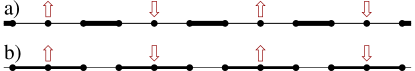
Figure 14: Valence Bond Solid states with period 3. Thick lines indicate stronger bonds. Remaining effective spin-1/2 degrees of freedom are also shown. Coexisting with the translational symmetry breaking, we have $1/x$ power law spin correlations with the antiferromagnetic (dynamic) pattern as shown. The two cases have slightly different microscopics, but are qualitatively similar on long length scales.

Continuing with the characterization, we note that $\vec{S}_{2k_{F1}}$ and all operators at $\pi/2$ have exponentially decaying correlations. On the other hand, $\vec{S}_{2k_{F2}}$ and ${\cal B}_{2k_{F2}}$ have $1/x$ power law correlations because of the remaining gapless $\theta_{2\sigma}$ mode. Since $2k_{F2}=\pi/3$, we have period-6 spin correlations on the original 1D chain.

The physical interpretation is simple. Consider first Fig. 14a) where every third bond is stronger. A caricature of this state is that spins in the strong bonds form singlets and are effectively frozen out. The remaining “free” spins are separated by three lattice spacings and are weakly antiferromagnetically coupled forming a new effective 1D chain. Thus we naturally have Bethe-chain-like staggered spin and bond energy correlations in this subsystem, which coexist with the static period-3 VBS order in the whole system. The situation in Fig. 14b) where every third bond is weaker is qualitatively similar. Here we can associate an effective spin-1/2 with each three-site cluster formed by strong bonds. These effective spins are again separated by three lattice spacings and form a new weakly coupled Bethe chain. Note that while the theory analysis has the Fermi wavevectors tuned to the commensuration, the resulting state is a stable phase that can occupy a finite region in the parameter space, as found by the DMRG in the ring model (see Sec. V.1).

We can construct trial wavefunctions using spinons as follows. In the mean field, we start with the band parameters $t_{1}$ and $t_{2}$ such that $k_{F1}=\pi/3$ and then add period-3 modulation of the hoppings. The $\pm k_{F1}$ Fermi points are connected by the modulation wavevector and are gapped out. The $\pm k_{F2}$ Fermi points remain gapless; just as in the Bethe chain case, the corresponding Bosonized field theory provides an adequate description of the long-wavelength physics, predicting $1/x$ decay of staggered spin and bond energy correlations.

The above wavefunction construction and theoretical analysis are implicitly in the regime where the residual spin correlations are antiferromagnetic. In a given physical system forming such a period-3 VBS, one can also imagine ferromagnetic residual interactions between the non-dimerized spins. Indeed, the DMRG finds some weak ferromagnetic tendencies in the ring model near the transition to this VBS state. This is not covered by our spin-singlet SBM theory but could possibly be covered starting with a partially polarized SBM state.

IV.5 Other possible commensurate points

Alerted by the period-3 VBS case, we look for and find one additional commensurate case with an allowed new interaction that can destabilize the Spin Bose-Metal. When $k_{F1}=3\pi/8$, we find a new quartic term

$$V_{4} \!=\! u_{4}\Big{[}f_{R1\uparrow}^{\dagger}f_{R1\downarrow}^{\dagger}\epsilon_{\alpha\beta}f_{L1\alpha}f_{R2\beta}+(R\leftrightarrow L)+{\rm H.c.}\Big{]}$$

$$\!\sim\! -i\eta_{1\uparrow}\eta_{2\uparrow}\sin(2\theta_{\rho-}+\theta_{\rho+}-\theta_{\sigma+})\sin(\varphi_{\rho-}+\varphi_{\sigma-})$$

$$-i\eta_{1\downarrow}\eta_{2\downarrow}\sin(2\theta_{\rho-}+\theta_{\rho+}+\theta_{\sigma+})\sin(\varphi_{\rho-}-\varphi_{\sigma-})~{}.$$

(For the schematic writing here, we have ignored the commutations of the fields when separating the $\varphi$’s and $\theta$’s.) The scaling dimension is $\Delta[V_{4}]=1/2+g+1/(4g)$. This is smaller than 2 for $g\in(0.191,1.309)$ and the interaction is relevant in this range. Since we have conjugate variables $\theta_{\rho-}$ and $\varphi_{\rho-}$ both present in the above potential, we can not easily determine the ultimate outcome of the runaway flow. It seems safe to assume that $\theta_{\sigma+}$ and $\varphi_{\sigma-}$ will be both pinned, which implies at least some period-2 translational symmetry breaking. One possibility, perhaps aided by the interactions Eq. (37), is that the $\varphi_{\rho-}$ is pinned; in this case, the situation is essentially the same as in Sec. IV.2.2 and we get some period-4 structure. Another possibility is that the $\theta_{\rho-}$ is pinned; in this case $\langle\epsilon_{4k_{F1}}\rangle\neq 0$, and since $4k_{F1}=-\pi/2$, we get period-4 bond pattern.

To conclude, we note that the commensurate cases in this section and in Sec. IV.4 can be understood phenomenologically by monitoring the wavevectors of the energy modes ${\cal B}_{Q}$. The dominant wavevectors are $\pm 2k_{Fa}$, $\pm\pi/2$, and $\pm 4k_{F2}=\mp 4k_{F1}$. When $4k_{F2}$ matches with $\pi/2$, we get the $k_{F1}=3\pi/8$ commensuration of this section (here also $2k_{F1}$ matches with $k_{F2}-k_{F1}$, while $2k_{F2}$ matches with $3k_{F1}+k_{F2}$). When $4k_{F2}$ matches with $2k_{F1}$, we get the $k_{F1}=\pi/3$ commensuration of the previous section. Tracking such singular wavevectors in the DMRG is then very helpful to alert us to possible commensuration instabilities, and both cases are realized in the ring model with additional antiferromagnetic $J_{3}=0.5J_{1}$ discussed in Sec. V.2, cf. Fig. 16.

V DMRG study of commensurate instabilities inside the SBM: VBS-3 and Chirality-4

V.1 Valence Bond Solid with period 3

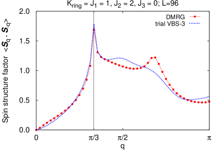
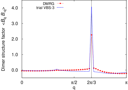
Figure 15: (Color online) Spin and dimer structure factors at a representative point in the VBS-3 phase, $K_{\rm ring}=J_{1}=1$, $J_{2}=2$, measured in the DMRG for system size $L=96$ (we do not show the chirality as it is not informative.) The most notable features are the dimer Bragg peak at $2\pi/3$ corresponding to the static VBS order and also the spin singularity at $\pi/3$ corresponding to the effective spin-1/2 chain formed by the non-dimerized spins, see Fig. 14. The trial VBS-3 wavefunction is constructed as described in the text.

As already mentioned in Sec. III, we find a range of parameters where the SBM phase is unstable towards a Valence Bond Solid with a period of 3 lattice spacings (VBS-3). In the model with $K_{\rm ring}=J_{1}=1$, this occurs for $1.5<J_{2}<2.5$, cf. Fig. 8. The characteristic correlations are shown in Fig. 15 at a point $J_{2}=2$. The dimer structure factor shows a Bragg peak at a wavevector $2\pi/3$ corresponding to the period-3 VBS order. The spin structure factor has a singularity at a wavevector $\pi/3$ corresponding to staggered correlations in the effective spin-1/2 chain formed by the non-dimerized spins, see Fig. 14. If we zoom in closer, the dimer structure factor also has a feature at $\pi/3$ that can be associated with this effective chain.

To construct a trial VBS-3 wavefunction, we start with the spinon hopping problem that would produce $k_{F1}=\pi/3$, so the first Fermi sea would be twice as large as the second. We then multiply every third first-neighbor hopping by $1+\delta$ and Gutzwiller-project; for the point in Fig. 15 we find optimal $\delta=1$. This gaps out the larger Fermi sea but leaves the smaller Fermi sea gapless. Our wavefunction is crude and shows a stronger dimer Bragg peak than the DMRG and somewhat different spin correlations at short scales, but otherwise captures the qualitative features as can be seen in Fig. 15.

The origin of the VBS-3 phase can be traced to the instability of the SBM at special commensuration, cf. Secs. IV.4-IV.5. Indeed, in Fig. 7 we can follow the evolution of the singular wavevectors in the SBM phase between the VBS-2 and VBS-3. As we decrease $J_{2}$ moving towards the VBS-3, the $4k_{F2}$ and $2k_{F1}$ singular wavevectors in the bond energy approach each other and coincide at $2\pi/3$. When this happens, there is a new umklapp term that can destabilize the SBM and produce the VBS-3 state as analyzed in Sec. IV.4. The instability requires $g<2/3$ for the SBM Luttinger parameter. In this case according to Table 1 the $4k_{F2}$ singularity in the dimer is stronger than the $2k_{F1,2}$, which is in agreement with what we see in the neighboring SBM in Fig. 7. The re-emergence of the $4k_{F2}$ and $2k_{F1}$ at the other end of the VBS-3 phase is obscured here by the weak ferromagnetic tendency (but is present in a model where this tendency is suppressed, see Fig. 16).

V.2 Enhancement of the spin-singlet SBM by antiferromagnetic third-neighbor coupling $J_{3}=0.5$ and a new phase with chirality order with period 4.

As discussed in Sec. III.3, in the original $J_{1}-J_{2}-K_{\rm ring}$ model, states in the SBM region near the left boundary of the VBS-3 tend to develop a small magnetic moment. We conjecture that this occurs in the second spinon Fermi sea and suggest that an antiferromagnetic $J_{3}$ will stabilize the SBM phase with spin-singlet ground state. One motivation comes from the picture of the neighboring VBS-3, where the non-dimerized spins are loosely associated with the second Fermi sea. These spins are three lattice spacings apart, so adding antiferromagnetic $J_{3}$ should lead to stronger antiferromagnetic tendencies among them and also in the physics associated with the second Fermi sea.

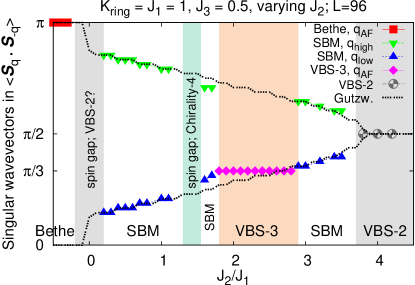
Figure 16: (Color online) Phase diagram of the $J_{1}-J_{2}-K_{\rm ring}$ model with additional antiferromagnetic third-neighbor coupling $J_{3}=0.5J_{1}$ introduced to stabilize spin-singlet states. The study is along the same cut $K_{\rm ring}=J_{1}$ as in Fig. 8, and the overall features are similar, with the following differences. The ground state is singlet throughout eliminating the difficult “partial FM” region to the left of the VBS-3 (and the VBS-3 phase is somewhat wider). There is a sizable spin-gapped region between the Bethe-chain and SBM phases (see text for more details). A new spin-gapped phase with period-4 chirality order appears inside the SBM to the left of the VBS-3.

We have performed a detailed study adding a modest $J_{3}=0.5$ to the original model Eq. (1) along the same cut $K_{\rm ring}=J_{1}=1$. Our motivating expectations are indeed borne out. Figure 16 shows the phase diagram together with the evolution of the singular wavevectors as a function of $J_{2}/J_{1}$. While the overall features are similar to the phase diagram in the $J_{3}=0$ case, Fig. 8, a few points are worth mentioning.

First, the partial spin polarization is absent in the whole SBM phase between the Bethe-chain and VBS-3 phases. The DMRG converges confidently to spin-singlet ground state for $L=96$. All properties are similar to those in Figs. 4 and 6, providing further support for the singlet SBM phase in the original $J_{3}=0$ model. The VBS-3 phase and the SBM phase between the VBS-3 and VBS-2 are qualitatively very similar in the two cases $J_{3}=0$ and $J_{3}=0.5$ and are not discussed further here.

An interesting feature in the model with $J_{3}=0.5$ is the presence of a sizable phase with spin gap intervening between the Bethe-chain and SBM phases. Our best guess is that this phase has period-2 VBS order, although we do not see a clear signature in the dimer correlations. Our DMRG states in this region show very weak (if any) dimerization of the first-neighbor bonds, which may explain the lack of clear order in these dimer correlations. On the other hand, we see a sizable period-2 dimerization of the third-neighbor bonds $\langle\vec{S}(x)\cdot\vec{S}(x+3)\rangle$, but have not measured the corresponding bond-bond correlations to confirm long-range order. We have not explored possible theoretical routes to understand the origin of this phase yet and leave our discussion of this region as is.

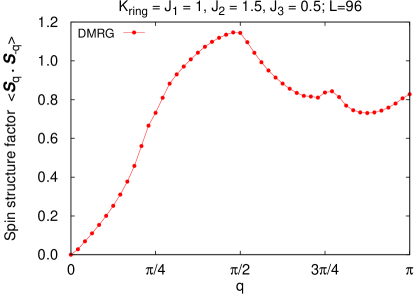
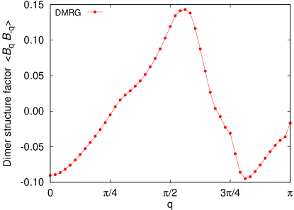
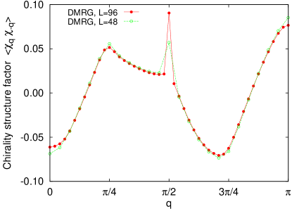
Figure 17: (Color online) Spin, dimer, and chirality structure factors at a point in the tentative Chirality-4 phase, $K_{\rm ring}=J_{1}=1$, $J_{2}=1.5,J_{3}=0.5$, measured in the DMRG for system size $L=96$. Note the absence of sharp features in the spin correlations, which suggests a spin gap, while the dimer correlations have only a feature at $\pi$ corresponding to period-2 modulation. On the other hand, the chirality structure factor shows a Bragg peak at $\pi/2$ that grows with increasing system size. The pattern of chirality correlations in real space is consistent with the order shown in Fig. 13.

We now turn to one more new phase found in the $J_{3}=0.5$ model. In a narrow region inside the SBM phase not far from the left end of the VBS-3, we again find a spin-gapped phase. We identify this as having period-4 order in the chirality (Chirality-4 phase). Figure 17 presents a point $J_{2}=1.5,J_{3}=0.5$. Looking at the singular wavevectors in Fig. 16, we see that this point is roughly where $q_{\rm low}=2k_{F2}$ passes $\pi/4$. Analysis in Sec. IV.5 suggests an instability gapping out all modes and leading to some period-4 structure. Indeed, the DMRG spin and dimer structure factors show only some remnants of features near $2k_{F1},2k_{F2}$, while the chirality shows a sharp peak at $\pi/2$. Looking at real space correlations, our $L=96$ DMRG state breaks translational symmetry. The pattern of chirality correlations is consistent with the period-4 order shown in Fig. 13. The pattern of dimer correlations is also consistent with this picture and shows modulation with period 2, which can be seen as a feature at $\pi$ in the dimer structure factor in Fig. 17.

To summarize, with the help of modest $J_{3}=0.5$ we have stabilized the spin-singlet SBM states between the Bethe-chain and VBS-3 phases. By suppressing potential weak ferromagnetism, we have uncovered the Chirality-4 phase, which can be understood as arising from the instability of the SBM at the special commensuration discussed in Sec. IV.5.

VI An attempt to bring out partially magnetized Spin Bose-Metal by ferromagnetic third neighbor coupling $J_{3}=-0.5$

In the original model Eq. (1), we do not have a clear understanding of the “partial FM” states to the left of the VBS-3 phase in Fig. 2. As discussed in Sec. III.3, we suspect that there is a tendency to weak ferromagnetism in the second Fermi sea. However, the magnetizations that we measure are not large: e.g., they are significantly smaller than if we were to fully polarize the second Fermi sea, and it is difficult to analyze such states. Here we seek better control over the spin polarization by adding modest ferromagnetic $J_{3}=-0.5$ in hopes of stabilizing states with a full spontaneous polarization of the second Fermi sea, which is easier to analyze.

We do not have as detailed phase diagram as for the $J_{3}=0$ and $J_{3}=0.5$ cases. We expect it to look crudely similar to Figs. 8 and 16, with a narrower (if any) VBS-3 region, and with a wider partially polarized SBM region. We indeed find stronger ferromagnetic tendencies in the range $0\leq J_{2}\leq 2$. However, we cannot claim achieving robust full polarization of the second Fermi sea and understanding all behavior. The largest magnetization and properties closest to our expectations are found in the middle region near $J_{2}\simeq 1$. With this cautionary note warranting more work, we now present results for $J_{2}\simeq 1$ to illustrate our thinking about such states.

The DMRG study proceeds as follows. We start as before working in the $S^{z}_{\rm tot}=0$ sector. We measure the spin structure factor and calculate the total spin $S_{\rm tot}$ from Eq. (32), which can give a first indication of a non-zero magnetization. However, for the larger system sizes, the DMRG finds it difficult to converge to integer-valued $S_{\rm tot}$ due to a mixing of states with different total spins, and this leads to significant uncertainty. To check the value of the ground state spin, we run the DMRG in sectors with different $S^{z}_{\rm tot}$, expecting the ground state energy to be the same for $S^{z}_{\rm tot}=0,\dots,S_{\rm tot}$ and then to jump to a higher value for $S^{z}_{\rm tot}>S_{\rm tot}$.

As an example, at a point $J_{2}=1$ for system size $L=48$ we find that the DMRG energy is the same in the sectors $S^{z}_{\rm tot}=0,\dots,5$ and then jumps, so the ground state spin is determined as $S_{\rm tot}=5$. The DMRG convergence is good and the SU(2)-invariant structure factor $\langle\vec{S}_{q}\cdot\vec{S}_{-q}\rangle$ is the same measured in the different sectors $S^{z}_{\rm tot}\leq 5$, indicating that these states indeed belong to the same multiplet.

The situation is less clear for $L=96$ because of reduced convergence. At the point $J_{2}=1$ the extensive energies obtained by the DMRG in the sectors $S^{z}_{\rm tot}=0,\dots,10$ are non-systematic and are within $0.1J_{1}$ of each other, with the lowest energy found in the $S^{z}_{\rm tot}=10$ sector. Also, the SU(2)-invariant structure factors differ slightly and the estimates of $S_{\rm tot}$ vary around $S_{\rm tot}\sim 8-10$. The convergence is best in the highest $S^{z}_{\rm tot}=10$ sector, where the total spin is found to be accurately $S_{\rm tot}=10$; the improved convergence is indeed expected since there are fewer available low energy excited states to mix with (e.g., spin-wave excitations of the ferromagnet are not present in the highest $S^{z}$ sector). Interestingly, we find a fully converged state in the $S^{z}_{\rm tot}=11$ sector with $S_{\rm tot}=11$ whose energy is only slightly higher, which probably adds to the above convergence difficulties. More importantly, the energy jumps to a significantly higher value in the sector $S^{z}_{\rm tot}=12$. Our best conclusion is that the total spin of the ground state is $S_{\rm tot}=10$.

Turning to the VMC study, we consider a family of variational Gutzwiller states where we allow different spin up and spin down populations of the two Fermi seas centered around $k=0$ and $\pi$ (we do not attempt any further improvements on top of such bare wavefunctions). In the model parameter region discussed here, we find that the optimal such states have a fully polarized second Fermi sea and an unpolarized first Fermi sea. For the $L=48$ example quoted above, the optimal VMC polarization indeed matches the DMRG $S_{\rm tot}=5$, while for the $L=96$ case the optimal VMC state has $S_{\rm tot}=11$ and a state with $S_{\rm tot}=10$ is very close in energy. Appendix B.3 provides more details on the properties of such Gutzwiller states, while here we simply compare the VMC and DMRG measurements.

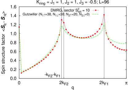
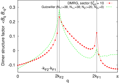
Figure 18: (Color online) Spin and dimer structure factors at a tentative point with partial ferromagnetism, $K_{\rm ring}=J_{1}=1$, $J_{2}=1$, $J_{3}=-0.5$, measured in the DMRG for system size $L=96$. The calculations are done in the sector $S^{z}_{\rm tot}=10$ where the DMRG is well-converged and gives $S_{\rm tot}=10$, which we think is the true ground state spin. The VMC state has the second Fermi sea fully polarized with $N_{2\uparrow}=20,N_{2\downarrow}=0$, while the first Fermi sea is unpolarized with $N_{1\uparrow}=N_{1\downarrow}=38$. Vertical lines label important wavevectors $2k_{F1}$, $2k_{F2}$, and $-k_{F2}-k_{F1}$.

The DMRG structure factors for the $J_{2}=1,J_{3}=-0.5$, $L=96$ system are shown in Fig. 18, together with the VMC results for the Gutzwiller wavefunction with $S_{\rm tot}=10$. A notable difference from the singlet SBM states of Sec. III is that the characteristic peaks are no longer located symmetrically about $\pi/2$. For example, in the trial state we have prominent wavevectors $2k_{F2}$ and $2k_{F1}$ that satisfy $2k_{F2}+2\times 2k_{F1}=2\pi$; also, we have a wavevector $-k_{F2}-k_{F1}$, which is now different from $\pi/2$. It is not easy to discern all wavevectors in Fig. 18 because the $2k_{F2}$ happens to be close with the $-k_{F2}-k_{F1}$. Nevertheless, the overall match between the DMRG and VMC suggests that the trial wavefunction captures reasonably the nature of the ground state.

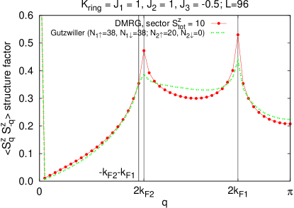
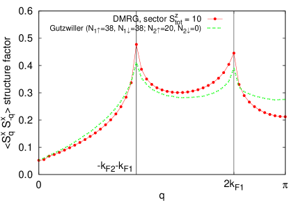
Figure 19: (Color online) Separate $\langle S^{z}_{q}S^{z}_{-q}\rangle$ and $\langle S^{x}_{q}S^{x}_{-q}\rangle$ structure factors for the same system as in Fig. 18.

Working in the sector $S^{z}_{\rm tot}=S_{\rm tot}$ also allows more detailed comparison between the DMRG and VMC. In this case, there is a sharp distinction between the $\langle S^{z}_{q}S^{z}_{-q}\rangle$ and $\langle S^{x}_{q}S^{x}_{-q}\rangle$ structure factors. The former has singular wavevectors $2k_{F1}$, $2k_{F2}$, and $-k_{F2}-k_{F1}$, while the latter is lacking the wavevector $2k_{F2}$ since there is no spin-flip process across the second Fermi sea. Our measurements are shown in Fig. 19. The wavevectors $2k_{F2}$ and $-k_{F2}-k_{F1}$ are too close to make a more clear-cut distinction; nevertheless, the VMC reproduces all details quite well.

In analogy with the SBM theory, we expect the $2k_{F1}$ and $2k_{F2}$ singularities to become stronger compared with the bare Gutzwiller and the $-k_{F2}-k_{F1}$ to become weaker; this is roughly consistent with what we see in the DMRG structure factors. As discussed in Appendix B.3, however, we do not have a complete description of such a partially polarized SBM phase that must incorporate ferromagnetic spin waves as well as the low energy SBM modes. This is left for future work. We also mention that the closeness of the $2k_{F2}$ and $-k_{F2}-k_{F1}$ warns us that the system is near a commensuration point with $k_{F1}=2\pi/5$ where it can be further unstable, which requires more study.

To summarize, by adding modest ferromagnetic $J_{3}=-0.5$ we have realized the SBM state with fully polarized second Fermi sea, confirming our intuition about the origin of the weak ferromagnetic tendencies in the original model discussed in Sec. III.3. A more thorough exploration of the phase diagram in the model with $J_{3}=-0.5$ as well as in the original model in the partial FM region is clearly warranted to develop better understanding of such partially ferromagnetic states.

VII Conclusions and future directions

We have summarized the main results and presented much discussion particularly in Sec. I. Perhaps one point we would like to reiterate is the remarkable coincidence between the sign structure present in the DMRG wavefunctions for the spin model SBM phase and the sign structure in the spin sector of free fermions on the ladder (e.g., metallic electrons). This sign structure is encoded in the singular wavevectors (“Bose surfaces”), and indeed the Gutzwiller-projected wavefunction with just one variational parameter is sufficient to reproduce the locations of all the singularities throughout the observed SBM phase.

We conclude by mentioning some standing questions and future directions. First, in the ring model, we have focused on the Spin Bose-Metal and dealt with other phases only as needed to sketch the rich phase diagram. For example, we have not studied carefully the VBS-2 region, which might harbor additional phases. We have not studied adequately (numerically or analytically) the spin-gap region between the Bethe-chain and SBM phases in the $J_{3}=0.5$ model, Fig. 16. One question to ask here is whether there is a generic instability when we start populating the second Fermi sea, or whether we can go directly from the Bethe-chain phase to the SBM. More generally, we have not studied various phase transitions in the system.

Next, while we understand the long-wavelength SBM theory with its single Luttinger parameter $g$, we have found that the Gutzwiller wavefunctions represent only the special case $g=1$ and cannot capture the general situation $g<1$. It would clearly be desirable to construct spin-singlet wavefunctions appropriate for the general case. Even thinking about the Gutzwiller wavefunctions, it could be interesting to understand the observed $g=1$ analytically and ask if they may be exact ground states of some Hamiltonians (in the spirit of the Haldane-Shastry modelHaldane (1988); Shastry (1988)).

On a separate front, we have encountered an interesting possibility of the Spin Bose-Metal with partial ferromagnetism occurring in one of the subbands, but more work is needed to fully understand the numerical observations and develop analytical theory. Even without a spontaneous moment in the ground state, our observations suggest that in the regime between the Bethe-chain and VBS-3 phases the second band is narrow in energy. Some ferromagnetic instability or possibility of spin-incoherent regime in one of the bands can lead to anomalous transport properties in such a quantum wire, a topic of much current interest. Meyer and Matveev (2009); Matveev (2004a, b); Fiete (2007)

Looking into future, it will be interesting to consider electron Hubbard-like models on the two-leg triangular strip and look for possible SBM phase. The Hubbard model has been studied in a number of works, Daul and Noack (2000); Louis et al. (2001); Capello et al. (2005); Japaridze et al. (2007) but the focus has been mainly on the conventional insulating phases such as the Bethe-chain and VBS-2 states. This is appropriate in the strong Mott insulator limit, $t_{1},t_{2}\ll U$, where the effective spin model is the $J_{1}-J_{2}$ model with $J_{1}=2t_{1}^{2}/U$, $J_{2}=2t_{2}^{2}/U$. However, at intermediate coupling just on the insulator side, one needs to include multiple-spin exchanges, and the leading new term is the ring exchange with $K_{\rm ring}=20t_{1}^{2}t_{2}^{2}/U^{3}$. As we have learned, this ring term stabilizes the SBM phase, so revisiting the Hubbard model with the insights gained here is promising. In Sec. II.2, we approached the SBM by starting with a metallic two-band electron system (“C2S2”) and gapping out only the overall charge mode “$\rho+$”. Then it is natural to look for the SBM near an extended such C2S2 metallic phase, and we may need to consider electron models with further-neighbor repulsion to open wider windows of such phases.

Last but not least, we would like to advance the program of ladder studies closer to 2D. It is prudent to focus on the spin model with ring exchanges. On the exact numerics front, 4 to 6 legs is probably at the limit of the DMRG capabilities. The VMC approach should still be able to capture the critical surfaces if they are present, since they are dictated by short-distance physics; on the other hand, the bare Gutzwiller will likely fail even more in reproducing correct long-distance behavior. We do not know how far the present Bosonization approach can sensibly hold going to more legs. These are challenging but worthwhile endeavors given the experimental importance of understanding weak Mott insulators.

Appendix A Observables in the SBM phase

We have defined spin $\vec{S}(x)$, bond energy ${\cal B}(x)$, and chirality $\chi(x)$ observables in Sec. II.3 [cf. Eqs. (22-23)]. Here we find detailed Bosonized forms by a systematic construction of observables in the SBM (and will find more observables on the way).

In the gauge theory treatment Sec. II.1, we consider gauge-invariant objects constructed from the spinon fields; in the interacting electron picture of Sec. II.2, these are operators that do not change the total charge.

We begin with fermion bilinears and first consider the ones composed of a particle and a hole moving in opposite directions. Such bilinears are expected to be enhanced by gauge fluctuations since parallel gauge currents experience Amperean attraction. We organize these bilinears as follows:

$$\vec{S}_{2k_{Fa}} \equiv \frac{1}{2}f^{\dagger}_{La\alpha}\vec{\sigma}_{\alpha\beta}f_{Ra\beta}~{},$$ (66)

$$\epsilon_{2k_{Fa}} \equiv \frac{1}{2}f^{\dagger}_{La\alpha}f_{Ra\alpha}~{},$$ (67)

$$\vec{S}_{\pi/2} \equiv \frac{1}{2}f^{\dagger}_{R1\alpha}\vec{\sigma}_{\alpha\beta}f_{L2\beta}+\frac{1}{2}f^{\dagger}_{R2\alpha}\vec{\sigma}_{\alpha\beta}f_{L1\beta}~{},$$ (68)

$$\epsilon_{\pi/2} \equiv \frac{1}{2}f^{\dagger}_{R1\alpha}f_{L2\alpha}+\frac{1}{2}f^{\dagger}_{R2\alpha}f_{L1\alpha}~{},$$ (69)

$$\vec{\delta}_{\pi/2} \equiv \frac{1}{2}f^{\dagger}_{R1\alpha}\vec{\sigma}_{\alpha\beta}f_{L2\beta}-\frac{1}{2}f^{\dagger}_{R2\alpha}\vec{\sigma}_{\alpha\beta}f_{L1\beta}~{},$$ (70)

$$\chi_{\pi/2} \equiv \frac{1}{2}f^{\dagger}_{R1\alpha}f_{L2\alpha}-\frac{1}{2}f^{\dagger}_{R2\alpha}f_{L1\alpha}~{},$$ (71)

with $\vec{S}_{-Q}=\vec{S}_{Q}^{\dagger}$, etc. The microscopic spin operator expanded in terms of the continuum fermion fields readily gives the listed $\vec{S}_{Q}$.

The bond energy can be approximated as the spinon hopping energy,

$${\cal B}(x)\sim-t[f_{\alpha}^{\dagger}(x)f_{\alpha}(x+1)+{\rm H.c.}]$$ (72)

(recall that we work in the gauge with zero spatial vector potential). Expansion in terms of the continuum fields gives, up to a real factor,

$${\cal B}_{Q}\sim e^{iQ/2}\epsilon_{Q}~{}.$$ (73)

Such connection between ${\cal B}_{Q}$ and $\epsilon_{Q}$ is understood below for all $Q\neq\pi$. The objects $\epsilon_{Q}$ are convenient because of their simpler transformation properties under lattice inversion, $\epsilon_{Q}\leftrightarrow\epsilon_{-Q}$.

The physical meaning of the operators $\vec{\delta}_{\pi/2}$ and $\chi_{\pi/2}$ can be established on symmetry grounds. Thus, $\chi$ is the spin chirality defined in Eq. (23). The expression in terms of bilinears can be also found directly by considering the circulation of the gauge charge current around the $[x-1,x,x+1]$ loop,

$$\chi(x) \sim \circlearrowleft\sum it_{rr^{\prime}}[f_{\alpha}^{\dagger}(r)f_{\alpha}(r^{\prime})-{\rm H.c.}]~{}.$$ (74)

This is familiar in slave particle treatments:Lee et al. (2006) the circulation produces internal gauge flux whose physical meaning is the spin chirality. On the other hand, $\vec{\delta}$ is related to the following microscopic operator;

$$\vec{D}(x)=\vec{S}(x)\times\vec{S}(x+1)~{},\quad\vec{D}_{\pi/2}=e^{i\pi/4}\vec{\delta}_{\pi/2}~{}.$$ (75)

At $Q=\pi/2$, this enters on par with $\vec{S}$, ${\cal B}$, and $\chi$.

The bosonized expressions at the $2k_{Fa}$ are:

$$S^{x}_{2k_{Fa}} = -i\eta_{a\uparrow}\eta_{a\downarrow}e^{i\theta_{\rho+}}e^{\pm i\theta_{\rho-}}\sin(\sqrt{2}\varphi_{a\sigma})~{},$$ (76)

$$S^{y}_{2k_{Fa}} = -i\eta_{a\uparrow}\eta_{a\downarrow}e^{i\theta_{\rho+}}e^{\pm i\theta_{\rho-}}\cos(\sqrt{2}\varphi_{a\sigma})~{},$$ (77)

$$S^{z}_{2k_{Fa}} = -e^{i\theta_{\rho+}}e^{\pm i\theta_{\rho-}}\sin(\sqrt{2}\theta_{a\sigma})~{},$$ (78)

$$\epsilon_{2k_{Fa}} = ie^{i\theta_{\rho+}}e^{\pm i\theta_{\rho-}}\cos(\sqrt{2}\theta_{a\sigma})~{},$$ (79)

where the upper or lower sign in the exponent corresponds to $a=1$ or $2$. The pinned value $\theta_{\rho+}$, which is determined by minimizing Eq. (17), is left general at this stage. It is not so important for the qualitative behavior at the $2k_{Fa}$ and $\pi/2$, but is crucial at a wavevector $\pi$ later.

For each $a$, the $(\vec{S},{\cal B})_{2k_{Fa}}$ structure is similar to that in a single Bethe chain except for the $\theta_{\rho}$ exponentials. As in the Bethe chain, we expect the spin and VBS correlations to be closely related – in particular, they decay with the same power law. The corresponding scaling dimension in the fixed-point theory Eq. (18) is

$$\Delta[\vec{S}_{2k_{Fa}}]=\Delta[{\cal B}_{2k_{Fa}}]=\frac{1}{2}+\frac{g}{4}~{}.$$ (80)

The bosonized expressions at the $\pi/2$ are:

$$S^{x}_{\pi/2} = e^{-i\theta_{\rho+}}\Big{[}-i\eta_{1\uparrow}\eta_{2\downarrow}e^{-i\theta_{\sigma-}}\sin(\varphi_{\rho-}+\varphi_{\sigma+})$$ (82)

$$~{}~{}~{}~{}~{}~{}~{}~{}~{}-i\eta_{1\downarrow}\eta_{2\uparrow}e^{i\theta_{\sigma-}}\sin(\varphi_{\rho-}-\varphi_{\sigma+})\Big{]}~{},$$

$$S^{y}_{\pi/2} = e^{-i\theta_{\rho+}}\Big{[}-i\eta_{1\uparrow}\eta_{2\downarrow}e^{-i\theta_{\sigma-}}\cos(\varphi_{\rho-}+\varphi_{\sigma+})$$ (84)

$$~{}~{}~{}~{}~{}~{}~{}~{}~{}+i\eta_{1\downarrow}\eta_{2\uparrow}e^{i\theta_{\sigma-}}\cos(\varphi_{\rho-}-\varphi_{\sigma+})\Big{]}~{},$$

$$S^{z}_{\pi/2} = e^{-i\theta_{\rho+}}\Big{[}-i\eta_{1\uparrow}\eta_{2\uparrow}e^{-i\theta_{\sigma+}}\sin(\varphi_{\rho-}+\varphi_{\sigma-})$$ (86)

$$~{}~{}~{}~{}~{}~{}~{}~{}~{}+i\eta_{1\downarrow}\eta_{2\downarrow}e^{i\theta_{\sigma+}}\sin(\varphi_{\rho-}-\varphi_{\sigma-})\Big{]}~{},$$

$$\epsilon_{\pi/2} = e^{-i\theta_{\rho+}}\Big{[}-i\eta_{1\uparrow}\eta_{2\uparrow}e^{-i\theta_{\sigma+}}\sin(\varphi_{\rho-}+\varphi_{\sigma-})$$ (88)

$$~{}~{}~{}~{}~{}~{}~{}~{}~{}-i\eta_{1\downarrow}\eta_{2\downarrow}e^{i\theta_{\sigma+}}\sin(\varphi_{\rho-}-\varphi_{\sigma-})\Big{]}~{},$$

$$\chi_{\pi/2} = e^{-i\theta_{\rho+}}\Big{[}-\eta_{1\uparrow}\eta_{2\uparrow}e^{-i\theta_{\sigma+}}\cos(\varphi_{\rho-}+\varphi_{\sigma-})~{}~{}~{}~{}~{}~{}~{}~{}$$ (90)

$$~{}~{}~{}~{}~{}~{}~{}~{}~{}-\eta_{1\downarrow}\eta_{2\downarrow}e^{i\theta_{\sigma+}}\cos(\varphi_{\rho-}-\varphi_{\sigma-})\Big{]}~{}.~{}~{}~{}~{}~{}~{}~{}~{}$$

Expressions for $\vec{\delta}_{\pi/2}$ can be obtained from those for $\vec{S}_{\pi/2}$ essentially by interchanging sines and cosines. As before, ${\cal B}_{\pi/2}$ is given by Eq. (73). The above details are needed particularly when we discuss phases arising as instabilities of the SBM, Secs. IV.2-IV.5, while in the SBM we immediately see that all scaling dimensions are equal:

$$\Delta[\vec{S}_{\pi/2}]=\Delta[{\cal B}_{\pi/2}]=\Delta[\vec{D}_{\pi/2}]=\Delta[\chi_{\pi/2}]=\frac{1}{2}+\frac{1}{4g}~{}.$$ (91)

This completes the “enhanced” bilinears. We also mention, without giving detailed expressions, “non-enhanced” bilinears at wavevectors $Q=\pm(k_{F2}-k_{F1})$. Their scaling dimension is

$$\Delta[\vec{S}_{Q}]=\Delta[{\cal B}_{Q}]=\Delta[\vec{D}_{Q}]=\Delta[\chi_{Q}]=\frac{1}{2}+\frac{1}{4g}+\frac{g}{4}~{},$$ (92)

which is always larger than the spinon mean field value of $1$.

Finally, we have bilinears carrying zero momentum – essentially $J_{Paa},\vec{J}_{Paa}$ from Eq. (34). These give conserved densities and currents and have scaling dimension $1$. We specifically mention examples leading to Eqs. (25-27):

$$S^{z}_{Q=0}\sim J^{z}_{R11}+J^{z}_{L11}+J^{z}_{R22}+J^{z}_{L22}=\frac{1}{\pi}\partial_{x}\theta_{\sigma+}~{},$$ (93)

$$\epsilon_{Q=0}\sim J_{R11}+J_{L11}-J_{R22}-J_{L22}=\frac{2}{\pi}\partial_{x}\theta_{\rho-}~{},$$ (94)

$$\chi_{Q=0}\sim J_{R11}-J_{L11}-J_{R22}+J_{L22}=\frac{2}{\pi}\partial_{x}\varphi_{\rho-}~{}.$$ (95)

(One way we can make the identifications in the last two lines is by using physical symmetry arguments.)

So far, we have only considered fermion bilinears. Since the theory is strongly coupled, we should also study contributions with more fermion fields. We now include four-fermion terms focusing on the spin, bond energy, and chirality operators that are measured in the DMRG. First, there appears a new wavevector $4k_{F1}=-4k_{F2}$ in the bond energy, via,

$$\epsilon_{4k_{F1}}: f_{L1\uparrow}^{\dagger}f_{L1\downarrow}^{\dagger}f_{R1\uparrow}f_{R1\downarrow}\sim e^{i2\theta_{\rho+}}e^{i2\theta_{\rho-}}~{},$$ (97)

$$f_{R2\uparrow}^{\dagger}f_{R2\downarrow}^{\dagger}f_{L2\uparrow}f_{L2\downarrow}\sim e^{-i2\theta_{\rho+}}e^{i2\theta_{\rho-}}~{}.$$

The two contributions come with independent numerical factors and can be also generated as $(\epsilon_{2k_{F1}})^{2}$ and $(\epsilon_{-2k_{F2}})^{2}$. Once the $\theta_{\rho+}$ is pinned, there is only one qualitatively distinct contribution and the scaling dimension is

$$\Delta[{\cal B}_{4k_{F1}}]=g~{}.$$ (98)

Note that for sufficiently small $g<2/3$, the power law decay is slower than that of the bilinears ${\cal B}_{2k_{Fa}}$. There is no comparable $4k_{F1}$ contribution to the spin operator.

Four-fermion terms bring out another important wavevector, $Q=\pi$. We list independent dominant such contributions to $\vec{S}_{\pi}$, ${\cal B}_{\pi}$, and $\chi_{\pi}$:

$$S^{z}_{\pi}: \sin(2\theta_{\sigma+})\sin(2\theta_{\rho+})~{},\;\;\sin(2\theta_{\sigma-})\sin(2\theta_{\rho+})~{};~{}~{}~{}~{}~{}$$ (99)

$${\cal B}_{\pi}: [\cos(2\theta_{\sigma+})+\cos(2\theta_{\sigma-})]\sin(2\theta_{\rho+})~{},$$ (102)

$$[\cos(2\theta_{\sigma+})+\hat{\Gamma}\cos(2\varphi_{\sigma-})]\sin(2\theta_{\rho+})~{},$$

$$\hat{\Gamma}\cos(2\varphi_{\rho-})\sin(2\theta_{\rho+})~{};$$

$$\chi_{\pi}: \hat{\Gamma}\sin(2\varphi_{\rho-})\sin(2\theta_{\rho+})~{}.$$ (103)

These can be generated by combining the previously exhibited bilinears as follows. $S^{z}_{\pi}$: $S^{z}_{2k_{F1}}\epsilon_{2k_{F2}}\pm S^{z}_{2k_{F2}}\epsilon_{2k_{F1}}+{\rm H.c.}$; ${\cal B}_{\pi}$: $i\epsilon_{2k_{F1}}\epsilon_{2k_{F2}}+{\rm H.c.}$, $i(\epsilon_{\pi/2}^{2}-\chi_{\pi/2}^{2})+{\rm H.c.}$, $i(\epsilon_{\pi/2}^{2}+\chi_{\pi/2}^{2})+{\rm H.c.}$; $\chi_{\pi}$: $\chi_{\pi/2}\epsilon_{\pi/2}+{\rm H.c.}$ The scaling dimensions are

$$\Delta[\vec{S}_{\pi}] = \Delta[{\cal B}_{\pi}]=1~{},$$ (104)

$$\Delta[\chi_{\pi}] = 1/g~{}.$$ (105)

The above observables are present if $\sin(2\theta_{\rho+})\neq 0$, e.g., if the $\theta_{\rho+}$ is pinned as in Eq. (14), which we argued is natural when the spin model is describing a Mott insulator phase of a repulsive electron model. On the other hand, the above contributions would vanish if the pinning potential Eq. (17) had $v_{8}<0$. Some other physical observables containing $\cos(2\theta_{\rho+})$ and having different symmetry properties would be present instead. We do not write these out since both the DMRG and the trial wavefunctions have signatures in the spin, VBS, and chirality at the wavevector $\pi$, suggesting that the pinning Eq. (14) is realized. We have identified several more new observables at $\pi$ containing $\sin(2\theta_{\rho+})$; we do not spell these out here since our primary focus is to understand features in the numerics measuring the familiar $\vec{S}$, ${\cal B}$, and $\chi$.

We finally mention that four-fermion terms produce still more wavevectors, $\pm(3k_{F1}+k_{F2})=\mp(3k_{F2}+k_{F1})$; for example, $3k_{F1}+k_{F2}$ can be obtained by combining $2k_{F1}$ and $-\pi/2$. The scaling dimensions are the same as at $\pm(k_{F2}-k_{F1})$, Eq. (92).

For completeness, we have also checked six-fermion and eight-fermion terms. The only new wavevectors where the scaling dimension can be smaller than $2$ are $6k_{Fa}=2k_{Fa}+4k_{Fa}$ (scaling dimension $1/2+9g/4$), and $8k_{Fa}=4k_{Fa}+4k_{Fa}$ (scaling dimension $4g$). However, one needs small $g$ for these to become visible and in any case they always have faster power law decay than at $2k_{Fa}$ and $4k_{Fa}$. Finally, entries listed as “subd.” in Table 1 can be constructed, e.g., as $\chi_{Q}\sim\chi_{0}\epsilon_{Q}$, which has scaling dimensions $1+\Delta[\epsilon_{Q}]$.

Table 1 summarizes our results for the correlations in the Spin Bose-Metal phase. In words, we expect dominant spin and VBS correlations at the wavevectors $\pm 2k_{F1}$, $\pm 2k_{F2}$ decaying as $1/x^{1+g/2}$ and at the wavevectors $\pm\pi/2$ decaying as $1/x^{1+1/(2g)}$. The former decay is more slow since stability of the phase requires $g<1$. Note that the wavevectors $2k_{F1}$ and $2k_{F2}$ are located symmetrically around $\pi/2$. We also expect a $1/x^{2}$ power law at the wavevectors $0$ and $\pi$. Next, at the wavevectors $\pm(k_{F2}-k_{F1})$ and $\pm(3k_{F1}+k_{F2})$, which are also located symmetrically around $\pm\pi/2$, we expect a still faster power law $1/x^{1+1/(2g)+g/2}$. Furthermore, the bond energy shows a power law $1/x^{2g}$ at $\pm 4k_{F1}$. The spin chirality has similar signatures to the above at $\pm\pi/2$, $0$, $\pm(k_{F2}-k_{F1})$, and $\pm(3k_{F1}+k_{F2})$, but decays as $1/x^{2/g}$ at $\pi$. These are the simplest observables that can be used to identify the SBM phase in a given system. Figure 21 shows measurements in the Gutzwiller wavefunction projecting two Fermi seas and nicely illustrates all singular wavevectors, while it appears that such wavefunctions realize a special case with $g=1$. We also remark that in the general SBM the presence of the marginally irrelevant interactions Eq. (43) will lead to logarithmic corrections in correlations. Singh et al. (1989); Affleck et al. (1989)

We conclude by describing our treatment of the Klein factors (see, e.g., Ref. Fjaerestad and Marston, 2002 for more details). We need this when determining “order parameters” of various phases obtained as instabilities of the SBM, Secs. IV.2-IV.5. The operator $\hat{\Gamma}$ from Eq. (40) has eigenvalues $\pm 1$. For concreteness, we work with the eigenstate corresponding to $+1$: $\hat{\Gamma}|+\rangle=|+\rangle$. We then find the following relation

$$\langle+|\eta_{1\uparrow}\eta_{2\uparrow}|+\rangle=\langle+|\eta_{1\downarrow}\eta_{2\downarrow}|+\rangle=\textrm{pure imaginary}~{}.$$ (106)

This is useful when discussing observables at the $\pm\pi/2$ wavevectors; for example,

$$\epsilon_{\pi/2} \!\!=\!\! -e^{-i\theta_{\rho+}}\langle+|\eta_{1\uparrow}\eta_{2\uparrow}|+\rangle\Big{[}\cos(\varphi_{\rho-})\sin(\theta_{\sigma+})\sin(\varphi_{\sigma-})$$ (107)

$$~{}~{}~{}~{}~{}~{}~{}~{}~{}~{}~{}~{}~{}~{}~{}~{}~{}+i\sin(\varphi_{\rho-})\cos(\theta_{\sigma+})\cos(\varphi_{\sigma-})\Big{]}~{},$$

$$\chi_{\pi/2} \!\!=\!\! -e^{-i\theta_{\rho+}}\langle+|\eta_{1\uparrow}\eta_{2\uparrow}|+\rangle\Big{[}\cos(\varphi_{\rho-})\cos(\theta_{\sigma+})\cos(\varphi_{\sigma-})$$ (108)

$$~{}~{}~{}~{}~{}~{}~{}~{}~{}~{}~{}~{}~{}~{}~{}~{}~{}+i\sin(\varphi_{\rho-})\sin(\theta_{\sigma+})\sin(\varphi_{\sigma-})\Big{]}~{}.$$

Appendix B Details of the wavefunctions

B.1 Gutzwiller projection of two Fermi seas

It is convenient to view the spin wavefunction as that of hard-core bosons, where up/down spin corresponds to present/absent boson. In the general spinon construction, we occupy $\{k^{\uparrow}_{j},j=1,\dots,N_{\uparrow}\}$ orbitals with spin up and $\{k^{\downarrow}_{j},j=1,\dots,N_{\downarrow}\}$ orbitals with spin down; $N_{\uparrow}+N_{\downarrow}=L$ is the size of the system. After the Gutzwiller projection, the boson wavefunction is

$$\Psi_{\rm bos}(\{R_{i},i=1,\dots,N_{\uparrow}\})=\det[e^{ik^{\uparrow}_{j}R_{i}}]\det[e^{ip_{j}R_{i}}]~{},$$ (109)

where the set $\{p_{j},j=1,\dots,N_{\uparrow}\}$ is a complement to $\{-k_{j}^{\downarrow},j=1,\dots,N_{\downarrow}\}$ in the Brilloin Zone (BZ). The momentum carried by this wavefunction is $\sum_{j=1}^{N_{\uparrow}}(k^{\uparrow}_{j}+p_{j})=\sum_{j=1}^{N_{\uparrow}}k^{\uparrow}_{j}+\sum_{j=1}^{N_{\downarrow}}k^{\downarrow}_{j}+\sum_{q\in BZ}q$. In particular, we see that the wavefunction remains unchanged if we shift all occupied spinon momenta by the same integer multiple of $2\pi/L$.

We now consider the spin-singlet case when $N_{\uparrow}=N_{\downarrow}=L/2$, $\{k^{\uparrow}\}=\{k^{\downarrow}\}$. Here $L$ is even and all momenta are integer multiples of $2\pi/L$, so $\sum_{q\in BZ}q=\pi$. For convenience, we assume that $L$ is a multiple of $4$. Fig. 20 illustrates filled $k$-points for the band in Fig. 3. We have two Fermi seas of volume $N_{1}$ and $N_{2}$ in the symmetric configuration, i.e., separated by $L/4$ unoccupied orbitals on each side around the Brilloin Zone. Relating to the band Fig. 3, the larger $N_{1}$ corresponds to occupied $k$-points centered around $0$, while $N_{2}$ corresponds to points around $\pi$. As already noted, a solid shift of the occupied states leaves the wavefunction unchanged. We can then specify such symmetric state as $(N_{1},N_{2})$, which requires only one parameter since $N_{1}+N_{2}=N_{\uparrow}=N_{\downarrow}=L/2$. We can readily verify that such $(even,even)$ states carry momentum $0$ and are even under site inversion operation while $(odd,odd)$ states carry momentum $\pi$ and are odd under inversion.

Figure 20: View of the wavefunction constructed by filling $k$-states of spinons. Here momenta $k=2\pi n/L$, $n=0,1,\dots,L-1$, form a closed circle. Each filled dot is occupied by both spin up and spin down, producing spin singlet. The projected wavefunction remains unchanged if all momenta are shifted by the same amount. Only the relative configuration matters, and here we show symmetric configuration of the two Fermi seas separated by $L/4$ unoccupied $k$-states on either side. This is our “bare Gutzwiller” wavefunction for the Spin Bose-Metal.

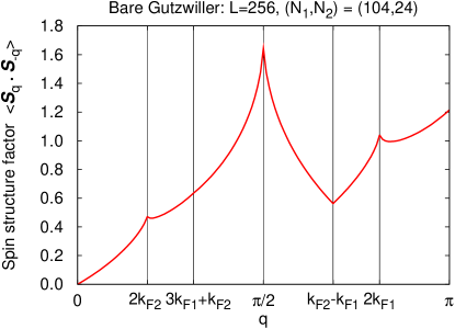
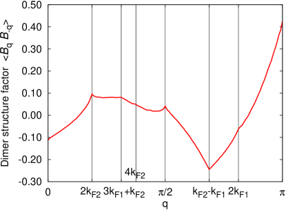
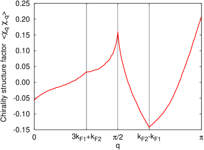
Figure 21: Spin, bond energy, and chirality structure factors in the bare Gutzwiller wavefunction with two Fermi seas $(N_{1},N_{2})=(104,24)$ on the 1D chain of length $L=256$. The expected singular wavevectors are marked by vertical lines (here $k_{F1}$ and $k_{F2}$ are defined as in Fig. 3 and all indicated wavevectors are modulo $2\pi$). The structure factors are symmetric with respect to $q\to-q$, and we only show $0\leq q\leq\pi$. The character of the singularities is consistent with the special case $g=1$ in the SBM theory of Sec. II.

The relative wavevectors connecting the Fermi points are gauge-independent and are observed in various quantities, see Fig. 21. Specifically, using variational Monte Carlo,Ceperley et al. (1977); Gros (1989) we measure the spin structure factor and see dominant singularities at the wavevectors $\pm 2k_{F1}$, $\pm 2k_{F2}$, and $\pm(k_{F1}+k_{F2})=\mp\pi/2$, which connect Fermi points with opposite group velocities. By studying sizes up to $L=512$ and performing scaling analysis at these wavevectors, the singularities appear to have the same power law. This is consistent only with the special case $g=1$ in the SBM theory [cf. Eqs. (80, 91) and Table 1]. Our direct estimates of the scaling dimensions are also consistent with the value $\Delta=3/4$ expected in this case. Turning to other less singular wavevectors, we clearly see V-shaped ($\sim|\delta q|$) features at $0$ and $\pi$ corresponding to scaling dimension $1$, which is expected generally. We also see $\pm(k_{F2}-k_{F1})$ with scaling dimension $1$, which requires $g=1$.

We next consider VBS correlations and see all of the above wavevectors, but we can not quantify the singularities as accurately. The VBS correlations also show singularities at $\pm(3k_{F1}+k_{F2})$ and $\pm 4k_{F2}=\mp 4k_{F1}$ (the former is also expected in the spin structure factor but is not visible there, probably due to amplitude effect, while the $\pm 4k_{F2}$ is expected only in the bond energy).

Finally, we measure spin chirality correlations and see dominant singularity at $\pm\pi/2$ consistent with $\Delta=3/4$. We also see singularities at wavevectors $0$, $\pi$, $\pm(k_{F2}-k_{F1})$, and $\pm(3k_{F1}+k_{F2})$ consistent with $\Delta=1$, again as expected in the special case $g=1$.

The above appears to hold for a range of relative populations of the Fermi seas (away from the limiting situations of a single or two equal Fermi seas). We are then led to conjecture that such spin-singlet wavefunctions with two Fermi seas have correlations given by the SBM theory of Sec. II and Appendix A with $g=1$. This conjecture is natural since in the theory the parameter $g$ depends on the ratio of the two Fermi velocities, cf. Eq. (21), while the wavefunction knows only about the occupied/unoccupied states and does not contain the band energy parameters. We leave proving this conjecture analytically as an open problem.

Given the preceding discussion, it appears that such bare Gutzwiller wavefunctions cannot capture fully the properties of the generic Spin Bose-Metal as described by the theory of Sec. II with general $g<1$. It is possible that they are appropriate wavefunctions for some critical end-points of the SBM phase where the parameter $g=1$, e.g., for the transitions out of the SBM discussed in Sec. IV.2. While the energetics study with the bare Gutzwiller wavefunctions gives us first indications for the SBM phase, it is desirable to have more accurate trial states. This is what we turn to next, although only with limited success.

B.2 SU(2)-invariant improvement of the Gutzwiller wavefunctions

To allow more variational freedom, we consider mean field with both spinon hopping $\xi(k)$, Eq. (3), and spinon pairing in the singlet channel with real gap function $\Delta(k)$ (this way, the wavefunction remains spin rotation and time reversal invariant). Generic $\Delta(k)$ would open up gaps, while we want the wavefunction to be critical. One way to maintain gaplessness is to require $\Delta(k)$ to vanish at the Fermi points. This can be achieved, for example, by taking

$$\Delta(k)=f(k)\xi(k)~{}$$ (110)

with a smooth $f(k)$. We have tried several simple functions $f(k)$, e.g., expanding in harmonics

$$f(k)=\sum_{n}f_{n}\cos(nk)~{},$$ (111)

with few $f_{n}$ treated as variational parameters. Upon writing out the corresponding Gutzwiller wavefunction, one can see that the dispersion $\xi(k)$ enters only through its sign $\xi<0$ or $\xi>0$, so in the case with two Fermi seas like in Fig. 20 we can use the same label $(N_{1},N_{2})$ and expect similar singular wavevectors encoded in the relative positions of the “Fermi points.” We refer to such a state as “improved Gutzwiller” and can view it as a “gapless superconductor,” although with caution because of the non-intuitive effects of the projection. For example, the SU(2) gauge structure of the projective construction implies that $f_{n}=A\delta_{n,0}$ gives the same state as the bare Gutzwiller independent of $A$. In practice, we often fix $f_{0}$ and vary $f_{1},f_{2}$.

For the zigzag ring model in the Spin Bose-Metal regime, such approach improves the trial energy by about 50-60% compared to the difference between the bare Gutzwiller energy and the exact DMRG ground state energy. The exponents of the power law correlations in the improved wavefunctions appear to remain unchanged from the bare case, although the numerical amplitudes are redistributed to resemble the DMRG correlations better, as can be seen in the examples in Sec. III.2, Figs. 4 and 5. Thus, this approach is only partially successful since we can not produce the long-distance behavior expected in the generic SBM and tentatively seen in the DMRG. Still, the fact that we can significantly improve the trial energy while retaining the underlying gapless character gives us more confidence in the variational identification of the SBM phase.

We also mention that in the Bethe-chain regime where the bare Gutzwiller projects one Fermi sea, the “gapless superconductor” improvement with parameters $f_{0},f_{2}$ works even better, bringing the trial energy much closer to the exact DMRG value and better reproducing short-scale features in the spin correlations, see Fig. 22. Such good trial states for the competing Bethe-chain phase give our VMC more accuracy in determining where the SBM phase wins energetically and more confidence interpreting the DMRG results.

B.3 States with fully polarized second Fermi sea

Motivated by the possibility of partial ferromagnetism in some regimes discovered in the DMRG study of the ring model (see in particular Sec. VI), we have also considered Gutzwiller projection of states with unpolarized large Fermi sea and fully polarized small Fermi sea. The spin correlations here can be understood using a naive Bosonization treatment starting with such spinon mean field state and following the same procedure as for the unpolarized Spin Bose-Metal in Sec. II. The naive long-wavelength theory now has two free Boson modes. The dominant correlations are expected to be at wavevectors that connect Fermi points with opposite group velocities. Taking the polarization axis to be $\hat{z}$, the spin structure factor $\langle S^{z}_{q}S^{z}_{-q}\rangle$ has dominant singularities at $2k_{F1}$, $2k_{F2}$, and $-k_{F2}-k_{F1}$, while the $\langle S^{x}_{q}S^{x}_{-q}\rangle$ is missing the $2k_{F2}$ since there is no spin-flip process across the second (polarized) Fermi sea. We indeed observe such correlations in the wavefunctions, and the dominant power law envelope is consistent with $x^{-4/3}$, which is what such naive theory would give if we assume equal velocities near all Fermi points and ignore all interactions other than gapping out the overall “charge” mode, Eq. (13). We note, however, that to properly describe such a partially polarized phase in the system with short-range interactions, we would need to also account for the ferromagnetic spin wave, which is not present in our wavefunctionsHaldane (1988) and not treated in the more general (but still naive) Bosonization theory outlined above. We do not pursue this further here.

Appendix C DMRG results in conventional phases on the zigzag chain

For ease of comparisons, here we show our DMRG measurements in the conventional Bethe-chain and VBS-2 phases identified on the zigzag chain in earlier works.White and Affleck (1996); Klironomos et al. (2007) We take representative points from the same cut $K_{\rm ring}/J_{1}=1$ studied in detail in Sec. III, since this allows us to better relate to the SBM phase at such significant $K_{\rm ring}$ values.

C.1 Bethe-chain phase

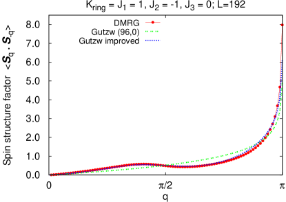
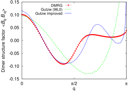
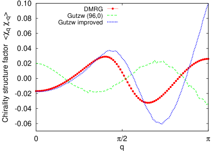
Figure 22: (Color online) Spin, dimer, and chirality structure factors at a representative point in the Bethe-chain phase, $K_{\rm ring}=J_{1}=1$, $J_{2}=-1$, measured in the DMRG for system size $L=192$. We also show structure factors in the bare Gutzwiller-projected single Fermi sea state, $(N_{1},N_{2})=(96,0)$, and in the improved Gutzwiller wavefunction with parameters $f_{0}=1,f_{1}=0,f_{2}=-1.4$ (see Appendix B for wavefunction details).

Figure 22 shows spin, dimer, and chirality structure factors at $J_{2}=-1$, measured in the DMRG for system size $L=192$. The DMRG can still obtain reliable results with $m=3200$ states kept in each block, and this is related to the smaller central charge than in the SBM phase (as discussed in Sec. III.4). Figure 22 also shows the structure factors in the bare Gutzwiller-projected single Fermi sea state, $(N_{1},N_{2})=(96,0)$, and in the improved Gutzwiller wavefunction (see Appendix B); the latter achieves significantly better trial energy and overall match with the DMRG results.

At long distances, we expect both the spin and dimer correlations to decay with the same power law: $\langle\vec{S}(x)\cdot\vec{S}(0)\rangle\sim(-1)^{x}/x$, $\langle{\cal B}(x){\cal B}(0)\rangle\sim(-1)^{x}/x$, up to logarithmic corrections. We indeed see roughly such power law in the real space correlations. Some quantitative aspects are different from the pure Heisenberg chain, for which the bare Gutzwiller state is a good approximation. Thus, the spin structure factor in Fig. 22 has a larger amplitude of the $q=\pi$ singularity and also develops a hump at wavevectors below $\pi/2$. Both these features are captured by the improved Gutzwiller wavefunction. On the other hand, the dimer structure factor has a significantly smaller amplitude of the $q=\pi$ singularity than the pure Heisenberg chain and the bare Gutzwiller; the improved Gutzwiller wavefunction moves in the right direction compared to the bare one but still does not capture well the amplitude at $\pi$.

For the chirality correlations, we expect $\langle\chi(x)\chi(0)\rangle\sim(-1)^{x}/x^{3}+1/x^{4}$, and we indeed see some fast decay in the real space data comparable with the power law behavior. The corresponding momentum space singularities at $q=\pi$ and $q=0$ are very weak. In agreement with this, we do not see any features in the chirality structure factor in Fig. 22.

This Bethe-chain phase example allows to contrast with the SBM phase in Sec. III.2, where we see different singular wavevectors and prominent features in all these observables including the chirality. The experience of being able to improve significantly the short-scale features in the trial wavefunctions carries over to the SBM, although in the Bethe-chain phase we have an advantage that our wavefunctions also capture the long-distance power laws correctly.

C.2 Valence Bond Solid with period 2

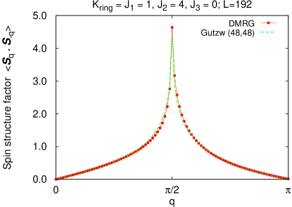
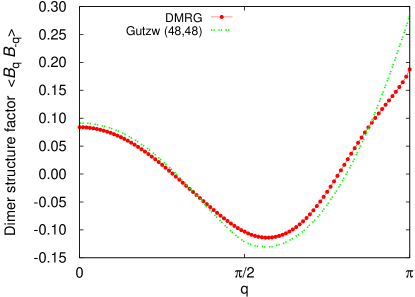
Figure 23: (Color online) Spin and dimer structure factors at a point in the VBS-2 phase, $K_{\rm ring}=J_{1}=1$, $J_{2}=4$, measured in the DMRG for system size $L=192$. The exhibited trial wavefunction is the Gutzwiller projection of two equal Fermi seas, $(N_{1},N_{2})=(48,48)$. This wavefunction gives decoupled legs expected in the large $J_{2}$ limit and does not have any VBS-2 order; however, it reproduces the DMRG data quite well, so at this $K_{\rm ring}=J_{1}$ cut the system is close to the decoupled legs limit even just outside the SBM.

Consider now the large $J_{2}$ case. In the $J_{2}\to\infty$ limit, we have decoupled legs, and each behaves as a Heisenberg spin chain. Finite $J_{1}/J_{2}$ and $K_{\rm ring}/J_{2}$ will couple the two legs and will likely open a spin gapWhite and Affleck (1996); Nersesyan et al. (1998) producing a VBS state with period 2 (Fig. 11). Figure 23 shows our measurements at a representative point $J_{2}=4$ from the $K_{\rm ring}=J_{1}=1$ cut. The spin correlations show a dominant peak at a wavevector $q=\pi/2$ and bond correlations have a peak at $q=\pi$. We compare with the Gutzwiller projection of two equal Fermi seas in the 1D zigzag chain language, or, equivalently, decoupled legs in the two-leg ladder picture. This wavefunction is thus strictly appropriate only in the $J_{2}\to\infty$ limit, but it clearly reproduces the DMRG data quite well.

Looking at Fig. 23, there is not much direct evidence for the VBS-2 order in the DMRG data. It is safe to say only that upon exiting the SBM phase along this cut, we are close to the fixed point of decoupled legs. One argument for the VBS-2 here could be the continuity to the strong VBS-2 phase in the broader phase diagram Fig. 2. As is known,White and Affleck (1996) the region $J_{2}\sim 0.4-2$ along the $K_{\rm ring}=0$ axis has strong VBS-2 order. However, this does not preclude possibility of more phases in the model with ring exchanges. Thus, along the way at points like $K_{\rm ring}=0.3,J_{2}=1.5$ and $K_{\rm ring}=0.2,J_{2}=1.2$ we also see a dimer feature at $q=\pi/2$ in addition to a likely Bragg peak at $q=\pi$. Since our primary interest is the SBM phase, we do not explore the states at large $J_{2}$ further, loosely referring to all of them as VBS-2 in Fig. 2.

References

- Shimizu et al. (2003) Y. Shimizu, K. Miyagawa, K. Kanoda, M. Maesato, and G. Saito, Phys. Rev. Lett. 91, 107001 (2003).
- Kurosaki et al. (2005) Y. Kurosaki, Y. Shimizu, K. Miyagawa, K. Kanoda, and G. Saito, Phys. Rev. Lett. 95, 177001 (2005).
- Yamashita et al. (2008) S. Yamashita, Y. Nakazawa, M. Oguni, Y. Oshima, H. Nojiri, Y. Shimizu, K. Miyagawa, and K. Kanoda, Nature Physics 4, 459 (2008).
- Yamashita et al. (2009) M. Yamashita, N. Nakata, Y. Kasahara, T. Sasaki, N. Yoneyama, N. Kobayashi, S. Fujimoto, T. Shibauchi, and Y. Matsuda, Nature Physics 5, 44 (2009).
- Motrunich (2005) O. I. Motrunich, Phys. Rev. B 72, 045105 (2005).
- Lee and Lee (2005) S.-S. Lee and P. A. Lee, Phys. Rev. Lett. 95, 036403 (2005).
- Senthil (2008) T. Senthil, Phys. Rev. B 78, 045109 (2008).
- McKenzie (1998, cond-mat/9802198) R. H. McKenzie, Comments Condens. Matter Phys. 18, 309 (1998, cond-mat/9802198).
- Morita et al. (2002) H. Morita, S. Watanabe, and M. Imada, J. Phys. Soc. Jpn. 71, 2109 (2002).
- LiMing et al. (2000) W. LiMing, G. Misguich, P. Sindzingre, and C. Lhuillier, Phys. Rev. B 62, 6372 (2000).
- Wen (2002, cond-mat/0107071) X.-G. Wen, Phys. Rev. B 65, 165113 (2002, cond-mat/0107071).
- Rantner and Wen (2002) W. Rantner and X.-G. Wen, Phys. Rev. B 66, 144501 (2002).
- Hermele et al. (2004) M. Hermele, T. Senthil, M. P. A. Fisher, P. A. Lee, N. Nagaosa, and X.-G. Wen, Phys. Rev. B 70, 214437 (2004).
- Lee et al. (2006) P. A. Lee, N. Nagaosa, and X.-G. Wen, Rev. Mod. Phys. 78, 17 (2006).
- Motrunich and Fisher (2007) O. I. Motrunich and M. P. A. Fisher, Phys. Rev. B 75, 235116 (2007).
- Sheng et al. (2008) D. N. Sheng, O. I. Motrunich, S. Trebst, E. Gull, and M. P. A. Fisher, Phys. Rev. B 78, 054520 (2008).
- Fisher et al. (arXiv:0812.2955) M. P. A. Fisher, O. I. Motrunich, and D. N. Sheng (arXiv:0812.2955).
- White and Affleck (1996) S. R. White and I. Affleck, Phys. Rev. B 54, 9862 (1996).
- Nersesyan et al. (1998) A. A. Nersesyan, A. O. Gogolin, and F. H. Esler, Phys. Rev. Lett. 81, 910 (1998).
- Klironomos et al. (2007) A. D. Klironomos, J. S. Meyer, T. Hikihara, and K. A. Matveev, Phys. Rev. B 76, 075302 (2007).
- Meyer and Matveev (2009) J. S. Meyer and K. A. Matveev, J. Phys. Cond. Matt. 21, 023203 (2009).
- Ioffe and Larkin (1989) L. B. Ioffe and A. I. Larkin, Phys. Rev. B 39, 8988 (1989).
- Holstein et al. (1973) T. Holstein, R. E. Norton, and P. Pincus, Phys. Rev. B 8, 2649 (1973).
- Reizer (1989) M. Reizer, Phys. Rev. B 40, 11571 (1989).
- Lee (1989) P. A. Lee, Phys. Rev. Lett. 63, 680 (1989).
- Lee and Nagaosa (1992) P. A. Lee and N. Nagaosa, Phys. Rev. B 46, 5621 (1992).
- Polchinski (1994) J. Polchinski, Nucl. Phys. B 422, 617 (1994).
- Altshuler et al. (1994) B. L. Altshuler, L. B. Ioffe, and A. J. Millis, Phys. Rev. B 50, 14048 (1994).
- Kim et al. (1994) Y. B. Kim, A. Furusaki, X. G. Wen, and P. A. Lee, Phys. Rev. B 50, 17917 (1994).
- Shankar (1995) R. Shankar, Acta Phys. Pol. B 26, 1835 (1995).
- Lin et al. (1998) H.-H. Lin, L. Balents, and M. P. A. Fisher, Phys. Rev. B 58, 1794 (1998).
- Fjaerestad and Marston (2002) J. O. Fjaerestad and J. B. Marston, Phys. Rev. B 65, 125106 (2002).
- Kim and Lee (1999) D. H. Kim and P. A. Lee, Ann. Phys. (N.Y.) 272, 130 (1999).
- Hosotani (1997) Y. Hosotani, J. Phys. A 30, L757 (1997).
- Mudry and Fradkin (1994) C. Mudry and E. Fradkin, Phys. Rev. B 50, 11409 (1994).
- White (1992) S. R. White, Phys. Rev. Lett. 69, 2863 (1992).
- White (1993) S. R. White, Phys. Rev. B 48, 10345 (1993).
- Schollwock (2005) U. Schollwock, Rev. Mod. Phys. 77, 259 (2005).
- Ceperley et al. (1977) D. M. Ceperley, G. V. Chester, and M. H. Kalos, Phys. Rev. B 16, 3081 (1977).
- Gros (1989) C. Gros, Annals Phys. (NY) 189, 53 (1989).
- Calabrese and Cardy (2004) P. Calabrese and J. Cardy, J. Stat. Mech. p. P06002 (2004).
- Haldane (1988) F. D. Haldane, Phys. Rev. Lett. 60, 635 (1988).
- Shastry (1988) B. S. Shastry, Phys. Rev. Lett. 60, 639 (1988).
- Matveev (2004a) K. A. Matveev, Phys. Rev. Lett. 92, 106801 (2004a).
- Matveev (2004b) K. A. Matveev, Phys. Rev. B 70, 245319 (2004b).
- Fiete (2007) G. A. Fiete, Rev. Mod. Phys. 79, 801 (2007).
- Daul and Noack (2000) S. Daul and R. M. Noack, Phys. Rev. B 61, 1646 (2000).
- Louis et al. (2001) K. Louis, J. V. Alvarez, and C. Gros, Phys. Rev. B 64, 113106 (2001).
- Capello et al. (2005) M. Capello, F. Becca, M. Fabrizio, S. Sorella, and E. Tosatti, Phys. Rev. Lett. 94, 026406 (2005).
- Japaridze et al. (2007) G. I. Japaridze, R. M. Noack, D. Baeriswyl, and L. Tincani, Phys. Rev. B 76, 115118 (2007).
- Singh et al. (1989) R. Singh, M. Fisher, and R. Shankar, Phys. Rev. B 39, 2562 (1989).
- Affleck et al. (1989) I. Affleck, D. Gepner, H. Schulz, and T. Ziman, J. Phys. A 22, 511 (1989).