Small Numbers of Vortices in Anisotropic Traps

Abstract

We investigate the appearance of vortices and vortex lattices in two-dimensional, anisotropic and rotating Bose-Einstein condensates. Once the anisotropy reaches a critical value, the positions of the vortex cores in the ground state are no longer given by an Abrikosov lattice geometry, but by a linear arrangement. Using a variational approach, we determine the critical stirring frequency for a single vortex as well as the equilibrium positions of a small number of vortices.

I Introduction

Quantized vortices are one of the hallmarks of superfluidity and the first observation of vortex lattices in liquid ⁴He Yarmchuk:79 , and more recently in gaseous Bose-Einstein condensates AboShaeer:01 , has lead to a large interest in studying their ground states and dynamical properties. Gaseous Bose-Einstein condensates are particularly well suited to the study of vortices, as their internal and external system parameters, such as the inter-atomic scattering length or the density, can be experimentally controlled. This allows access to study a large range of vortex states in different parameter regimes.

The structure of a ground state vortex lattice is given by the demand to minimise the energy of the system, under the condition of fixed angular momentum. For large angular momentum this is best done by forming an Abrikosov (triangular) lattice of charge one vortices AboShaeer:01 ; Anglin:02 . In different parameter regimes, however, other lattice structures have been shown to appear: symmetry preserving annular arrangements for small condensates Romanovsky:08 , rectangular lattices in traps with weak, superposed optical lattices Reijnders:04 , giant vortices in combined harmonic and quartic traps Aftalion:04 , and linear arrangements in atomic waveguide structures Sinha:05 .

While vortices are interesting from a fundamental point of view, it has recently been pointed out that the winding number of a single vortex can be engineered to create a topologically stable quantum bit for applications in quantum information Kapale:05 ; Thanvanthri:08 . Hallwood et al. have shown that to create proper macroscopic superposition states of angular momentum one needs to identify states which are close in energy, strongly coupling, and, at the same time, well separated from any other states Hallwood:07 . While these are difficult conditions to fulfill in gaseous Bose-Einstein condensates with short range interactions, the promise of long-lived qubits makes the effort worthwhile.

A second fundamental building block of quantum information processing is the ability to measure and control the interaction between two qubits. While interactions between vortices can be studied in Abrikosov lattices, it would be of advantage to find a geometry with a lower number of nearest neighbours. Two recent works have shown that systems where each vortex has only two nearest neighbours can be created in atomic waveguide structure Sinha:05 or in anisotropic, harmonic traps in the limit of weak interactions Oktel:04 .

Here we extend the two works above by considering a Bose-Einstein condensate deep in the non-linear regime (Thomas Fermi limit) and trapped in an anisotropic trap. By numerically determining the minimum energy state, we find that for relatively small aspect ratios, $\lambda\gtrapprox 2$, and moderate rotational frequencies the rotating Abrikosov lattice is no longer the ground state of the condensate and, instead, a linear crystal of vortices is formed along the soft axis of the trap. Taking advantage of the symmetry of the system, we devise an ansatz for a variational calculation in order to predict ground state properties of the system. We investigate the critical stirring frequencies needed to move from the $l=0$ to $l=1$ state and the locations in the lattice for a small number of vortices of equal rotational charge. Note that anisotropic traps in the strong rotation limit have recently been investigated in Aftalion:09 .

The paper is organised as follows. In Sec. II we introduce our variational wavefunction and calculate the energy of the system as a function of anisotropy. In Sec. III we determine the critical stirring frequencies for local and global stability of a single vortex in an anisotropic trap and in Sec. IV we calculate the ground state structure of a vortex crystal with a small number of vortices. In Sec. LABEL:sec:VortexDynamics we briefly discuss the dynamics of a linear vortex crystal in an anisotropic trap. In Sec. VI we conclude.

II Variational Calculation

II.1 Energy Functional

We consider a condensate of $N$ atoms with atomic mass $m$ and scattering length $a_{sc}$, trapped in a potential $U(\mathbf{r})$ that is rotating at frequency $\Omega$. The energy functional for such a system is given by

$$E[\Psi^{*},\Psi]= \int d^{2}\mathbf{r}\ dz\;\Psi^{*}\left[-\frac{\hbar^{2}}{2m}\nabla^{2}+U(\mathbf{r})-\mathbf{\Omega}\cdot\mathbf{L}\right]\Psi$$

$$+\frac{Ng_{3D}}{2}\int d^{2}\mathbf{r}\ dz\;|\Psi|^{4}\;,$$ (1)

where $\mathbf{L}$ is the angular momentum operator, $g_{3D}=4\pi\hbar^{2}a_{sc}/m$ is the coupling constant and $\int d^{3}\mathbf{r}\;|\Psi|^{2}=1$. Finding the equilibrium states for the above functional in all generality is a formidable task and beyond our analytical as well as numerical capabilities. We will, therefore, in the following make some assumptions on the symmetry of our system.

First, we will consider rotation around one of the major axes only. Therefore, by choosing the angular momentum operator to be $L_{z}$, we can separate the wave function into the $xy$-plane and the $z$-direction as $\Psi(x,y,z)=\psi(x,y)\phi(z)$. Since the contributions to the energy functional from the kinetic, potential and rotational energies from $\phi(z)$ are constant, we need only consider the contributions made to the coupling constant from the third dimension. In the following we will therefore make the assumption that the wave function in the $z$-direction is in the Thomas-Fermi limit and rescale the coupling constant as $g_{2D}=g_{3D}(m\omega_{z}/2\pi\hbar)^{1/2}$. This creates an effective, two-dimensional Hamiltonian to work with. Specifying the anisotropy of the harmonic trapping potential in the $xy$-plane by the parameter $\lambda$, we get the following energy functional

$$E[\psi^{*},\psi]= \int d^{2}\mathbf{r}\;\psi^{*}\Bigg{[}-\frac{\hbar^{2}}{2m}\nabla^{2}+\frac{m\omega^{2}}{2}\left(x^{2}+\lambda^{2}y^{2}\right)$$

$$\qquad\qquad\quad-\Omega L_{z}\Bigg{]}\psi$$

$$+\frac{Ng_{2D}}{2}\int d^{2}\mathbf{r}|\psi|^{4}\;.$$ (2)

II.2 Variational Ansatz

In order to find a good variational ansatz we need to consider both the effect the angular momentum has on the density of the condensate and the contribution to the phase of the condensate. A convenient and transparent way of doing this is to use the quantum hydrodynamic form and split the wavefunction into its modulus and phase Fetter:01

$$\psi(x,y)=|\psi|e^{iS}\;.$$ (3)

Considering the modulus first, we find that, in the Thomas-Fermi limit of large particle numbers, a condensate carrying vortices can be characterised by two length scales. The first is the overall condensate size and is given by the Thomas-Fermi radius Baym:96

$$R=\sqrt{\frac{2\mu}{m\omega^{2}}}\;,$$ (4)

where $\mu$ is the chemical potential of the system incluing the vortex lattice. The size of the vortex cores gives the second characteristic length scale. For an isotropic trap this is given by Castin:99

$$r_{core}\simeq\sqrt{\frac{\hbar^{2}}{m\mu}}\;.$$ (5)

and we will show later that this is still a valid expression in the anisotropic case. Since with increasing particle number these quantities are inversely proportional to each other, we can separate our ansatz with respect to these two scales as

$$\psi=\psi_{TF}\psi_{VL}\;.$$ (6)

The Thomas-Fermi part, $\psi_{TF}$, describes the background cloud and is given by the well known expression

$$\psi_{TF}=\left[\frac{1}{Ng}\left(\mu-\frac{m\omega^{2}}{2}(x^{2}+\lambda^{2}y^{2})\right)\right]^{\frac{1}{2}}\;.$$ (7)

The vortices are described by the function $\psi_{VL}$, which will only deviate from unity close to the individual vortex cores and for which we will use a product of $\tanh$ functions of variable width $\kappa=1/r_{core}$ Castin:99 . The full ansatz for the wave-function modulus therefore reads

$$|\psi|=\psi_{TF}\prod_{k=1}^{n}\tanh\left[\kappa|\vec{r}-\vec{a_{k}}R|\right]\;,$$ (8)

and describes $n$ vortices located at $\vec{a_{k}}$. Note that the vortex positions are scaled in units of the Thomas-Fermi radius in the soft direction $R$, which lets us restrict our values of $a_{k}$ to between $0$ (trap centre) and $1$ (condensate edge in the soft direction). We also define $\mu_{0}$ to be the chemical potential of a condensate with no vortices

$$\mu_{0}=\sqrt{\frac{m\omega^{2}Ng\lambda}{\pi}}\;.$$ (9)

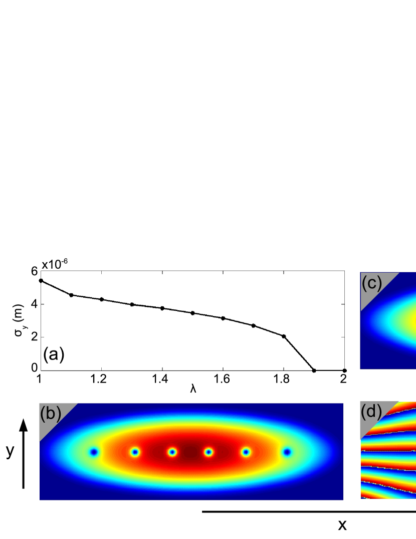
Figure 1: Numerical simulations for a ⁸⁷Rb gas of $N=10^{7}$ atoms with $a_{sc}=4.67\times~{}10^{-9}m$ and trapping frequency $\omega=20\pi s^{-1}$. (a) Standard deviation, $\sigma_{y}$, of the vortices from the x-axis for $1\leq\lambda\leq 2$. For $\lambda\geq 1.9$ the vortices form a linear crystal and $\sigma_{y}=0$. (b,c,d). Ground states for a condensate with parameters as above in a trap with aspect ratio of $\lambda=2.5$. Each plot spans a range of $-36\mu m<x<36\mu m$ and $-11\mu m<y<11\mu m$. (b) Ground state density for condensate rotating at $\Omega=0.7\omega$ showing 6 vortices. (c) Ground state density for condensate rotating at $\Omega=0.65\omega$ showing 5 vortices. (d) phase of the cloud shown in (c). The correspondence between the phase singularities and the density dips is indicated.

To further reduce the number of free variables in the energy functional, we will assume that we are in the anisotropic limit in which the vortices are forming a linear lattice Oktel:04 ; Sinha:05 . While this assumption at first glance looks only reasonable for extremely anisotropic systems where the Thomas-Fermi radius is of the order of the vortex core diameter, we have found through numerical simulations that linear crystals are already present for medium anisotropies if the number of vortices is small. This can be qualitatively understood by realising that the anisotropies lead to extended low density areas in the soft direction and an alignment along this axis therefore minimizes the vortex self energies as well as interactions. In Fig. 1(a) we show the standard deviation of the vortex core positions from $y=0$ for a system of 5 vortices as a function of anisotropy. For an isotropic trap the vortices form a triangular arrangement, which with increasing values of $\lambda$ becomes squeezed along the tight direction. For the relative moderate value of $\lambda=1.9$ the standard deviation $\sigma_{y}$ goes to zero and remains there for all higher values of anisotropy. Figs. 1(b)-(d) show these numerically determined ground states for an even and an odd number of vortices, illustrating this linear geometry. Therefore we assume that $\vec{a_{k}}=(a_{k},0)$, i.e. the vortices sit along the $x$-axis of the trap. Furthermore, due to the symmetry of the system, we can assume that for even numbers of vortices, vortex pairs are located at $(a_{k},0)$ and $(-a_{k},0)$ and for odd numbers of vortices, a single vortex will sit at the centre of the trap and the remaining vortices will pair off as in the even case.

Finally, the phase itself can be broken up into the phase of the condensate without vortices, $S_{0}$, and the phase from each vortex core of charge $q_{k}$

$$S(x,y)=S_{0}(x,y)+\sum_{k=1}^{n}q_{k}\theta_{k}\;.$$ (10)

The first part describes the phase of the anisotropic condensate under rotation without vortices and is given by Castin:99 ; Svidzinsky:00

$$S_{0}(x,y)=-\frac{m\Omega}{\hbar}\frac{\omega_{x}^{2}-\omega_{y}^{2}}{\omega_{x}^{2}+\omega_{y}^{2}}xy\;.$$ (11)

Since in our system the vortices are sitting along a single line along which the phase is constant, we can neglect this contribution to the phase and take

$$S=\sum_{k=1}^{n}q_{k}\theta_{k}.$$ (12)

II.3 Variational Energies

Having the defined the ansatz and energy functional in the last section, we can now calculate and minimise the different energies involved. All our results for single and two vortex systems match up with recent work by Castin and Dum Castin:99 in the isotropic limit.

II.3.1 Kinetic Energy

Since we assume our system to be in the Thomas-Fermi limit, we will neglect the spatial variation of the background condensate cloud when calculating the kinetic energy. We can then rewrite $\tanh^{2}(x)=1-\text{sech}^{2}(x)$ and take advantage of the fact that $\text{sech}^{2}(x)$ is non-zero only within a small distance from the vortex core. This allows us to neglect all terms that involve products of two different vortex cores, i.e. terms of the form $\text{sech}^{2}(x_{i})\text{sech}^{2}(x_{j}),(i\neq j)$ and leaves us the following expression for the kinetic energy Castin:99

$$E_{\text{kin}}= \frac{\hbar^{2}}{2m}\int d^{3}\mathbf{r}\;|\psi_{TF}|^{2}\sum_{k=1}^{n}\tanh^{2}\left[\kappa|\vec{r}-\vec{a_{k}}R|\right](\nabla\theta_{k})^{2}$$

$$+ \frac{\hbar^{2}}{2m}\int d^{3}\mathbf{r}\;|\psi_{TF}|^{2}\sum_{k=1}^{n}\kappa^{2}(\tanh\left[\kappa|\vec{r}-\vec{a_{k}}R|\right])^{2}$$

$$+ \frac{\hbar^{2}}{2m}\int d^{3}\mathbf{r}\;|\psi_{TF}|^{2}\sum_{k=1}^{n}\sum_{k^{\prime}\neq k}q_{k}q_{k^{\prime}}\nabla\theta_{k}\cdot\nabla\theta_{k^{\prime}}\;.$$ (13)

The first two terms describe contributions from single vortices and the last one accounts for the contributions from two vortices. As expected from our ansatz, the anisotropy is completely contained in the Thomas-Fermi parts. The single vortex terms can be straightforwardly integrated to give

$$E_{\text{kin}_{1}}= \sum_{k=1}^{n}\frac{\hbar^{2}\omega^{2}}{\mu_{0}}(1-a_{k}^{2})\left(\ln(\kappa^{2}R^{2})+\frac{1}{2}\ln(1-a_{k}^{2})-c\right)$$

$$-\sum_{k=1}^{n}\frac{\hbar^{2}\omega^{2}}{\mu_{0}}\frac{1-a_{k}^{2}(-5+\lambda)+\lambda}{2(1+\lambda)}\;,$$ (14)

where $c=(4\ln(2)-1)/6$ is a constant. The remaining term, $E_{\text{kin}_{2}}$, cannot be integrated analytically and we will solve it numerically when discussing interacting vortex systems below.

II.3.2 Potential and Rotational Energies

The potential and rotational energies are given by

$$E_{\text{pot}}= \sum_{k=1}^{n}\int d^{2}\mathbf{r}\;|\psi|^{2}\left[\frac{m\omega^{2}}{2}(x^{2}+\lambda^{2}y^{2})+\frac{Ng}{2}|\psi|^{2}\right]\;,$$ (15)

$$E_{\text{rot}}= -\sum_{k=1}^{n}\hbar\Omega\int d^{2}\mathbf{r}\;|\psi_{TF}|^{2}\left(x\frac{\partial}{\partial y}-y\frac{\partial}{\partial x}\right)q_{k}\theta_{k}\;,$$ (16)

and can be integrated to give

$$E_{\text{pot}}= \sum_{k=1}^{n}2\mu_{0}c\frac{(1-a_{k}^{2})}{\kappa^{2}R^{2}}\;,$$ (17)

$$E_{\text{rot}}= -\sum_{k=1}^{n}\frac{q\hbar\Omega}{2}\frac{\lambda^{2}(3-4a_{k}^{2})-1}{\lambda^{3}}\;.$$ (18)

To be able to calculate the rotational integral we have made one further approximation by considering only the area traced out by a circle around the vortex whose radius is the same size as the trap in the tight direction. This means that we only take into account the cylindrically symmetric contribution to the phase close to the vortex and neglect the asymmetric contributions from the low-density edges of the cloud Svidzinsky:00 .

The total energy of the system can now be expressed as

$$E=\frac{2\mu_{0}}{3}+\sum_{k=1}^{n}W(a_{k})+\sum_{k=1}^{n}\sum_{k^{\prime}>k}^{n}I(a_{k},a_{k^{\prime}})\;,$$ (19)

where the single vortex self energy is given by

$$W(a)= E_{\text{kin}_{1}}+E_{\text{pot}}+E_{\text{rot}}$$

$$= \frac{\hbar^{2}\omega^{2}}{\mu_{0}}(1-a^{2})\left(\ln(\kappa^{2}R^{2})+\frac{1}{2}\ln(1-a^{2})-c\right)$$

$$-\frac{\hbar^{2}\omega^{2}}{\mu_{0}}\frac{1-a^{2}(\lambda-5)+\lambda}{2(1+\lambda)}$$

$$+2\mu_{0}c\frac{(1-a^{2})}{\kappa^{2}R^{2}}$$

$$+\frac{q\hbar\Omega}{2}\frac{1-\lambda^{2}(3-4a^{2})}{\lambda^{3}}\;,$$ (20)

and the interaction between two vortices of identical charge $q_{k}=q_{k^{\prime}}=\pm 1(k\neq k^{\prime})$ can be found from

$$I(a_{k},a_{k^{\prime}})=E_{\text{kin}_{2}}=\frac{\hbar^{2}}{2m}\int d^{2}\mathbf{r}\;|\psi_{TF}|^{2}\nabla\theta_{\vec{a_{k}}}\cdot\nabla\theta_{\vec{a_{k^{\prime}}}}\;.$$ (21)

III Critical Stirring Frequency for a Single Vortex

Let us first consider the critical frequency for a single vortex state to become the stable ground state of the trap. Two factors have to be taken into account, namely the existence of two different trapping frequencies and the fact that the lower one sets an upper limit for rotational stability in a harmonic potential. To study the physics of a single vortex, we need only consider the vortex self energy, $W$. We therefore minimise eq. (II.3.2) first with respect to $\kappa$ and find that the size of a vortex core is related only to the chemical potential of the cloud at the site of the vortex Castin:99

$$(\kappa R)^{2}=4c(1-a^{2})\frac{\mu_{0}^{2}}{\hbar^{2}\omega^{2}}\;.$$ (22)

In particular we note that this expression is independent of the strength of the anisotropy which justifies our earlier assumption that we can separate two length scales in the system. Using eq. (22) we can then express the self energy as

$$W= \frac{\hbar^{2}\omega^{2}}{\mu_{0}}(1-a^{2})\left(\ln\left(\frac{2\sqrt{c}\mu_{0}}{\hbar\omega}\right)+\frac{1}{2}\ln(1-a^{2})+c\right)$$

$$+\frac{\hbar^{2}\omega^{2}}{\mu_{0}}\left(3a^{2}(\lambda^{2}-5)-\frac{3a^{2}}{1+\lambda}\right)$$

$$+\frac{q\hbar\Omega}{2}\frac{1-\lambda^{2}(3-4a^{2})}{\lambda^{3}}$$ (23)

where again the first line corresponds to the kinetic energy, the second corresponds to the potential energy, the third corresponds to the rotational energy. From this expression for the energy, we can derive the two critical stirring frequencies, $\Omega_{l}$ and $\Omega_{g}$, corresponding to the appearance of a local and global energy minimum, respectively.

The local minimum corresponds to the point where $W$ changes from having a local maximum to a local minimum at the centre of the trap and is found by setting $\partial_{a}^{2}W=0$ at $a=0$

$$\Omega_{l}=\frac{\hbar\omega^{2}}{\mu_{0}}\frac{2\lambda^{3}}{3\lambda^{2}-1}\ln\left(\frac{C\mu_{0}}{\hbar\omega}\right)\;,$$ (24)

where $C=2\sqrt{c}e^{c}$. For this value of the stirring frequency a vortex becomes locally stable in the condensate.

The global minimum is the frequency for which which the energy of the condensate with a vortex at the centre has lower energy than the condensate without the vortex, i.e. $W=0$ at $a=0$

$$\Omega_{g}=\frac{\hbar\omega^{2}}{\mu_{0}}\frac{\lambda}{2}\left[\frac{4+\lambda}{1+\lambda}+\ln\left(\frac{C\mu_{0}}{\hbar\omega}\right)\right]\;.$$ (25)

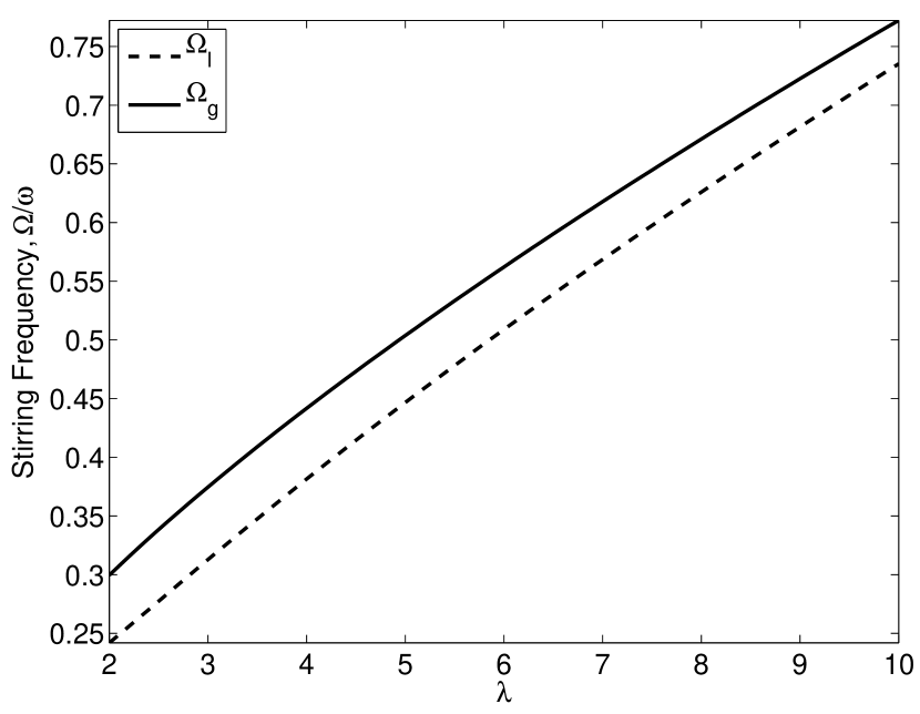
Figure 2: Critical frequency for a single vortex as a function of aspect ratio, $\lambda$. Stirring frequencies are defined in terms of the trapping frequency in the soft direction, $\omega$. For stirring frequencies greater than $\omega$, the cloud becomes unstable. $N=1\times~{}10^{5}$, $\omega=20\pi s^{-1}$, and $a_{sc}=4.67\times~{}10^{-9}m$ is the s-wave scattering lenghth for Rubidium-87.

Both quantities are shown in Fig. 2 as a function of anisotropy. One can see that both expressions above are not simple extensions of the isotropic version, as they do not scale linearly with $\lambda$. This agrees with earlier results showing the appearance of irrotational velocity fields in rotating anisotropic traps before vortex nucleation Svidzinsky:00 .

IV Equilibrium lattice positions

In the following we will calculate the equilibrium positions of small numbers of vortices in anisotropic traps as a function of anisotropy. While for symmetry reasons a stable single vortex will sit in the centre of the harmonic trap, the positions of larger numbers of vortices are determined by a complex interplay between the single vortex energies of eq. (II.3.2), and the vortex-vortex interactions given by eq. (21). As argued above, we will assume that the vortices are arranged in a linear crystal which is aligned along the $x$-axis and symmetric with respect to the $y$-axis of the trap.

For two vortices of equal charge and located at $\pm a$ the integral for the vortex-vortex interaction, eq. (21), can be explicitly written out as

$$I=\frac{\hbar^{2}}{2m}\int d^{2}\mathbf{r}\;|\psi_{TF}|^{2}\frac{x^{2}+y^{2}-a^{2}}{\left((x-a)^{2}+y^{2}\right)\left((x+a)^{2}+y^{2}\right)}\;.$$ (26)

This expression cannot be fully integrated analytically and we therefore minimise the complete energy functional numerical with respect to the vortex positions $\pm a$. The results are shown for different rotational frequencies in Fig. 3 as a a function of anisotropy. The regions in which the two-vortex molecule is the stable ground state of the system are marked by the black parts of the curve. As the above minimisation procedure does not give any information about the stability of the system, we have determined these areas through numerical ground state calculations. Note that they are only indicative though, since pinning down exact borders is a challenging numerical task beyond our capabilities. Also note that we display real units here, since the Thomas-Fermi radius changes as a function of the rotation frequency.

The first thing one can see from Fig. 3 is that with increasing anisotropy the vortices are moving away from the trap centre. This behaviour is a reaction to the increased non-linearities due to the tighter potential in the transversal direction, which has the effect of higher single vortex energies as well as vortex-vortex interactions. Increasing the rotation frequency has the opposite effect, as one can see from the relative position of the three curves displayed. Faster rotation, i.e. larger $\Omega$, leads to an increased Thomas-Fermi radius in the soft direction and allows for lower densities near the centre. The vortices therefore move back towards the centre. The detailed form of this behaviour for continuous $\Omega$ is shown in Fig. 4.

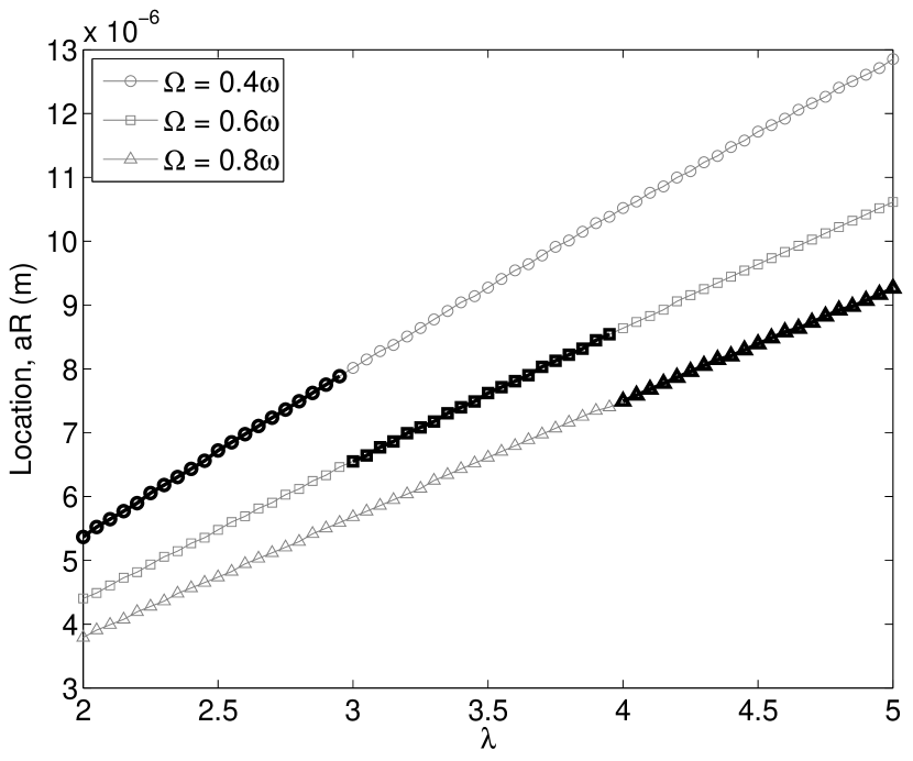
Figure 3: Distance of each vortex in a vortex pair from the centre of the trap as a function of aspect ratio. The results are shown for a gas of $N=1\times~{}10^{5}$ atoms of ⁸⁷Rb. The trapping frequency is given by $\omega=20\pi s^{-1}$ and we display three different rotational frequencies $\Omega=0.4\omega,0.6\omega$ and $0.8\omega$. The regions in which the two-vortex state is stable is marked by the black part of the graphs.

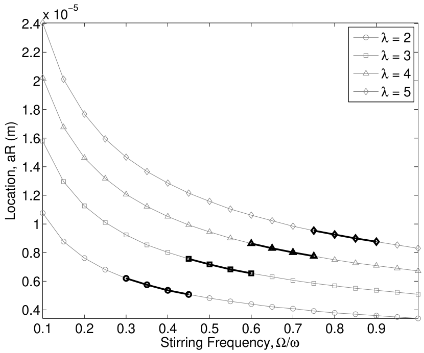
Figure 4: Distance of each vortex in a vortex pair from the centre of the trap as a function of the stirring frequency. The system parameters are the same as in Fig. 3 and we display four different aspect ratios. The stable regions are again the parts marked by the black lines.

For the three vortex case we again use the symmetry argument to choose an ansatz in which the central vortex is located at $(0,0)$ and the other vortices are located at $(\pm a,0)$. We now have include the interaction between all three vortices, giving us three integrals, two of which will be identical due to the symmetry. Fig. 5 shows the location of the outer vortices as a function of the aspect ratio. As with the two vortex case, the vortices settle further away from the centre the more anisotropic the trap is, however the distance is larger than in the previous case. This is clearly due to the addition of the repulsive centre vortex and when comparing the two and three vortex case, one can see that the distance from the centre is about doubled. This indicates that for at least small numbers of vortices within the TF cloud the distance between two vortices is almost constant and which confirms the overall trend that can be seen from the simulations shown in Fig. 1. This behaviour is also known from the two-dimensional Abrikosov lattices Anglin:02 . Again, as in the two vortex case and for the same reason, the vortices moves inward with increasing trapping frequency (see Fig. 6).

It is easy to see how this method can be expanded for larger numbers of vortices, taking advantage of the symmetry of the system. However, the number of interaction terms required for $N$ vortices is $N(N-1)/2$ requiring increased computational power and time.

Figure 5: Distance of outer vortices from central vortex in the three vortex case as a function of anisotropy for a range of stirring frequencies. The system parameters are the same as in the two vortex case.

Figure 6: Distance of outer vortices from central vortex in the three vortex case as a function of the stirring frequency for a range of anisotropies. The system parameters are the same as in the two vortex case.

V Vortex Dynamics

While the above determines the ground state of the condensate, it does not guarantee that the dynamical evolution maintains the linear shape of the vortex crystal over time. In fact, the force on a vortex in an inhomogeneous potential is directed perpendicular to the gradient of the potential and one can therefore expect movement of each vortex along an equipotential line of the trap. While in an isotropic trap this would lead to a simple rotation of the linear crystal around the centre of the trap, in an anisotropic trap this leads to a change in relative distance between two vortices. Shorter distances, however, mean larger repulsive forces and one can see that beyond a critical anisotropy the vortices will be unable to pass each other along the perpendicular direction and will therefore maintain the linear crystal structure.

While the dynamical evolution is not the topic of the current work, we have confirmed the above intuition by simulating the dynamical behaviour of our system for a wide range of parameters and anisotropies. In Fig. 7 we show the trajectories of five vortex cores in a trap with an anisotropy parameter of $\lambda=2.5$ for a duration of $t=3.5$s. One can see that the vortices move around in the vicinity of their original position, however they are not able to pass each other out. In fact, the linear shape of the vortex crystal is maintained at any time and we do not even observe any bending. At some point, for even longer timescales, the backaction of the vortex movement will lead to excitations of the background density and an exchange in vortex position might happen. This will be the investigation of a future work.

Figure 7: Trajectories of the single vortices over a time interval of $t=3.5$s. One can see that the outer vortices move around their equilibrium positions (white dots), but do not pass each other out. The central vortex remains stationary throughout. The system parameters are the same as in the figures above.

VI Conclusion

Our work fills the gap between two recent investigations into vortex lattice structures in anisotropic traps, one in the low density limit Oktel:04 and the other in the fast rotational limit Aftalion:09 . We have shown numerically that a small change in the anisotropy of a moderately rotating anisotropic Bose-Einstein condensate in the Thomas-Fermi limit changes the geometry of vortex lattice from hexagonal to linear and we have presented a variational analysis of such a system. Using the simple symmetry of the linear geometry we have devised a straightforward ansatz in the Thomas-Fermi limit, which allowed us to split the energy function into single vortex terms and two vortex interaction terms. From this we have been able to determine the critical frequency for the creation of a single vortex and found that as the aspect ratio increases, the critical stirring frequency increases.

Minimising the energy functional for two and three vortex state, we were able to determine the exact positions of the vortex cores. This is a very tedious exercise for direct numerical treatments, as many vortex lattices configurations have energies closely related to each other. We found that the distance of the vortices from the centre increases with increasing aspect ratio, however, it decreases as the stirring frequency increases. At least for systems with small numbers of vortices we found that the distance between neighbouring cores is effectively constant.

Finally we briefly addressed the dynamical behaviour of a linear vortex crystal and showed that for sufficiently anisotropic traps the linear crystal geometry is maintained for very long time-scales.

- (1) E.J. Yarmchuk, M.J.V. Gordon, R.E. Packard, Phys. Rev. Lett. 43, 214 (1979) .
- (2) J.R. Abo-Shaeer, C. Raman, J.M. Vogels, W. Ketterle, Science 292, 476 (2001).
- (3) J.R. Anglin, M. Crescimanno, arXiv:cond-mat/0210063v1 (2002).
- (4) I. Romanovsky, C. Yannouleas, U. Landman, Phys. Rev. A 78, 011606(R) (2008).
- (5) J.W. Reijnders and R.A. Duine, Phys. Rev. Lett. 93, 060401 (2004).
- (6) A. Aftalion and I. Danaila, Phys. Rev. A 69, 033608 (2004).
- (7) Y. Shin, M. Saba, M. Vengalattore, T.A. Pasquini, C. Sanner, A.E. Leanhardt, M. Prentiss, D.E. Pritchard, and W. Ketterle, Phys. Rev. Lett. 93, 160406 (2004).
- (8) S. Sinha and G.V. Shlyapnikov, Phys. Rev. Lett. 94, 150401 (2005).
- (9) K.T. Kapale and J.P. Dowling, Phys. Rev. Lett. 95, 173601 (2005).
- (10) S. Thanvanthri, K.T. Kapale, J.P. Dowling, Phys. Rev. A 77, 053825 (2008).
- (11) D.W. Hallwood, K. Burnett, and J. Dunningham, J. Mod. Opt. 54, 2129 (2007).
- (12) M.Ö. Oktel, Phys. Rev. A 69, 023618 (2004).
- (13) A. Aftalion, X. Blanc, and N. Lerner, Phys. Rev. A 79, 011603 (2009).
- (14) A.L. Fetter and A.A. Svidzinsky, J. Phys.: Condens. Matter 13, R135 (2001).
- (15) G. Baym and C.J. Pethick, Phys. Rev. Lett. 76, 6 (1996).
- (16) Y. Castin and R. Dum, Eur. Phys. J. D 7, 399 (1999).
- (17) A.A. Svidzinsky and A.L. Fetter, Physica B 284, 21 (2000).
- (18) K. W. Madison, F. Chevy, W. Wohlleben, and J. Dalibard, Jour. Mod. Optics 47, 2715 (2000)