Periodic travelling waves in convex Klein-Gordon chains

Abstract

We study Klein-Gordon chains with attractive nearest neighbour forces and convex on-site potential, and show that there exists a two-parameter family of periodic travelling waves (wave trains) with unimodal and even profile functions. Our existence proof is based on a saddle-point problem with constraints and exploits the invariance properties of an improvement operator. Finally, we discuss the numerical computation of wave trains.

Keywords:

Klein-Gordon chain, lattice travelling waves, constrained optimisation

MSC (2000):

37K60, 47J30, 70F45, 74J30

1 Introduction

Chains of coupled particles or oscillators have a broad range of applications in physics, material science, and biology, see for instance [DPB93, BK04], and have been studied intensively during the last decades. For chains of identical particles coupled by nearest neighbour interactions the law of motion reads

$$m\ddot{y}_{j}+{\gamma}\dot{y}_{j}=\Phi^{\prime}{\left({y_{j+1}-y_{j}}\right)}-\Phi^{\prime}{\left({y_{j}-y_{j-1}}\right)}-\Psi^{\prime}{\left({y_{j}}\right)}.$$ (1)

Here $y_{j}{\left({t}\right)}$ is the displacement of the $j$th particle at time $t$, $m$ the particle mass, ${\gamma}\geq 0$ a damping parameter, and $\Phi$ and $\Psi$ denote the pair and on-site potential, respectively. Examples for such chains with ${\gamma}=0$ are FPU-like chains with $\Psi\equiv 0$, and Klein-Gordon chains with arbitrary on-site but harmonic pair potential. Moreover, in the case $\Psi{\left({y}\right)}=\sin{y}$ one either refers to (1) as the Frenkel-Kontorova model or the discrete Sine-Gordon equation.

Major topics in the analysis of atomic chains like (1) are the existence and dynamical properties of coherent structures such as travelling waves and breathers, see the review article [IJ05]. A travelling wave is a special solution to (1) which satisfies

$$y_{j}{\left({t}\right)}=Y{\left({kj-{\omega}{t}}\right)},$$ (2)

where $k$ and ${\omega}$ denote the wave number and frequency, respectively, and $Y$ is the profile function.

The existence of travelling wave solutions to (1) has been investigated by several authors using rather different methods. For chains with harmonic $\Phi$ we refer to [IK00] which establishes the existence of small amplitude waves by using spatial dynamics and centre manifold reduction, see also [IP06]. Numerical simulations are presented in [DEFW93], and [MJKA02] investigates the existence and stability of standing waves by using a continuum approximation for the small amplitude limit. More recently, the existence of periodic travelling waves for the Frenkel-Kontorova model was shown in [Kat05] by means of fixed point methods, and [BZ06] provides existence results in Sine-Gordon chains with even non-local interactions. Close to our approach are [KZ08b, KZ08a], which set the problems also in a variational framework and prove the existence of supersonic waves for Sine-Gordon chains. Finally, a lot of literature addresses the existence of travelling waves in FPU-like chains, compare [Pan05, IJ05, Her08] and references therein.

In this paper we restrict ourselves to Klein-Gordon chains with convex on-site potential $\Psi$ and attractive nearest neighbour forces, and consider periodic travelling waves, which in turn are called wave trains. Due to simple normalisations we can suppose that $m=1$ and $\Phi{\left({y}\right)}=\tfrac{1}{2}y^{2}$, so the profile of each wave train must solve the nonlinear advance-delay differential equation

$$\omega^{2}{}\frac{\,\mathrm{d}^{2}}{\,\mathrm{d}{\varphi}^{2}}Y=\triangle_{k}{Y}-\Psi^{\prime}{\left({Y}\right)},$$ (3)

where ${\varphi}=kj-{\omega}{t}$ abbreviates the phase, and $\triangle_{k}$ is a discrete Laplacian with

$${\left({\triangle_{k}{Y}}\right)}{\left({{\varphi}}\right)}=Y{\left({{\varphi}+k}\right)}+Y{\left({{\varphi}-k}\right)}-2Y{\left({{\varphi}}\right)}.$$ (4)

Moreover, since (3) is invariant under shifts in ${\varphi}$-direction and under the scaling

$$Y{\left({{\varphi}}\right)}\rightsquigarrow Y{\left({{\lambda}{\varphi}}\right)},\qquad k\rightsquigarrow{\lambda}^{-1}k,\qquad{\omega}\rightsquigarrow{\lambda}^{-1}{\omega},$$

we can assume that $Y$ is $1$-periodic with unit cell ${\Lambda}=[-1/2,\,1/2)$.

In order to proof the existence of $1$-periodic solutions to (3) we follow a variational approach and characterise wave trains as solutions to a constraint saddle point problem for the potential energy. In particular, the frequency ${\omega}$ turns out to be the square root of the Lagrange multiplier, and cannot be prescribed. This is different from the standard variational method which prescribes the frequency and characterises travelling waves as stationary points of the action integral, compare for instance [KZ08b, KZ08a].

A further key ingredient for our method is an improvement operator, which we introduce below. Due to the convexity of $\Psi$ this operator possesses nontrivial invariant cones, and this allows to establish the existence of wave trains within these cones. More precisely, our main result can be stated as follows.

Theorem 1.

There exists a two-parameter family of solutions to (3) such that the profile function $Y$ is $1$-periodic, unimodal, and even.

The paper is organised as follows. In §2 we describe our variational setting, and §3 contains the proof of the main result. Finally, in §4 we discuss the numerical approximation of wave trains and present some simulations.

2 Variational setting

In the remainder of this paper we rely on the following standing assumption.

Assumption 2.

The on-site potential $\Psi:{\mathbb{R}}\to{\mathbb{R}}$ is twice continuously differentiable and uniformly convex, in the sense that there exist two constants $0<m<M<\infty$ such that $m\leq\Phi^{\prime\prime}{\left({x}\right)}\leq{M}$ for all $x\in{\mathbb{R}}$. Moreover, $\Psi$ is always normalised by $\Psi{\left({0}\right)}=\Psi^{\prime}{\left({0}\right)}=0$.

This assumption in particular implies

$$\tfrac{1}{2}mx^{2}\leq\Psi{\left({x}\right)}\leq\tfrac{1}{2}Mx^{2},\qquad\left|{\Psi^{\prime}{\left({x}\right)}}\right|\leq{M}\left|{x}\right|$$

for all $x\in{\mathbb{R}}$, and that $\Psi$ has a unique global minimum at $x=0$. We mention that the proofs below require $m$ and $M$ to exist only for all bounded sets, so our results remain valid if $\Phi^{\prime\prime}$ is bounded and uniformly positive on each closed interval.

Spaces and cones of functions

We denote by ${\mathsf{C}}^{k}$ the space of all functions that are periodic with unit cell ${\Lambda}$ and $k$ times continuously differentiable, and equip these spaces with their usual norms. Similarly, ${\mathsf{L}}^{2}$ is the space of all periodic functions which are square integrable on ${\Lambda}$, and ${\mathsf{H}}^{1}$ abbreviates the space of all functions $Y\in{\mathsf{L}}^{2}$ which have a weak derivative $Y^{\prime}\in{\mathsf{L}}^{2}$. Both ${\mathsf{L}}^{2}$ and ${\mathsf{H}}^{1}$ are Hilbert spaces with scalar products

$${\left\langle{Y_{1}},\,{Y_{2}}\right\rangle}_{{\mathsf{L}}^{2}} =\int_{{\Lambda}}{Y_{1}}{\left({{\varphi}}\right)}{Y_{2}}{\left({{\varphi}}\right)}\,\mathrm{d}{\varphi},\qquad{\left\langle{Y_{1}},\,{Y_{2}}\right\rangle}_{{\mathsf{H}}^{1}}={\left\langle{Y_{1}^{\prime}},\,{Y_{2}^{\prime}}\right\rangle}_{{\mathsf{L}}^{2}}+\int_{{\Lambda}}{Y_{1}}{\left({{\varphi}}\right)}\,\mathrm{d}{\varphi}\int_{{\Lambda}}{Y_{2}}{\left({{\varphi}}\right)}\,\mathrm{d}{\varphi}.$$

Note that ${\left\langle{\cdot},\,{\cdot}\right\rangle}_{{\mathsf{H}}^{1}}$ is equivalent to the standard scalar product as $Y\mapsto\left|{\int_{{\Lambda}}Y{\left({{\varphi}}\right)}\,\mathrm{d}{\varphi}}\right|$ defines a norm for the constants. Finally, we denote by ${\mathsf{H}}^{1}_{0}$ the closed subspace of all functions $X\in{\mathsf{H}}^{1}$ with $\int_{{\Lambda}}{X}{\left({{\varphi}}\right)}\,\mathrm{d}{\varphi}=0$, and set

$$\mathcal{B}_{\gamma}:=\left\{X\in{\mathsf{H}}^{1}_{0}\;:\;\tfrac{1}{2}{\|{X^{\prime}}\|}_{2}^{2}\leq{\gamma}\right\}.$$

To characterise the qualitative properties of wave trains we introduce the cone $\mathcal{U}$ of all unimodal and even functions on ${\Lambda}$, that is

$$\mathcal{U} {:=}\left\{Y\in{\mathsf{C}}^{0}\;:\;Y{\left({-{\varphi}}\right)}=Y{\left({{\varphi}}\right)}\;\text{and}\;Y{\left({\tilde{{\varphi}}}\right)}\geq{Y}{\left({{\varphi}}\right)}\;\text{for all}\;0\leq\tilde{{\varphi}}\leq{\varphi}\leq\tfrac{1}{2}\right\},$$

and define a further cone $\mathcal{C}$ by

$$\mathcal{C}{:=}\left\{Y\in{\mathsf{C}}^{2}\;:\;-Y^{\prime\prime}\in\mathcal{U}\right\}.$$

By construction, we have $Y\in\mathcal{U}$ if and only if $-Y{\left({\tfrac{1}{2}+\cdot}\right)}\in\mathcal{U}$, and below in Lemma 13 we show that $\mathcal{C}$ is a subcone of $\mathcal{U}$.

Examples of wave trains

We proceed with some explicit solutions to the wave train equation (3).

Remark 3.

For $k=0$ the wave train equation reduces to the oscillator ODE

$$\omega^{2}{}Y^{\prime\prime}=-\Psi^{\prime}{\left({Y}\right)}.$$ (5)

Therefore, there exists a one-parameter family of wave trains with $Y\in\mathcal{C}$, which can be parametrised by the energy $E=\tfrac{1}{2}{\omega}^{2}{Y^{\prime}}^{2}+\Psi{\left({Y}\right)}$.

Proof.

For given $E>0$ we pick $y<0$ such that $\Psi{\left({y}\right)}=E$ and define the function ${\widetilde{Y}}={\widetilde{Y}}{\left({t}\right)}$ with $t\in{\mathbb{R}}$ as solution to ${\widetilde{Y}}^{\prime\prime}{\left({t}\right)}=-\Psi{\big{(}{\widetilde{Y}}{\left({t}\right)}\big{)}}$ with initial conditions ${\widetilde{Y}}{\left({0}\right)}=y$ and ${\widetilde{Y}}^{\prime}{\left({0}\right)}=0$. According to the properties of $\Psi$, compare Assumption 2, this function ${\widetilde{Y}}$ is periodic with period $T=T{\left({E}\right)}$, satisfies ${\widetilde{Y}}{\left({t}\right)}={\widetilde{Y}}{\left({T-t}\right)}$, and is strictly increasing on $[0,\,T/2]$. We now define $Y\in\mathcal{U}$ by $Y{\left({{\varphi}}\right)}={\widetilde{Y}}{\big{(}T{\varphi}+T/2\big{)}}$, which solves (5) with ${\omega}=1/T$. ∎

Remark 4.

For the harmonic potential $\Psi{\left({x}\right)}=\tfrac{c}{2}{x}^{2}$ there exists a two-parameter family of wave trains with $Y\in\mathcal{C}$ given by

$${Y}{\left({{\varphi}}\right)}=a\cos{\left({2\pi{\varphi}}\right)},\quad{\omega}^{2}=\frac{4\sin{\left({k\pi}\right)}^{2}+c}{4\pi^{2}},$$ (6)

where the wave number $k$ and the amplitude $a>0$ are the free parameters.

Proof.

We introduce the Fourier transform ${\left({y_{m}}\right)}_{m\in{\mathbb{Z}}}$ of $Y$, that means

$$Y{\left({{\varphi}}\right)}=\sum\limits_{m\in{\mathbb{Z}}}y_{m}{{\mathtt{e}}^{\mathtt{i}2\pi{m}{\varphi}}},\qquad y_{m}=\int_{{\Lambda}}Y{\left({{\varphi}}\right)}{{\mathtt{e}}^{-\mathtt{i}2\pi{m}{\varphi}}}\,\mathrm{d}{\varphi},$$

and find (3) to be equivalent to

$$4\pi^{2}m^{2}\omega^{2}{}y_{m}={\left({2{\left({1-\cos{\left({2\pi{mk}}\right)}}\right)}+c}\right)}y_{m},\quad{m}\in{\mathbb{Z}}.$$

To solve this we set $y_{m}=y_{-m}=\tfrac{1}{2}\,\delta_{m}^{1}$, with $\delta_{m}^{1}$ being the Kronecker delta, and thanks to $1-\cos{2z}=2\sin^{2}{z}$ we obtain (6). ∎

The Lagrangian structure

For general $\Psi$ and $k\neq 0$ we cannot solve the wave train equation explicitly but need more sophisticated arguments to prove the existence of solutions. The starting point for each variational approach is the Lagrangian of a wave train

$$\mathcal{L}{\left({Y}\right)}={\omega}^{2}{\Gamma}{\left({Y}\right)}-\mathcal{P}_{k}{\left({Y}\right)},\qquad{\Gamma}{\left({Y}\right)}=\tfrac{1}{2}\int_{{\Lambda}}{Y}^{\prime}{\left({{\varphi}}\right)}^{2}\,\mathrm{d}{\varphi},$$

with kinetic energy ${\omega}^{2}{\Gamma}{\left({Y}\right)}$ and potential energy

$$\mathcal{P}_{k}{\left({Y}\right)}=\tfrac{1}{2}{\|{\nabla_{k}{Y}}\|}_{2}^{2}+\mathcal{P}_{\rm nl}{\left({Y}\right)},\qquad\mathcal{P}_{\rm nl}{\left({Y}\right)}=\int_{{\Lambda}}\Psi{\left({Y{\left({{\varphi}}\right)}}\right)}\,\mathrm{d}{\varphi},$$

where ${\nabla_{k}{Y}}{\left({{\varphi}}\right)}=Y{\left({{\varphi}+k/2}\right)}-Y{\left({{\varphi}-k/2}\right)}$. Notice that $\mathcal{P}_{k}$ is convex due to Assumption 2, and that the discrete difference operator $\nabla_{k}$ satisfies

$${\triangle_{k}}=\nabla_{k}\nabla_{k},\qquad\nabla_{k}^{\ast}=-\nabla_{k}$$ (7)

with $\triangle_{k}$ as in (4) and $\ast$ denoting the ${\mathsf{L}}^{2}$-adjoint.

Our variational method relies on the following main observation. Suppose $Y\in{\mathsf{H}}^{1}$ with $\tfrac{1}{2}{\|{Y}\|}_{{\mathsf{H}}^{1}}^{2}={\gamma}>0$ is a wave train. Then (3) implies that $Y$ is a stationary point of $\mathcal{P}_{k}$ under the constraint ${\Gamma}\leq{\gamma}$, where ${\omega}^{2}$ plays the role of an Lagrange multiplier. To clarify this stationarity condition, we write $Y=x+X$ with $x\in{\mathbb{R}}$ and $X\in{\mathsf{H}}^{1}_{0}$, and restate the wave train equation as

$$\omega^{2}{}X^{\prime\prime}=\triangle_{k}{X}-\Psi^{\prime}{\left({x+X}\right)}.$$ (8)

The convexity of $\mathcal{P}_{k}$ now implies that each wave train $Y=x+X$ is a minimiser for $\mathcal{P}_{k}$ with respect to unconstrained variations of $x$. With respect to variations of $X\in\mathcal{B}_{\gamma}$, however, the only minimiser of $\mathcal{P}_{k}$ in $\mathcal{B}_{\gamma}$ is the trivial solution $X=0$ with multiplier ${\omega}^{2}=0$, and hence we are interested in other types of stationary points. Below we show that there exist saddle point solutions $Y$ to (3) which posses a positive multiplier ${\omega}^{2}>0$ as they correspond to a maximiser of $\mathcal{P}_{k}$ with respect to variations of $X$. Moreover, due to the properties of the aforementioned improvement operator we can additionally impose the condition $X\in\mathcal{C}$, and hence we substantiate Theorem 1 as follows.

Theorem 5.

For given ${\gamma}>0$ and $k\in{\Lambda}$ there exists a pair ${({{\widehat{X}}},\,{{\widehat{x}}})}\in\mathcal{C}\cap\mathcal{B}_{\gamma}\times{\mathbb{R}}$ such that

$$\mathcal{P}_{k}({\widehat{x}}+{\widehat{X}}) =\max\limits_{X\in\mathcal{C}\cap\mathcal{B}_{\gamma}}\min\limits_{x\in{\mathbb{R}}}\mathcal{P}_{k}{\left({x+X}\right)}.$$

The function ${\widehat{Y}}={\widehat{x}}+{\widehat{X}}\in\mathcal{C}$ is then a wave train, that means it solves (3) for some ${\omega}^{2}>0$.

3 Proof of the Existence Result

In this section we always suppose that the parameters ${\gamma}>0$ and $k\in{\Lambda}$ are arbitrary but fixed.

Remark 6.

${\mathsf{H}}^{1}_{0}$ is compactly embedded in ${\mathsf{C}}^{0}$ and ${\mathsf{L}}^{2}$ with ${\|{X}\|}_{2}\leq{\|{X}\|}_{\infty}\leq{\|{X^{\prime}}\|}_{2}$ for all $X\in{\mathsf{H}}^{1}_{0}$. In particular, weak convergence in ${\mathsf{H}}^{1}_{0}$ implies strong convergence in both ${\mathsf{C}}^{0}$ and ${\mathsf{L}}^{2}$.

Proof.

For given $X\in{\mathsf{H}}^{1}_{0}$ and arbitrary ${\varphi}_{0}$, ${\varphi}_{1}$ the integral representation $X{\left({{\varphi}_{1}}\right)}-X{\left({{\varphi}_{0}}\right)}=\int_{{\varphi}_{0}}^{{\varphi}_{1}}{X}^{\prime}{\left({{\varphi}}\right)}\,\mathrm{d}{\varphi}$ and Hölders inequality imply $-{\|{X^{\prime}}\|}_{2}\leq{X}{\left({{\varphi}_{1}}\right)}-X{\left({{\varphi}_{0}}\right)}\leq{\|{X^{\prime}}\|}_{2},$ where we used that $\int_{\Lambda}\,\mathrm{d}{\varphi}=1$. Integrating these estimates with respect to ${\varphi}_{0}\in\Lambda$ gives ${\|{X}\|}_{\infty}\leq{\|{X^{\prime}}\|}_{2}$, and ${\|{X}\|}_{2}\leq{\|{X}\|}_{\infty}$ follows again from Hölders inequality. ∎

Properties of the potential energy

We proceed with some elementary properties of $\mathcal{P}_{k}$.

Lemma 7.

The functional $\mathcal{P}_{k}:{\mathsf{L}}^{2}\to{\mathbb{R}}$ has the following properties:

1. It is well-defined, nonnegative, continuous, and strictly convex.

2. It is Gâteaux- differentiable with $\partial_{Y}\mathcal{P}_{k}{\left[{Y}\right]}=-\triangle_{k}{Y}+\Psi^{\prime}{\left({Y}\right)}$, and its derivative $\partial_{Y}\mathcal{P}_{k}:{\mathsf{L}}^{2}\to{\mathsf{L}}^{2}$ is a continuous operator.

3. For all $Y_{1},\,Y_{2}\in{\mathsf{L}}^{2}$ we have

   $$\mathcal{P}_{k}{\left({Y_{2}}\right)}-\mathcal{P}_{k}{\left({Y_{1}}\right)}\geq \tfrac{m}{2}{\|{Y_{2}-Y_{1}}\|}_{2}^{2}+{\left\langle{\partial_{Y}\mathcal{P}{\left[{Y_{1}}\right]}},\,{Y_{2}-Y_{1}}\right\rangle}_{{\mathsf{L}}^{2}}.$$ (9)

4. $Y\neq 0$ implies $\mathcal{P}_{k}{\left({Y}\right)}>0$ and $\partial_{Y}\mathcal{P}_{k}{\left[{Y}\right]}\neq 0$.

Proof.

The proof of the first two assertions is straight forward. Towards (9) we notice that (7) implies

$${\|{\nabla_{k}{Y}_{1}}\|}_{2}^{2}=-{\left\langle{\triangle_{k}{Y}_{1}},\,{{Y}_{1}}\right\rangle}_{{\mathsf{L}}^{2}},\qquad\tfrac{1}{2}{\|{\nabla_{k}{Y}_{2}}\|}_{2}^{2}+\tfrac{1}{2}{\|{\nabla_{k}{Y}_{1}}\|}_{2}^{2}\geq-{\left\langle{\triangle_{k}{Y}_{1}},\,{Y_{2}}\right\rangle}_{{\mathsf{L}}^{2}},$$

and hence

$$\tfrac{1}{2}{\|{\nabla_{k}{Y}_{2}}\|}_{2}^{2}-\tfrac{1}{2}{\|{\nabla_{k}{Y}_{1}}\|}_{2}^{2}\geq-{\left\langle{\triangle_{k}{Y}_{1}},\,{Y_{2}-Y_{1}}\right\rangle}_{{\mathsf{L}}^{2}}.$$ (10)

Moreover, the convexity inequality for $\Psi$ provides

$$\Psi{\left({y_{2}}\right)}-\Psi{\left({y_{1}}\right)}\geq\tfrac{m}{2}{\left({y_{2}-y_{1}}\right)}^{2}+\Psi^{\prime}{\left({y_{1}}\right)}{\left({y_{2}-y_{1}}\right)},\qquad y_{1},y_{2}\in{\mathbb{R}}.$$

We set $y_{i}=Y_{i}{\left({{\varphi}}\right)}$ and integrate this identity with respect to ${\varphi}\in{\Lambda}$ to obtain

$$\mathcal{P}_{\rm nl}{\left({Y_{2}}\right)}-\mathcal{P}_{\rm nl}{\left({Y_{1}}\right)}\geq\tfrac{m}{2}{\|{Y_{2}-Y_{1}}\|}_{2}^{2}+{\left\langle{\partial_{Y}\mathcal{P}_{\rm nl}{\left[{Y_{1}}\right]}},\,{Y_{2}-Y_{1}}\right\rangle}_{{\mathsf{L}}^{2}}.$$ (11)

The estimate (9) then follows by adding (10) and (11). In particular, exploiting (9) with $Y_{2}=Y$ and $Y_{1}=0$ we find $\mathcal{P}_{k}{\left({Y}\right)}>0$ for all $Y\neq 0$. To complete the proof we suppose that $\partial_{Y}\mathcal{P}_{k}{\left[{Y}\right]}=0$. Then (9) with $Y_{2}=0$ and $Y_{1}=Y$ gives

$$0\geq-\mathcal{P}_{k}{\left({Y}\right)}=\mathcal{P}_{k}{\left({0}\right)}-\mathcal{P}_{k}{\left({Y}\right)}\geq\tfrac{m}{2}{\|{Y}\|}_{2}^{2},$$

and hence $Y=0$. ∎

Next we show that for each $X$ we can choose a unique $x$ by minimising the potential energy.

Lemma 8.

There exists a unique and continuous map ${\widehat{x}}:{\mathsf{H}}^{1}_{0}\mapsto{\mathbb{R}}$ such that

$$\int_{\Lambda}\Psi^{\prime}{\left({{\widehat{x}}{\left({X}\right)}+X{\left({{\varphi}}\right)}}\right)}\,\mathrm{d}{\varphi}=0,\qquad\mathcal{P}_{k}{\left({{\widehat{x}}{\left({X}\right)}+X}\right)}=\min\limits_{x\in{\mathbb{R}}}\mathcal{P}_{k}{\left({x+X}\right)}$$ (12)

for all $X\in{\mathsf{H}}^{1}_{0}$.

Proof.

By assumption 2, the function $\psi{\left({x}\right)}=\int_{\Lambda}\Psi{\left({x+X{\left({{\varphi}}\right)}}\right)}\,\mathrm{d}{\varphi}$ is well-defined and twice continuously differentiable with derivatives $\psi^{{\left({i}\right)}}{\left({x}\right)}=\int_{\Lambda}\Psi^{{\left({i}\right)}}{\left({x+X{\left({{\varphi}}\right)}}\right)}\,\mathrm{d}{\varphi}$ for ${i}=1,\,2$. In particular, $\psi$ is uniformly convex with $M\geq\psi^{\prime\prime}{\left({x}\right)}\geq{m}>0$, and hence there exists a unique minimiser ${\widehat{x}}={\widehat{x}}{\left({X}\right)}$ with $\psi^{\prime}{\left({{\widehat{x}}}\right)}=0$. It is straight forward that ${\widehat{x}}{\left({X}\right)}$ depends continuously on $X$ with respect to the strong topology in ${\mathsf{C}}^{0}$, and the compact embedding from Remark 6 implies the continuity with respect to the weak topology in ${\mathsf{H}}^{1}_{0}$. ∎

In what follows we consider the reduced potential energy functional

$${\widehat{\mathcal{P}}}_{k}:{\mathsf{H}}^{1}_{0}\to{\mathbb{R}},\qquad{\widehat{\mathcal{P}}}_{k}{\left({X}\right)} {:=}{\mathcal{P}}_{k}{\left({{\widehat{x}}{\left({X}\right)}+X}\right)},$$

and aim to show that there exists maximisers for ${\widehat{\mathcal{P}}}_{k}$ in $\mathcal{C}\cap\mathcal{B}_{\gamma}$. To this end we draw the following conclusion from Lemma 8.

Remark 9.

The functional ${\widehat{\mathcal{P}}}_{k}$ is weakly continuous on ${\mathsf{H}}^{1}_{0}$.

The improvement operator

As a main ingredient for the proof of Theorem 5 we introduce the improvement operator $\mathcal{T}_{k,\,{\gamma}}$ as follows. For each $X\neq 0$ the function $\tilde{X}{:=}\mathcal{T}_{k,\,{\gamma}}{\left[{X}\right]}$ satisfies

$${{\omega}}^{2}\tilde{X}^{\prime\prime} =\triangle_{k}{X}-\Psi^{\prime}{\left({{\widehat{x}}{\left({X}\right)}+X}\right)},$$ (13)

where ${{\omega}}^{2}$ is chosen such that $\tilde{X}\in\partial\mathcal{B}_{\gamma}$. Notice that $\tilde{X}$ is well-defined as (12)₁ implies that the right hand side in (13) vanishes when integrating over ${\Lambda}$. We further define the integral operator

$${\left({\mathcal{I}{X}}\right)}{\left({{\varphi}}\right)} {:=}\int\limits_{0}^{\varphi}{X}{\left({\tilde{\varphi}}\right)}\,\mathrm{d}\tilde{\varphi}-\int\limits_{{\Lambda}}\int\limits_{0}^{\bar{\varphi}}{X}{\left({\tilde{\varphi}}\right)}\,\mathrm{d}\tilde{\varphi}\,\mathrm{d}\bar{\varphi},$$ (14)

and thanks to ${\left({\mathcal{I}{X}}\right)}^{\prime}=X$ we rewrite (13) as

$$\mathcal{T}_{k,\,{\gamma}}{\left[{X}\right]}{:=}-\frac{\mathcal{I}\mathcal{I}{Z}}{{\omega}^{2}},\qquad{\omega}^{2}{:=}\frac{{\|{\mathcal{I}{Z}}\|}_{2}}{\sqrt{2{\gamma}}},\qquad{Z}{:=}\partial_{Y}\mathcal{P}_{k}{\left[{{\widehat{x}}{\left({X}\right)}+X}\right]}=-\triangle_{k}{X}+\Psi^{\prime}{\left({{\widehat{x}}{\left({X}\right)}+X}\right)}.$$ (15)

Remark 10.

The operator $\mathcal{I}$ is a well-defined and a compact endomorphism of ${\mathsf{H}}^{1}_{0}$. In particular, $X_{n}\to{X}_{\infty}$ weakly implies $\mathcal{I}{X}_{n}\to\mathcal{I}{X}_{\infty}$ strongly, and $\mathcal{I}{\left({X}\right)}=0$ implies $X=0$.

Lemma 11.

The improvement operator maps $\mathcal{B}_{\gamma}\setminus\{0\}$ to $\partial\mathcal{B}_{\gamma}\setminus\{0\}$ and weakly convergent sequences to strongly convergent ones. Moreover, it satisfies

$${\widehat{\mathcal{P}}}_{k}(\mathcal{T}_{k,\,{\gamma}}{\left[{X}\right]})\geq{\widehat{\mathcal{P}}}_{k}{\left({X}\right)},$$ (16)

where equality holds if and only if $X=\mathcal{T}_{k,\,{\gamma}}{\left[{X}\right]}$.

Proof.

According to (14) and (15), the function $\mathcal{T}_{k,\,{\gamma}}{\left[{X}\right]}\in\partial\mathcal{B}_{\gamma}$ is well-defined as long as $\mathcal{I}{Z}\neq 0$, which holds true if and only if $X\neq 0$, compare Remark 10 and Lemma 7. Moreover, the claimed convergence properties are implied by (15) and Remark 10. Now let $X\in\mathcal{B}_{\gamma}$ be fixed, and set ${\widetilde{X}}=\mathcal{T}_{k,\,{\gamma}}{\left[{X}\right]}$ and $x={\widehat{x}}{\left({X}\right)}$, ${\widetilde{x}}={\widehat{x}}({\widetilde{X}})$. Then (13) reads ${\omega}^{2}\tilde{X}^{\prime\prime}=-\partial_{Y}\mathcal{P}_{k}{\left({x+X}\right)}$, and from (9) we infer that

$$\mathcal{P}_{k}({\widetilde{x}}+{\widetilde{X}})-\mathcal{P}_{k}{\left({x+X}\right)}\geq{{\omega}^{2}}{\langle{-{\widetilde{X}}^{\prime\prime}},\,{{\widetilde{x}}-x+{\widetilde{X}}-X}\rangle}_{{\mathsf{L}}^{2}}={{\omega}^{2}}{\langle{{\widetilde{X}}},\,{{\widetilde{X}}-X}\rangle}_{{\mathsf{H}}^{1}_{0}}.$$

This implies (16) due to $2{\gamma}={\|{{\widetilde{X}}}\|}_{{\mathsf{H}}^{1}_{0}}^{2}$ and ${\langle{{\widetilde{X}}},\,{X}\rangle}_{{\mathsf{H}}^{1}_{0}}\leq{\|{{\widetilde{X}}}\|}_{{\mathsf{H}}^{1}_{0}}{\|{X}\|}_{{\mathsf{H}}^{1}_{0}}\leq 2{\gamma}.$ Moreover, we have equality in (16) if and only if ${\langle{{\widetilde{X}}},\,{X}\rangle}_{{\mathsf{H}}^{1}_{0}}={\|{{\widetilde{X}}}\|}_{{\mathsf{H}}^{1}_{0}}^{2}={\|{X}\|}_{{\mathsf{H}}^{1}_{0}}^{2},$ that means $X={\widetilde{X}}$. ∎

The following implication of Lemma 11 is key for our existence proof.

Corollary 12.

Suppose that the set $\mathcal{S}\subset{\mathsf{L}}^{2}$ is invariant under the action of $\mathcal{T}_{k,\,{\gamma}}$. Then, each maximiser $X$ for ${\widehat{\mathcal{P}}}_{k}$ in $\mathcal{S}\cap\mathcal{B}_{\gamma}$ is a wave train with non-vanishing frequency and satisfies $\tfrac{1}{2}{\|{X}\|}_{2}^{2}={\gamma}$.

Proof.

Let $X$ be a maximiser for ${\widehat{\mathcal{P}}}_{k}$ in $\mathcal{S}\cap\mathcal{B}_{\gamma}$, and recall that $X\neq 0$ according to Lemma 7. By assumption, ${\widetilde{X}}{:=}\mathcal{T}_{k,\,{\gamma}}{\left[{X}\right]}$ satisfies ${\widetilde{X}}\in\mathcal{S}\cap\partial\mathcal{B}_{\gamma}$ as well as ${\widehat{\mathcal{P}}}_{k}{\left({X}\right)}\geq{\widehat{\mathcal{P}}}_{k}({\widetilde{X}})$, so Lemma 11 provides ${\widehat{\mathcal{P}}}_{k}{\left({X}\right)}={\widehat{\mathcal{P}}}_{k}({\widetilde{X}})$, and hence $X={\widetilde{X}}$. ∎

Recall that (8) can be viewed as the Euler-Lagrange equation for the optimisation problem ${\widehat{\mathcal{P}}}_{k}({X})\to\max{}$ with ${X}\in\mathcal{B}_{\gamma}$, where the Lagrange multiplier corresponding to $\int_{\Lambda}{X}{\left({{\varphi}}\right)}=0$ vanishes due to the choice of ${\widehat{x}}{\left({X}\right)}$. In particular, the fact that each maximiser for ${\widehat{\mathcal{P}}}_{k}$ in the smaller set $\mathcal{S}\cap\mathcal{B}_{\gamma}$ satisfies (8) without further multipliers is not clear a priori but provided by the invariance of $\mathcal{S}$ under the action of $\mathcal{T}_{k,\,{\gamma}}$.

Properties of the cones $\mathcal{C}$ and $\mathcal{U}$

Our next result is rather elementary but provides an important building block for our existence result.

Lemma 13.

$X\in\mathcal{C}$ implies both $X\in\mathcal{U}$ and $-\triangle_{k}{X}\in\mathcal{U}$.

Proof.

Thanks to $Z{:=}-X^{\prime\prime}\in\mathcal{U}$ the function $X$ is even and there exists ${\varphi}_{0}\in(0,\,1/2)$ such that $Z{\left({{\varphi}}\right)}\geq 0$ for all $0\leq{\varphi}\leq{\varphi}_{0}$ but $Z{\left({{\varphi}}\right)}\leq 0$ for all ${\varphi}_{0}\leq{\varphi}\leq{1/2}$. Therefore, $X$ is concave on $[-{\varphi}_{0},\,{\varphi}_{0}]$ with maximum in $0$, and we infer that ${X}^{\prime}{\left({-{\varphi}}\right)}\geq{X}^{\prime}{\left({0}\right)}=0\geq{X}^{\prime}{\left({{\varphi}}\right)}$ for all $0\leq{\varphi}\leq{\varphi}_{0}$. Similarly, ${X}$ is convex in $[{\varphi}_{0},\,1-{\varphi}_{0}]$ with minimum in $1/2$ and thus we have shown $X\in\mathcal{U}$.

Towards the second claim we introduce the averaging operator

$${\left({\mathcal{A}_{k}{X}}\right)}{\left({{\varphi}}\right)}=\int\limits_{{\varphi}-k/2}^{{\varphi}+k/2}{X}{\left({\tilde{\varphi}}\right)}\,\mathrm{d}\tilde{\varphi},$$

and a direct computation shows $\int_{\Lambda}{\left({\mathcal{A}_{k}{X}{\left({{\varphi}}\right)}}\right)}\,\mathrm{d}{\varphi}=k\int_{\Lambda}{X}{\left({{\varphi}}\right)}\,\mathrm{d}{\varphi}$ and that $\mathcal{A}_{k}$ is even provided that $X$ is even. Moreover, we have $\nabla_{k}{X}=\mathcal{A}_{k}{X^{\prime}}={\left({\mathcal{A}_{k}{X}}\right)}^{\prime}$ and hence $\triangle_{k}{X}=\mathcal{A}_{k}^{2}{X^{\prime\prime}}$ for all $X$. It remains to show that $\mathcal{A}_{k}{Z}$ is non-increasing on ${\varphi}\in[0,\,1/2]$ for all $Z\in\mathcal{U}$, and to this end we discuss the following cases for $0\leq{\varphi}\leq{1}/2$: ${\left({a}\right)}$ ${\varphi}-k/2\leq 0\leq{\varphi}+k/2\leq 1/2$, ${\left({b}\right)}$ ${\varphi}-k/2\leq 0\leq 1/2\leq{\varphi}+k/2$, ${\left({c}\right)}$ $0\leq{\varphi}-k/2\leq{\varphi}+k/2\leq 1/2$, ${\left({d}\right)}$ $0\leq{\varphi}-k/2\leq 1/2\leq{\varphi}+k/2$.

In view of $Z{\left({{\varphi}}\right)}=Z{\left({-{\varphi}}\right)}$ we find for case ${\left({a}\right)}$ the estimate ${\left({\mathcal{A}_{k}{Z}}\right)}^{\prime}{\left({{\varphi}}\right)}=Z{\left({k/2+{\varphi}}\right)}-Z{\left({k/2-{\varphi}}\right)}<0$, and $Z{\left({{\varphi}}\right)}=Z{\left({1-{\varphi}}\right)}$ provides for case ${\left({b}\right)}$ that ${\left({\mathcal{A}_{k}{Z}}\right)}^{\prime}{\left({{\varphi}}\right)}=Z{\left({1-k/2-{\varphi}}\right)}-Z{\left({k/2-{\varphi}}\right)}<0$. Similarly, for case ${\left({c}\right)}$ and ${\left({d}\right)}$ we obtain ${\left({\mathcal{A}_{k}{Z}}\right)}^{\prime}{\left({{\varphi}}\right)}=Z{\left({{\varphi}+k/2}\right)}-Z{\left({{\varphi}-k/2}\right)}<0$ and ${\left({\mathcal{A}_{k}{Z}}\right)}^{\prime}{\left({{\varphi}}\right)}=Z{\left({1-k/2-{\varphi}}\right)}-Z{\left({{\varphi}-k/2}\right)}<0$, respectively, and the proof is finished. ∎

Corollary 14.

$X\in\mathcal{C}$ implies $\mathcal{T}_{k,\,{\gamma}}{\left[{X}\right]}\in\mathcal{C}$.

Proof.

For each $X\in\mathcal{C}$ Lemma 13 provides $-\triangle_{k}X\in\mathcal{U}$ and $X\in\mathcal{U}$, and from the latter we conclude that $\Psi^{\prime}{\left({{\widehat{x}}{\left({X}\right)}+X}\right)}\in\mathcal{U}$ as $\Psi^{\prime}$ is monotonically increasing. Consequently, the right hand side in (13) is contained in $-\mathcal{U}$, and this implies $\mathcal{T}_{k,\,{\gamma}}{\left[{X}\right]}\in\mathcal{C}$. ∎

Existence of maximisers

The cone $\mathcal{C}$ is not closed under weak convergence in ${\mathsf{H}}^{1}_{0}$, but we can prove the following result.

Lemma 15.

Let $X_{n}\subset\mathcal{C}\cap\mathcal{B}_{\gamma}$ be any sequence with $X_{n}\to{X}_{\infty}$ weakly in ${\mathsf{H}}^{1}_{0}$ for some limit $X_{\infty}\neq 0$. Then we have $\mathcal{T}_{k,\,{\gamma}}{\left[{X_{n}}\right]}\to\mathcal{T}_{k,\,{\gamma}}{\left[{X_{\infty}}\right]}$ strongly in ${\mathsf{H}}^{1}_{0}$ and $\mathcal{T}_{k,\,{\gamma}}{\left[{X_{\infty}}\right]}\in\mathcal{C}\cap\partial\mathcal{B}_{\gamma}$.

Proof.

For all $n\in{\mathbb{N}}\cup\{\infty\}$ let

$${\widetilde{X}}_{n}{:=}\mathcal{T}_{k,\,{\gamma}}{\left[{X_{n}}\right]},\quad x_{n}{:=}{\widehat{x}}{\left({X_{n}}\right)},\quad Z_{n}{:=}\partial_{Y}\mathcal{P}{\left({x_{n}+X_{n}}\right)},\quad{\omega}_{n}^{2}{:=}\frac{{\|{\mathcal{I}{Z}_{n}}\|}_{2}}{\sqrt{2{\gamma}}},$$

and recall that (15) implies

$${\omega}_{n}^{2}{\widetilde{X}}_{n}^{\prime\prime}=-Z_{n}=\triangle_{k}{X}_{n}-\Psi^{\prime}{\left({x_{n}+X_{n}}\right)}.$$

Remark 6 and Lemma 7 provide $Z_{n}\to{Z}_{\infty}$ strongly in ${\mathsf{C}}^{0}$, and hence also ${\omega}_{n}\to{\omega}_{\infty}$. Moreover, we have ${\omega}_{\infty}\neq 0$ since $X_{\infty}\neq 0$ implies $Z_{\infty}\neq 0$ and $\mathcal{I}{Z}_{\infty}\neq 0$, compare Remark 10 and Lemma 7. We conclude that ${\widetilde{X}}_{n}^{\prime\prime}\to{\widetilde{X}}_{\infty}^{\prime\prime}$ strongly in ${\mathsf{C}}^{0}$, thus ${\widetilde{X}}_{\infty}\in\mathcal{B}_{\gamma}$, and since $\mathcal{U}$ is closed we infer that $Z_{\infty}\in\mathcal{U}$, and therefore ${\widetilde{X}}_{\infty}\in\mathcal{C}$. ∎

Corollary 16.

${\widehat{\mathcal{P}}}_{k}$ attains its maximum in $\mathcal{C}\cap\mathcal{B}_{\gamma}$.

Proof.

Suppose that ${\left({X_{n}}\right)}_{n\in{\mathbb{N}}}\subset\mathcal{C}\cap\mathcal{B}_{\gamma}$ is a maximising sequence for ${\widehat{\mathcal{P}}}_{k}$. By weak compactness we can extract a (not relabelled) subsequence such that $X_{n}\to{X}_{\infty}$ weakly in ${\mathsf{H}}^{1}_{0}$ for some limit $X_{\infty}$ and Remark 9 implies ${\widehat{\mathcal{P}}}_{k}{\left({X_{\infty}}\right)}=\sup{\widehat{\mathcal{P}}}|_{\mathcal{C}\cap\mathcal{B}_{\gamma}}$, and hence $X_{\infty}\neq 0$. Moreover, according to Lemma 15 we have ${\widetilde{X}}_{\infty}{:=}\mathcal{T}_{k,\,{\gamma}}{\left[{X_{\infty}}\right]}\in\partial\mathcal{B}_{\gamma}\cap\mathcal{C}$, and from (16) we infer that ${\widetilde{X}}_{\infty}$ is a maximiser. ∎

The combination of Corollary 12 and Corollary 16 gives the proof of Theorem 5.

4 Approximation of Wave Trains

By view of the preceding results it seems natural to approximate wave trains by the following abstract iteration scheme for fixed points of $\mathcal{T}_{k,\,{\gamma}}$.

Scheme 17.

For given parameters ${\gamma}>0$, $k\in{\Lambda}$ and fixed initial value $X_{0}\in\mathcal{C}\cap\partial\mathcal{B}_{\gamma}$ with $X_{0}\neq 0$ we define sequences

$${\left({x_{i}}\right)}_{i}\subset{\mathbb{R}},\qquad{\left({{\omega}_{i}^{2}}\right)}_{i}\subset{\mathbb{R}},\qquad{\left({X_{i}}\right)}_{i}\subset\mathcal{C}\cap\partial\mathcal{B}_{\gamma}$$

by the following recursion:

1. solve the scalar optimisation problem for $x_{i}={\widehat{x}}{\left({X_{i}}\right)}$,

2. compute $Z_{i}=-\triangle_{k}{X}_{i}+\Psi^{\prime}{\left({x_{i}+X_{i}}\right)}$,

3. solve ${U}^{\prime\prime}_{i}=-Z_{i}$ for ${U}_{i}\in{\mathsf{H}}^{1}_{0}$,

4. compute ${\omega}_{i}^{2}={\|{U^{\prime}_{i}}\|}_{{\mathsf{L}}^{2}}/\sqrt{2{\gamma}}$,

5. set $X_{i+1}=U_{i}/{\omega}_{i}^{2}$.

From a mathematical point of view the account of this scheme is limited for the following reasons: ${\left({i}\right)}$ We have no convergence proof. ${\left({ii}\right)}$ Due to the lack of uniqueness results it is not clear whether or not Corollary 12 covers all fixed points of $\mathcal{T}_{k,\,{\gamma}}$ in $\mathcal{C}\cap\mathcal{B}_{\gamma}$. Nevertheless, suitable discrete variants are easily derived and work very well in numerical simulations.

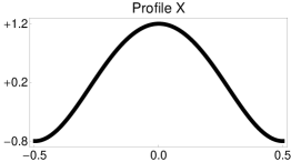
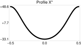
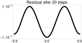
Figure 1: Profile $X$ with second derivative and residual for the data from (17).

In a simple discrete analog to Scheme 17 each profile function $X_{i}$ is identified with a vector $(X_{i}^{j})_{j=1..N}$ via $X^{j}_{i}={X_{i}{\left({-1/2+j/N}\right)}}$, where $k$ is supposed to be a multiple of $1/N$, and the derivative $X_{i}^{\prime}$ is approximated by centred finite differences. Moreover, integrals with respect to ${\varphi}$ are replaced by their Riemann sums and $x_{i}$ is computed by a discrete gradient flow for the function $x\mapsto\sum_{j=1..N}\Psi(x+X_{i}^{j})$. This numerical approach is illustrated in Figure 1 for the data

$${\gamma}=10,\qquad k=0.1,\qquad\Psi^{\prime\prime}{\left({x}\right)}=\exp{\left({-x}\right)},$$ (17)

with $N=800$ and $X_{0}{\left({{\varphi}}\right)}=\sqrt{{\gamma}}\pi^{-1}\cos{\left({2\pi{\varphi}}\right)}$. Under the iteration the functions $X_{i}$ converge to a wave train, that means a fixed point of $\mathcal{T}_{\gamma}$, with unimodal and even second derivative. Moreover, numerical simulations indicate that the limit profile is independent of the initial profile $X_{0}\in\mathcal{C}$.

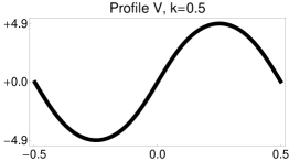
Figure 2: Profiles $X$ and $V$ for the data from (18).

Further numerical results are shown in Figure 2 and correspond to

$${\gamma}=50.,\qquad{k}\in\{0.1,\,0.3,\,0.5\},\qquad\Psi^{\prime\prime}{\left({x}\right)}=1+x^{2},$$ (18)

where $N$ and $X_{0}$ are chosen as above. Here we plot additionally the profile function $V=-{\omega}{X^{\prime}}$, which describes the atomic velocities in a wave train via $\dot{y_{j}}{\left({t}\right)}={V}{\left({kj-{\omega}{t}}\right)}$, compare (2).

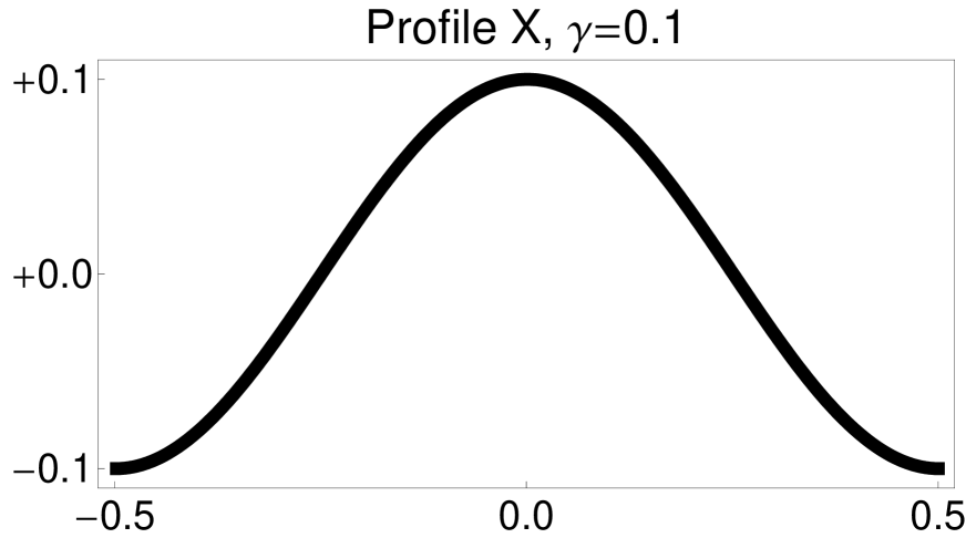
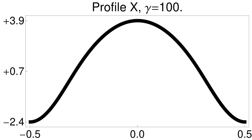
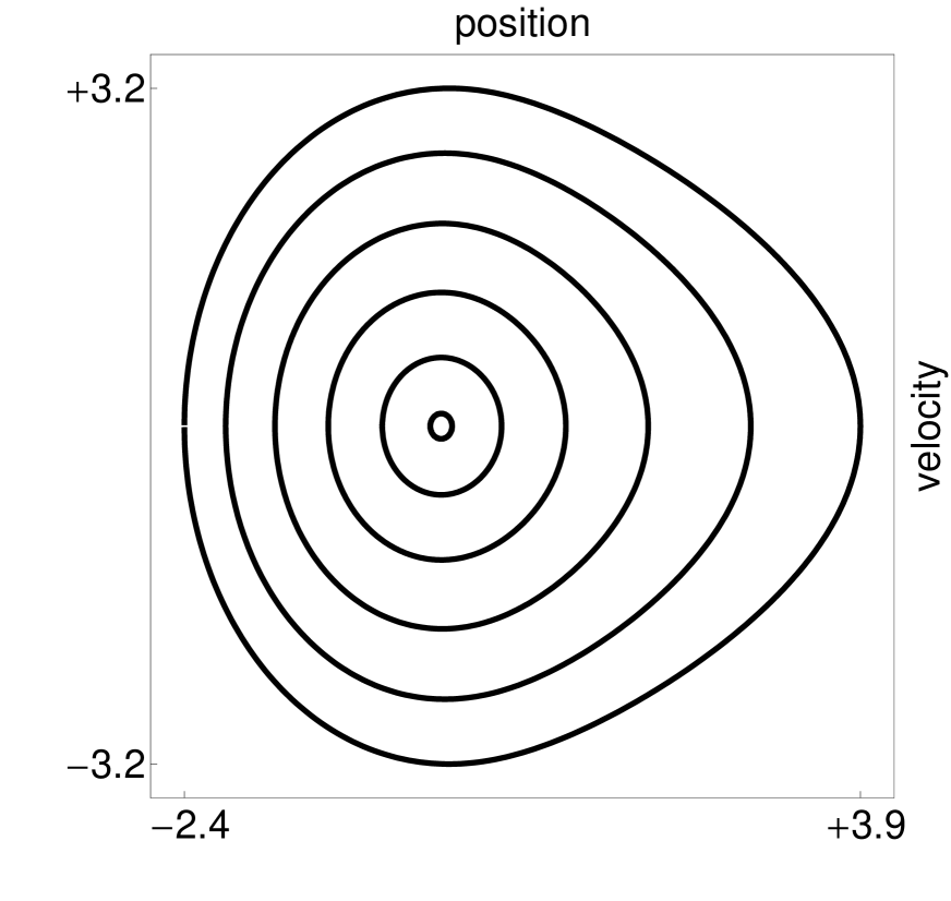
Figure 3: Simulations for the data from (19): Profiles $X$ and $V$ for minimal and maximal value of ${\gamma}$, and superposition of six traces of wave trains.

The simulations in Figure 3 correspond to

$${\gamma}\in\{0.1,\,3,\,12,\,30,\,60,\,100\},\qquad k=0.1,\qquad\Psi^{\prime\prime}{\left({x}\right)}=\exp{\big{(}-\max{\{x,\,0\}}^{2}\big{)}},$$ (19)

and illustrate how the wave trains depend on ${\gamma}$. The right picture shows the traces of the wave trains, that means the closed curves

$${\varphi}\mapsto{\big{(}{X{\left({{\varphi}}\right)}},\,{V{\left({{\varphi}}\right)}}\big{)}},$$

whose diameters increase with ${\gamma}$. Surprisingly, we find a nested family of curves: The traces for different values of ${\gamma}$ do not intersect, but all traces for $\tilde{{\gamma}}\leq{\gamma}$ fill out the interior of the trace for ${\gamma}$. This observation indicates the existence of a ‘hidden structure’ for the nonlinear advance-delay differential equation (8). In particular, there must be an equivalent planar Hamiltonian system such that the traces coincide with the level sets of the Hamiltonian. We cannot prove that the wave trains for fixed $k$ and increasing ${\gamma}$ give rise to a nested family of closed curves but mention that a similar phenomenon can be observed for wave trains in FPU chains, see [Her08, HR08].

References

• [BK04] O. M. Braun and Y. S. Kivshar, The Frenkel-Kontorova model: Concepts, Methods, and Applications, Theoretical and Mathematical Physics, Springer, 2004.
• [BZ06] P. W. Bates and Ch. Zhang, Traveling pulses for the Klein-Gordon equation on a lattice or continuum with long-range interaction, Discr. Cont. Dynam. Systems Ser. A 16 (2006), no. 1, 235–252.
• [DEFW93] D. B. Duncan, J. C. Eilbeck, H. Feddersen, and J. A. D. Wattis, Solitons on lattices, Physica D 68 (1993), 1–11.
• [DPB93] Th. Dauxois, M. Peyrard, and A. R. Bishop, Dynamics and thermodynamics of a nonlinear model for DNA denaturation, Phys. Rev. E 47 (1993), no. 1, 684–695.
• [Her08] M. Herrmann, Unimodal wave trains and solitons in convex FPU chains, arXiv:0901.3736, 2008.
• [HR08] M. Herrmann and J. Rademacher, Heteroclinic travelling waves in convex FPU-type chains, arXiv:0812.1712, 2008.
• [IJ05] G. Iooss and G. James, Localized waves in nonlinear oscillator chains, Chaos 15 (2005), no. 1, 015113:1–15.
• [IK00] G. Iooss and K. Kirchgässner, Travelling waves in a chain of coupled nonlinear oscillators, Comm. Math. Phys. 211 (2000), no. 2, 439–464.
• [IP06] G. Iooss and D. E. Pelinovsky, Normal form for travelling kinks in discrete Klein Gordon lattices, Physica D 616 (2006), no. 2, 327–345.
• [Kat05] Guy Katriel, Existence of travelling waves in discrete Sine-Gordon rings, SIAM J. Math. Anal. 36 (2005), no. 5, 1434–1443.
• [KZ08a] C. F. Kreiner and J. Zimmer, Heteroclinic travelling waves for the lattice Sine-Gordon equation with linear pair interaction, BICS preprint 1/08, 2008.
• [KZ08b]  , Travelling wave solutions for the discrete Sine-Gordon equation with nonlinear pair interaction, BICS preprint 3/08, 2008.
• [MJKA02] A. M. Morgante, M. Johansson, G. Kopidakis, and S. Aubry, Standing wave instabilities in a chain of nonlinear coupled oscillators, Phys. D 162 (2002), no. 1/2, 53–94.
• [Pan05] A. Pankov, Traveling waves and periodic oscillations in Fermi-Pasta-Ulam lattices, Imperial College Press, London, 2005.