Optimal Control at the Quantum Speed Limit
Abstract
Optimal control theory is a promising candidate for a drastic improvement of the performance of quantum information tasks. We explore its ultimate limit in paradigmatic cases, and demonstrate that it coincides with the maximum speed limit allowed by quantum evolution.
pacs:
Engineering a suitable Hamiltonian that evolves a given quantum system into a selected target state has acquired special relevance after the recent advent of quantum information science Nielsen and Chuang (2000). Here, the challenge is to perform quantum tasks (e.g. apply a quantum gate) in an accurate way while fulfilling the stringent requirements of fault tolerance. In this context quantum Optimal Control (OC) is considered a very promising tool, and different algorithms have been designed with this aim Krotov (1996); Khaneja et al. (2005). One of them exploits the Krotov algorithm Krotov (1996), a numerical recursive method which seeks the OC pulses necessary to implement the required transformation by solving a Lagrange multiplier problem Peirce et al. (1988). This technique has already been applied with success to a wide range of quantum systems Somloi et al. (1993); Peirce et al. (1988). One issue that is not yet fully understood however is what its limits are, and how these limits may be approached. In this work we will show that the effectiveness of the Krotov algorithm for quantum OC is related to fundamental bounds that affect the maximum speed at which a quantum system can evolve in its Hilbert space. Besides being of interest from a theoretical perspective, the discovery of such a constraint is also important for practical implementations.
For time-dependent Hamiltonians, bounds that relate the transition probabilities of a quantum system to its mean energy spread were set by Pfeifer Pfeifer (1993) and Bhattacharyya Bhattacharyya (1983), more than fifteen years ago. For time-independent Hamiltonians, these results have been extended to include dynamical constraints that involve also the energy expectation value of the evolving system Margolus and Levitin (1998). Moreover in a specific case Khaneja et al. evaluated the minimum time required to implement a given quantum transformation Khaneja et al. (2005). In the light of these results our aim is to explore the very limit of OC. In particular, we are interested to see whether the Krotov algorithm Krotov (1996) allows one to attain the ultimate bound set by quantum mechanics (for which we borrow from Margolus and Levitin (1998) the term Quantum Speed Limit (QSL)).
Several attempts to reconcile accuracy and speed in quantum control have been proposed so far (see Carlini et al. (2006); Gruebele and Wolynes (2007) and references therein). In particular, Carlini et al. Carlini et al. (2006) cast the time-OC problem into the commonly termed quantum brachistochrone problem: exploiting the variational principle they produce a collection of coupled non-linear equations whose solution (when it exists) yields the required optimal time-dependent Hamiltonian that minimizes the time evolution while satisfying certain constraints on the available resources. Our approach differs from that of Ref. Carlini et al. (2006) since we do not treat the duration of the process as a variable that enters in the optimization process. Instead, we set it to some fixed value and use standard quantum control optimization techniques to find the -long pulses which guarantee higher accuracy. The connection between OC and the QSL emerges at the time duration for which OC fails to converge.
Specifically, given an input state and a Hamiltonian that depends on the set of time-dependent control functions , we shall employ the Krotov algorithm Krotov (1996) to determine the optimal that minimizes the infidelity , which measures the distance between the target state and the time- evolved state under . The are constructed iteratively, starting from some initial guess functions . We then analyze the performance of the process as a function of and show that the method is able to produce infidelities arbitrarily close to zero only above a certain threshold , which we compare with the dynamical bounds that affect the system. We found a good agreement between these (in principle) independent quantities, meaning that the effectiveness of our control pulses is only limited by the dynamical bounds of the system. Considering the limited set of controls we allow in the problem, and the fact that our initial equations are not meant to optimize , this is a rather remarkable fact that suggests that OC is a possible candidate for an operational characterization of the QSLs of complex systems.
Even though our findings have been obtained in several different contexts, including for instance ordered Ising and Lipkin-Meshkov-Glick models, for the sake of clarity and for demonstration of the generality of the argument, in this Letter we shall focus on two paradigmatic examples: the Landau-Zener (LZ) model Zener (1932), and the transfer of information along a chain of coupled spins with Heisenberg interactions. The former case constitutes a basic step for the control of complex many-body systems, whose evolution, for finite size systems, is in many cases a cascade of LZ transitions Santoro et al. (2002). Adiabatic quantum computation Farhi et al. (2001) is known to be limited by avoided crossings in the time-dependent system Hamiltonian and by our inability to avoid excitation of the system. The spin-chain case is instead related to one of the central requirements for the construction of circuit-model quantum computers: an infrastructure that can rapidly and accurately transport qubit states between sites Bose (2007).
Landau-Zener model - The first example we consider is the paradigmatic case of the passage through an avoided level crossing
| (3) |
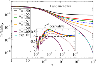
in which is the control function that we shall optimize through the Krotov algorithm. We start the evolution by preparing the system in the instantaneous ground state of and we assume as our target the ground state of , with (). As an initial guess for the control we follow Ref. Roland and Cerf (2002). Here on the basis of the adiabatic theorem Messiah (1962) the control pulse was selected through a differential equation , where is the instantaneous energy gap of the Hamiltonian (3), while . Starting from the defined above, we run the OC algorithm for various values of the total time . The results are reported in Fig. 1 by plotting the infidelity as a function of the iterations of the algorithm. When , the infidelity does not converge to zero, being its curvature asymptotically flat. On the contrary, by progressively increasing towards and above , the curvature changes sign and the infidelity in the large iteration limit decreases exponentially, as confirmed by the fit in Fig. 1. In the inset of Fig. 1, data for the second derivative of the infidelity logarithm with respect to the logarithm of for different are shown: the derivative starts to cross the zero line for , and for it clearly becomes negative. These findings are reflected by the study of the pulse shape of the optimization process (data not shown). For , the pulse develops a peak which grows indefinitely by increasing and the control seems unable to converge towards an optimal shape. On the contrary, when , after a certain number of iterations, the shape becomes stable, and only small corrections of the order of the infidelity take place. Remarkably, the peculiar feature of the initial guess of being almost constantly zero for most of the central part of the evolution is preserved by the recursive optimization of OC Krotov (1996), suggesting that for this simple model an estimation of a finite resource QSL bound for can be deduced by a time-independent formula, assuming as the Hamiltonian. In other words, for most of the evolution time the dynamics can be effectively described by a time-independent Hamiltonian, which we can use to analytically estimate the QSL. This can be quantified with the Bhattacharyya bound Bhattacharyya (1983), yielding
| (4) |
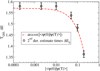
where is the energy variance of calculated on the initial state , i.e. . This approach has the advantage of providing a bound for that is independent of the effective shape of the selected pulse. Finally, in Fig. 2 we show a comparison between the estimate through the second derivative of the infidelity and the theoretical time-independent estimate (4) for various ratios. We stress that here we have no fitting parameters. The excellent agreement shows that the OC efficiency is ultimately set by the dynamical bound of Eq. (4).
Quantum state transfer - We now apply our analysis to a scheme for information transfer in a spin chain Bose (2007). In this context a notion of QSL for spin chains was introduced in Ref.Yung (2006) where the velocity of the information propagation was optimized with respect to the constant interactions among spins in the chain. This is of course quite different from the approach we introduce here where the couplings are given and the information transfer is sped up by using properly tailored external pulses. The model consists of a one-dimensional Heisenberg spin chain of length described by the Hamiltonian , where are the Pauli spin matrices, is the coupling strength between nearest-neighbour spins, is the relative strength of an external parabolic magnetic potential, and represents the position of the external potential minimum at time (in units of ) along the axis of propagation Balachandran and Gong (2008). Due to the conservation of the component of the magnetization, we can restrict our analysis to the sector with a single spin-up only, so that a general state is described by , where represents the state where the -th site has its spin pointing up, and all other sites have spins pointing down. The states form a complete orthonormal basis for our Hilbert subspace. Our goal is to evolve the initial state to the final state , i.e. to transport a spin up state from the first site to the final site of the chain. In Ref. Balachandran and Gong (2008) this was achieved by invoking the adiabatic approximation, which relies on the fact that slowly moving the parabolic magnetic potential along the chain allows the spin-up to migrate from the leftmost site to adjacent sites via a nearest-neighbour swapping, while interactions between sites far from the field minimum are frozen. Specifically, the transfer was obtained by assuming pulses of the form and , and by working in a regime of large (ideally infinite) transmission time . In our approach, we shall use instead the Krotov method to find the OC functions and using pulses similar to those of Ref. Balachandran and Gong (2008) as an initial guess: this allows us to shorten the transfer time beyond what is allowed by the adiabatic regime. Once again, we optimize the controls for different values of in an effort to identify the minimum transfer time allowed by the selected controlling Hamiltonian. For each selected the optimization algorithm stops either after a certain number of iterations (of the order of ) or when the infidelity reaches a certain fixed target threshold .
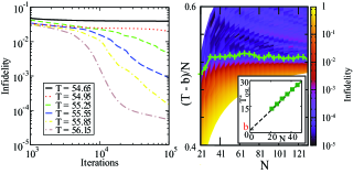
The results obtained are shown in Fig. 3 and resemble those we have seen in the LZ model. In particular, as shown in Fig. 3 (left) the infidelity appears to converge to zero only for values of that are above a certain critical time . On the contrary, for the convergence of the infidelity slows down, providing numerical evidence of a non-zero asymptote for . In contrast with the LZ case however, the dependence of with the iteration number is now less regular, reflecting the fact that the spin-chain dynamics is more complex than for the LZ model. Consequently, for the present model the sign of the second derivative cannot be used as a reliable signature of . Nonetheless, a numerical estimate for such quantity can been obtained by considering the smallest time which allows us to achieve the target infidelity threshold in a fixed number of algorithm iterations (the result does not depend significantly on the value of and ). Apart from the case of small , where boundary effects are more pronounced, the resulting appears to have a linear dependence on the chain length – see Fig. 3 (right).
For a comparison with an independent theoretical estimate of , we cannot directly use the Bhattacharyya bound (4), since in this case we are not allowed to treat the Hamiltonian as approximately time-independent. Nevertheless, a bound on the minimal transferring time can be obtained by considering the mean energy spread, obtained by averaging the instantaneous energy spread of the system of the time-dependent Hamiltonian over the time evolution . We define this by , where is the energy spread and is computed on the state , and labels different choices of . For , we follow Ref. Pfeifer (1993) and take to be either the initial state or the target state , whichever results in the smaller . For , we choose , which means we effectively divide the total evolution time into smaller intervals over which can be assumed to be constant, and apply to each of them the Bhattacharyya bound Bhattacharyya (1983) for time-independent Hamiltonians. The bound on the minimum transfer time is then given by , which needs to be satisfied by any that brings to the target state in a time . Since we have taken the time average of the bound, we interpret the quantum speed limit as describing the minimum transfer time ‘per-site’. In Fig. 4 (left), we report as a function of time for two different total transfer times. The energy spread is almost constant save near the final time, where large oscillations are present, corresponding to the deceleration of the spin-wave. The picture that arises is that OC finds a solution that initially accelerates the spin excitation, and then transfers it with constant velocity up to the end of the chain, where deceleration occurs. The average energy spreading is larger for smaller time transfer allowing for a higher average excitation velocity. We finally compare the estimated optimal time from Fig. 3 (right) with the analytical estimate of the QSL given above. The results are reported in Fig.4 (right) where the two quantities are compared: both estimators are linearly dependent on , but the numerical results show an improvement over the theoretical prediction by a factor of , which we attribute to the difficulty in formulating the quantum speed limit for our many-body problem. One can think of the optimal transfer of the excitation as being facilitated by a cascade of effective swaps.
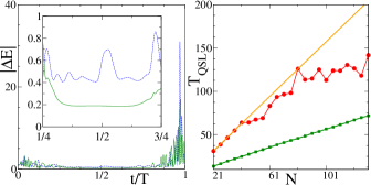
As before, the agreement of scaling of the two results shows that even in the presence of additional constraints the OC reaches the ultimate dynamical bounds set by quantum mechanics. Indeed, we achieved an improvement of the transfer time with respect to Ref. Balachandran and Gong (2008) of up to two orders of magnitude. It is also worth mentioning that we achieved a transfer time faster than that obtained (for Ising coupling) in Ref. Khaneja and Glaser (2002). Interestingly enough, however, our method only uses single-site local pulses while in Ref. Khaneja and Glaser (2002) this was achieved using global pulses that operate jointly on the whole chain.
In summary, we have demonstrated that there are fundamental constraints governing the efficiency of Krotov quantum OC algorithm dictated by the maximum speed at which a quantum state can evolve in time. These results provide a further link between control theory and quantum dynamics.
We thank A. Carlini for discussions, and the bwGRiD (http://www.bw-grid.de) for the computational resources. We acknowledge financial support by SFB/TRR21, and the EU under the contracts MRTN-CT-2006-035369 (EMALI), IP-EUROSQIP, and IP-SCALA.
References
- Nielsen and Chuang (2000) M. Nielsen and I. L. Chuang, Quantum Computation and Quantum Information (Cambridge University Press, 2000).
- Krotov (1996) V. F. Krotov, Global Methods in Optimal Control Theory (Marcel Dekker, New York, 1996).
- Khaneja et al. (2005) N. Khaneja et al., J. Mag. Res. 172, 296 (2005).
- Peirce et al. (1988) A. P. Peirce, M. A. Dahleh, and H. Rabitz, Phys. Rev. A 37, 4950 (1988); I. R. Sola, J. Santamaria, and D. J. Tannor, J. Phys. Chem. A 102, 4301 (1998); T. Calarco et al., Phys. Rev. A 70, 012306 (2004).
- Somloi et al. (1993) J. Somloi, V. A. Kazakov, and D. J. Tannor, Chemical Physics 172, 85 (1993); S. Montangero, T. Calarco, and R. Fazio, Phys. Rev. Lett. 99, 170501 (2007).
- Pfeifer (1993) P. Pfeifer, Phys. Rev. Lett. 70, 3365 (1993).
- Bhattacharyya (1983) K. Bhattacharyya, J. Phys. A: Math. Gen. 16, 2993 (1983).
- Margolus and Levitin (1998) N. Margolus and L. B. Levitin, Physica D 120, 188 (1998); V. Giovannetti, S. Lloyd, and L. Maccone, Phys. Rev. A 67, 052109 (2003); L. B. Levitin and T. Toffoli, arXiv:0905.3417, (2009).
- Carlini et al. (2006) A. Carlini et al., Phys. Rev. Lett. 96, 060503 (2006).
- Gruebele and Wolynes (2007) G. Gruebele and P. G. Wolynes, Phys. Rev. Lett. 99, 060201 (2007).
- Zener (1932) C. Zener, Proc. Royal Soc. A 137, 696 (1932).
- Santoro et al. (2002) G. E. Santoro et al., Science 295, 2427 (2002).
- Farhi et al. (2001) E. Farhi et al., Science 292, 472 (2001).
- Bose (2007) S. Bose, Contemporary Physics 48, 13 (2007).
- Roland and Cerf (2002) J. Roland and N. J. Cerf, Phys. Rev. A 65, 042308 (2002).
- Messiah (1962) A. Messiah, Quantum mechanics, vol. 2 (North-Holland, Amsterdam, 1962).
- Yung (2006) M.-H. Yung, Phys. Rev. A 74, 030303 (2006).
- Balachandran and Gong (2008) V. Balachandran and J. Gong, Phys. Rev. A 77, 012303 (2008).
- Khaneja and Glaser (2002) N. Khaneja and S. J. Glaser, Phys. Rev. A 66, 060301(R) (2002).