Quiet Planting in the Locked Constraint Satisfaction Problems
Abstract
We study the planted ensemble of locked constraint satisfaction problems. We describe the connection between the random and planted ensembles. The use of the cavity method is combined with arguments from reconstruction on trees and the first and the second moment considerations. Our main result is the location of the hard region in the planted ensemble. In a part of that hard region instances have with high probability a single satisfying assignment.
keywords:
Constraint Satisfaction Problems, Planted Random Ensemble, Belief Propagation, Reconstruction on Trees, Instances with a Unique Satisfying Assignment.AMS:
90C27 68Q25 05C80Constraint Satisfaction Problems (CSPs) are very general in their nature: Consider a set of discrete variables and a set of Boolean constraints; the problem consists in finding a configuration of variables that satisfies all the constraints or in proving that no such configuration exists. As such, CSPs are a subject of interest in many different fields such as computer science, discrete mathematics, physics, engineering and computational biology. Random ensembles of CSPs are a fertile source of research activity; as hard benchmarks they serve for testing new algorithmic ideas [5, 31], they are used to create efficient coding schemes [14, 15], to model complex glass forming liquids [4, 23], or to understand the origin of average computational hardness [30, 43]. Combining know-how from many branches of mathematics, computer science and statistical physics seems to be a fruitful strategy for the understanding of these stunning objects and of their very rich behavior.
The most commonly studied random ensembles of CSPs are created by choosing the graph of variables and constraints as a random bipartite graph with a certain left and right degree distribution. Another natural way of creating a random instance, called planting, is to first assign a configuration to all variables, and then to choose only constraints compatible with this configuration. Both these ensembles can be useful to mimic instances created in some practical applications, as e.g. the low density parity check codes [14]. In particular planted instances may be created in adaptive situations when only constraints satisfied by the current state of variables can be added.
By planting, we create by definition a satisfiable instance. Such instances are particularly useful as benchmarks to evaluate the performance of incomplete solvers, such as stochastic local search [38]. Based on the example of the planted K-satisfiability problem it is, however, often anticipated that the planted ensemble is algorithmically easier than the random one because a bias towards the planted assignment is created in the graph. Also, for most of the studied problems, it was proven that at large density of constraints is it indeed easy to find a satisfying assignment near to the planted one, see e.g. [3, 7, 13]. On the other hand if the planted ensemble would be algorithmically hard in some region of parameters than these instances could serve as one-way functions and have applications in cryptography. Yet, compared to the random ensemble, relatively little is known about the existence, size and properties of algorithmically hard regions in the planted ensemble.
In this paper we study a way of planting an assignment which changes only in a minimal way the properties of the random ensemble. We call this a quiet planting. Although the concept of quiet planting was introduced in [24], many result were actually first demonstrated and used as a tool for proofs in [2]. Both these works, however, were mainly concentrated on the coloring problem (and on hyper-graph bi-coloring). In the present work we generalize this idea and we will focus on quiet planting in the so-called locked CSPs, introduced recently in [43, 42]. On one hand, the locked CSPs have a very interesting phase diagram which description-wise is much simpler than the one of the graph coloring or K-satisfiability. On the other hand they are much harder algorithmically and the boundaries between the easy and hard regions are, unlike in the coloring or K-satisfiability, relatively well understood (at least on the heuristic level of the cavity method [43, 42]). This special behavior stems from the fact that in the locked problems the space of solutions consists of points separated by an extensive (i.e. ) Hamming distance instead of clusters of solutions.
Here, we combine the idea of quiet planting with the special behavior of the locked CSPs and obtain random CSPs ensembles with many interesting properties that are summarized in Sec. 1 in the context of related works. In Sec. 2 we introduce the necessary definitions and notations, and in Sec. 3 we summarize the phase diagram of the locked problems derived in [43, 42]. In Sec. 4 we argue about the equivalence between the random and the planted ensemble based on heuristic considerations and on a second moment computation. In Sec. 5 we describe the interesting phase where instances of our problems have with large probability a single solution. Finally, in Sec. 6 we discuss the algorithmic hardness of the planted instances, and compute the critical degree beyond which instances become easy to solve. We conclude the paper with a list of open problems in Sec. 7.
1 Main results and related works
The results of this paper apply to the factorized locked CSPs, see Defs. 2, 4. We list in six points the most important contributions of the present article:
-
(i)
The planted configuration is equivalent to randomly sampled satisfying assignment: The idea of quiet planting is to plant a configuration that in many important properties does not differ from a satisfying assignment sampled uniformly at random on the resulting graph. Such a problem is closely related to the reconstruction on trees [10, 34, 26] where we consider an assignment taken uniformly at random from all the satisfying ones. Constructing such an assignment on a tree is always possible in polynomial time, as the exact marginal probabilities can be obtained via the belief propagation (BP) algorithm. On random graphs, uniform sampling is in general exponentially costly. However, the quiet planting can be achieved asymptotically on the factorized CSPs, see Def. 4. In a statistical physics language quiet planting is possible whenever the quenched entropy equals the annealed one, see condition (18). The possibility of quiet planting and its relation to a concentration property (18) was previously discussed for other constraint satisfaction problems in [32, 2, 24].
-
(ii)
Equivalence between the planted and the random ensemble in the satisfiable phase: Many properties of the planted ensemble created via quiet planting can be deduced from the properties of the purely random ensemble. Among others, in the satisfiable phase the random and planted ensembles are asymptotically equivalent, see Def. 8. Such equivalence can also be established rigorously based on a second moment argument, as in [2]. In the factorized locked problems treated in this article the second moment is able to pin the satisfiability threshold sharply and hence the equivalence between the planted and the random ensemble holds in the whole satisfiable phase.
-
(iii)
Equivalence between planted and satisfiable ensembles: Based on heuristic (cavity) arguments we conjecture that the planted ensemble is in the factorized locked problems asymptotically equivalent to the ensemble of satisfiable instances in the whole range of constraint densities. In particular, this means that one can recognize easily almost all the rare satisfiable instances above the robust reconstruction threshold by using belief propagation. We stress here that we do not expect this equivalence to be true in the non-locked CSPs, such as graph coloring or K-satisfiability.
-
(iv)
Easy-hard-easy transition: Next to the interesting conceptual results, the most important practical result is the identification and the location of the region where the instances from the planted ensemble of the factorized locked problems are on average computationally hard. We show that an easy-hard-easy pattern for finding a solution appears in the planted ensemble as the constraint density is increased, where easy means that an on-average polynomial algorithm is known, while hard means that no on-average polynomial algorithm is known (and maybe does not exist). We conjecture that the two boundaries of the hard phase correspond to two different reconstruction thresholds – the onset of hardness coincides with the small noise reconstruction threshold [42], called the dynamical transition in the physics literature [22], and the end of the hard region is given by the threshold for the robust reconstruction [16]. This last point also corresponds to the Kesten-Stigum bound for the canonical reconstruction on trees [19, 20], and to the spin glass local instability in the purely random ensemble [29]. We also show that outside the hard region algorithms based on belief propagation are able to find solutions efficiently. In particular in the high average degree easy region, the belief propagation algorithm converges directly to the planted solution.
-
(v)
Hard satisfiable benchmarks: Given we have located the values of parameters where the instances of the planted ensemble are hard, these can serve as very challenging satisfiable benchmarks. Such benchmarks are in particular interesting for the evaluation of regions in which incomplete solvers work —or do not work— in polynomial (linear) time. Note that for complete exhaustive solvers the locked problems are not necessarily harder than the canonical K-satisfiability. On the contrary, locked constraints produce more implications when a variable is fixed, hence exhaustive branch-and-bound techniques might come to a decision relatively faster than in the random K-satisfiability.
-
(vi)
Instances with unique satisfying assignment (USA): We show that beyond the threshold corresponding to the satisfiability threshold in the random ensemble the planted instances have with high probability a single satisfying assignment (or a pair of them in case a global symmetry is present). Moreover depending on the constraint density these USA instances can be found in the hard or in the easy region. Some USA instances are extensively used in evaluation of quantum algorithms, see e.g. [40, 12]. In these previous works these instances are, however, generated with exponential cost, and their classical typical computational hardness has not been evaluated.
A large part of our results is based on the heuristic cavity method approach [28]. We were also able to prove part of our results for the -in- SAT problem on random regular graphs using computations of the second moment and the expander property. This includes some results about the equivalence between the planted and random ensembles in the satisfiable phase, and the uniqueness of the satisfying assignment in the unsatisfiable phase. Completing and extending these proofs to the other locked factorized CSPs should be possible although more involved.
| RANDOM | ||||
|---|---|---|---|---|
| BP, random init. | converges | converges | converges | does not |
| BP fixed point | uniform | uniform | uniform | |
| of solutions | exponential | exponential | none | none |
| finding solution | easy | hard | ||
| reconstruction | not possible | possible |
| PLANTED | ||||
|---|---|---|---|---|
| BP, random init. | converges | converges | converges | converges |
| BP fixed point | uniform | uniform | uniform | planted |
| BP, planted init. | converges | converges | converges | converges |
| BP fixed point | uniform | planted | planted | planted |
| of solutions | exponential | exponential | one/two | one/two |
| finding solution | easy | hard | hard | easy |
| reconstruction | not possible | possible | possible | possible |
| robust recons. | not possible | not possible | not possible | possible |
2 Definitions and notations
In this section we specify the class of constraint satisfaction problems to which our results apply. The crucial notions will be the definition of a locked [43] and factorized constraint satisfaction problem. It is only on the factorized problems where there is a very close relation between the usual random and the planted ensemble, as discussed in [24]. It is also the fact that in the locked problems solutions (i.e. satisfying assignments) are mutually far from each other in terms of their Hamming distance [43] that makes them particularly interesting for considerations in this context.
Definition 1.
A constraint containing variables, the domain of each variable being , is a function from to . If the function evaluates to () we say that constraint is satisfied (not satisfied). A constraint is locked if and only if there are no two satisfying assignments of variables which would differ in a single value (out of the ones).
In this paper we will consider for concreteness binary variables, that is , but the results are generalizable to larger domain sizes.
Definition 2.
A constraint satisfaction problem consists in deciding if there exists a configuration of variables which satisfies simultaneously a set of constraints. A constraint satisfaction problem is called locked if and only if all the constraint are locked and each of the variables belongs to at least two different constraints.
Thus anytime we speak about a locked problem we implicitly suppose that the corresponding factor-graph does not have any leaves (variables of degree one). The degree of a variable is defined as the number of constraints to which the variable belongs, while the degree of a constraint is the number of variables it contains.
We shall illustrate our findings on the so called occupation constraint satisfaction problems [33, 42].
Definition 3.
In occupation problems every constraint depends only on the sum of the variables it contains. Thus every occupation constraint containing variables can be characterized by a binary component vector such that the constraint is satisfied if and only if the sum of the variables is such that .
An occupation constraint is locked if and only if for all we have . We will consider occupation problems where every constraint contains variables and is given by the same vector . To give an example of this notation, the vector corresponds to the -in- SAT problem (also called exact cover), which is indeed locked. The vector corresponds to the hyper-graph bi-coloring problem, which is not locked (since there are two neighboring s). Many other examples can be found in [42]. For problems which do not have other name established in the literature, we will use the notation i-or-j-…-in-K SAT for a vector with non-zero components ,, etc.
Let us now write the belief propagation (BP) equations [35, 25, 27] for the occupation constraint satisfaction problems. The basic quantities in BP are messages. We define as the probability (over all satisfying assignments) that the variable has value given that belong only to constraint . The BP equations approximate these probabilities by messages by assuming that the factor graph [25] underlying the CSP is a tree
| (1) |
where is a normalization constant assuring , is the set of neighbors of , are neighbors of except , and the sum over is over all values variables can take. Fig. 1 shows the corresponding part of the factor graph.

We define to be the probability (over all satisfying assignments) that a variable is occupied. The BP estimate of the probability that a variables is occupied is
| (2) |
Note that if an assignment is a solution of the locked problem, then , is a fixed point of the BP equations (1). If the underlying factor-graph is a tree then the fixed point of the BP equations is unique and and in the fixed point (note that on a tree the problem is not locked). On a graph with cycles this is not the case in general. We will call a BP fixed point asymptotically () exact on a random ensemble of graphs if and for almost all and with high probability, where is the number of nodes in the graph.
All our results are restricted to ensembles of constraint satisfaction problems where at least one BP fixed point is asymptotically exact. We define such ensembles in the remaining of this section. A graph ensemble is locally tree-like if the shortest loop going trough a random node has w.h.p. length diverging as . Families of sparse random graphs, i.e. the degree distribution of variables does not depend on , are locally tree-like as long as the mean of is finite. The variable degree distributions we will be using mostly are:
-
•
Regular .
-
•
Truncated Poisson , for . The average degree in this case is .
In order to generate random graphs with a given variable degree distribution, one can apply the following algorithm:
-
•
Repeat until : Draw random numbers from distribution .
-
•
Consider legs going from every constraint, order them arbitrarily and index them from to , consider legs from every variable , order them arbitrarily and index them from to .
-
•
Repeat until there are no double edges: Draw a random permutation of numbers and connect -th leg from constraints with -th leg from variables.
We define an iteration of the belief propagation algorithm as taking all the KM edges in a random order and updating the message according to eq. (1).
Definition 4.
A given instance of a constraint satisfaction problem is factorized if and only if the belief propagation equations initialized randomly converge almost surely (with probability approaching one as the number of variables ) to a uniform fixed point, i.e., the value of is the same for almost all edges .
Note that it is a non-trivial task to provably decide if a problem satisfies this definition, and the answer depends on the degree distribution. In practice we generate a large random instance of the problem, initialize BP randomly and iterate. We observe that the result (i.e. if the condition in def. 4 is satisfied or not) is the same on almost all large random instances. The condition of def. 4 can hence be checked computationally with a small computer-time effort.
Definition 5.
Let be the number of satisfying assignments of an instance of the constraint satisfaction problem . We define the annealed entropy to be
| (3) |
where the expectation is over the graph ensemble. The quenched entropy is defined as
| (4) |
Definition 6.
The following statement stands on the basis of the cavity method: If a BP fixed point is asymptotically exact (for a given random graph ensemble) then the Bethe entropy (5) is equal to the quenched entropy (4).
The following result was obtained in [33] (section 5.1.2) for the occupation constraint satisfaction problems, and we conjecture it is general: The annealed entropy (3) is equal to the Bethe entropy evaluated in the uniform BP fixed point (when more than one uniform BP fixed point exists then consider the maximum of the Bethe entropy over the uniform fixed points).
If the problem is factorized and the uniform BP fixed point is asymptotically exact then the annealed entropy is equal to the quenched entropy, . Our results in the remaining of this paper apply to random constraint satisfaction problems where indeed (at least in some region of constraint densities). This condition is sometimes amenable to a rigorous proof, as it is in general weaker than , see [2]. If we are, however, interested in a fast heuristic check, then checking if the random constraint satisfaction problem is factorized may be more suitable.
3 Basic properties of the random factorized locked problems
For the locked problems, a detailed empirical analysis was done in [43, 42]. In this section we summarize the most relevant results (heuristically reasoned conjectures) of those works. It was found that a locked CSP is factorized in (at least) the two following cases:
-
(a)
Any locked problem on random regular graphs, that is when every variable is contained in constraints. On regular graphs, the uniform fixed point of the BP equations then satisfies
(7) (8) where is the normalization. For the probability that a variable in occupied one has in this case in the limit
(9) Let us call the probability that a constraint contains occupied variables. Then
(10) -
(b)
The balanced locked problems [42], are problems where the vector is symmetric, for all and this 0-1 symmetry is not spontaneously broken (that is when a satisfying assignment chosen uniformly at random has the same number of ’s and ’s up to a factor). Note that the absence of the symmetry breaking might depend on the degree distribution . In the balanced locked problems the uniform BP fixed point . For the probability that a constraint contains occupied variables we have here
(11)
A particularly simple case of (a) is the -in- SAT where . If every variable has connections and every constraint has to contain exactly occupied variables, then the number of occupied variables is exactly , and thus .
The authors of [43, 42] conjectured that when the limit of the Bethe entropy for a locked problem is positive, then the Bethe entropy is equal to the quenched entropy, and the BP fixed point reached from random initialization is asymptotically exact. If the Bethe entropy is negative then no satisfying assignment exists with high probability.
The Bethe entropy for all the balanced locked problems reads
| (12) |
where is the average degree of a variable (as we speak only about locked problems, the degree distribution has to have a zero weight on variables of degree zero and one). For all the locked problems on random regular (degree fixed to ) graphs the entropy reads
| (13) |
where , is the fixed point of eqs. (7-8). This entropy simplifies further for the -in- SAT on regular graphs (where the values of the s obey the simple form discussed previously) where we get an explicit formula
| (14) |
where is the entropy function.
The satisfiability transition is then defined by
| (15) |
for the corresponding entropy function. For the problem has almost surely exponentially many solutions (the exponent being given by ) whereas for the problem almost surely does not have any solution.
The authors of [43, 42] also argued about the existence of a second phase transition in the locked problems, , traditionally called in the physics literature the dynamical transition because of its connection to dynamics of glasses [32]. This critical point separates a region where for being a typical satisfying assignment the , defines a stable fixed point of the BP equations (1), from a region where this does not hold anymore. In other words, if an infinitesimal perturbation is introduced to these messages, the iteration of (1) goes back to the solution-related fixed point for , but not for . The authors of [43, 42] also conjectured that for a typical solution does not have solutions up to an extensive (i.e. ) Hamming distance, whereas for there are other solutions at sub-extensive (i.e. ) Hamming distance. Let us call the phase corresponding to the separated phase, and the one corresponding to the non-separated phase.
For the locked problems on regular graphs, the following inequality always holds: . In other words at the system is in the non-separated phase while for the solutions are always separated and the solution-corresponding fixed points are stable. For the balanced locked problems whenever the degree of every variable is larger or equal to three the system is in the phase where solutions are separated. When the fraction of variables of degree two is positive, , then the expression for follows [42]:
| (16) |
There is a deep connection between this dynamical threshold and the reconstruction problem [10, 34, 26]. In the reconstruction problem one creates a tree with the same degree properties as the random graph. Then one considers a satisfying assignment chosen uniformly at random from all the possible ones. The reconstruction problem finally consists in deciding whether this assignment on the leaves of the tree contains some information about the value assigned to the root. In the locked problems the value of the root is always uniquely implied by the values of the leaves, as follows from the very definition of these problems. However, if an infinitesimal noise is introduced on the leaves then there is no information left if and only if . This value was called the small noise reconstruction threshold in [42].
To summarize, the random locked factorized problems are in the non-separated phase for , which was shown to be algorithmically easy in [43, 42]. For the space of solutions is separated and it is then hard to find any solution. For no solution exists anymore.
| A | ||||||||
| 00100 | 3 | 4* | 1.256 | 1.853 | 2.821 | 2.513 | 2.827 | 3.434 |
| 0001000 | 4 | 6* | 1.904 | 3.023 | 4.965 | 2.856 | 3.576 | 5.144 |
| 000010000 | 5 | 8* | 2.337 | 3.942 | 6.994 | 3.116 | 4.276 | 7.039 |
| 5-in-10 | 5 | 10* | 2.660 | 4.794 | 8.999 | 3.325 | 4.944 | 9.009 |
| 6-in-12 | 6 | 12* | 2.918 | 5.455 | 11.00 | 3.502 | 5.586 | 11.00 |
| 01010 | 4* | 1.904 | 3.594 | 2.856 | 4 | |||
| 0101010 | 6* | 2.660 | 5.903 | 3.325 | 6 | |||
| 010101010 | 8* | 3.132 | 7.978 | 3.654 | 8 | |||
| 0010100 | 6 | 46* | 2.561 | 5.349 | 45.00 | 3.260 | 5.489 | 45.00 |
| 000101000 | 7 | 29* | 2.975 | 6.650 | 28.00 | 3.542 | 6.708 | 28.00 |
| 001010100 | 8 | 3.110 | 7.797 | 3.638 | 7.822 | |||
| 010010010 | 6 | x | 2.173 | 4.896 | x | 3.014 | 5.083 | x |
| A | ||
|---|---|---|
| 0100 | 3 | 3* |
| 01000 | 3 | 4* |
| 010000 | 3 | 5* |
| 0100000 | 3 | 6* |
| 001000 | 4 | 5* |
| 0010000 | 4 | 6* |
| A | ||
|---|---|---|
| 010100 | 5 | |
| 0101000 | 6 | |
| 010010 | 4 | 10 |
| 0100100 | 4 | 14 |
| 0100010 | 4 | 7 |
4 Equivalence of the random and planted ensembles
The planted ensemble of graphs, which is the main subject of the present paper, is created in the following way:
-
(i)
Make each of the variables occupied with probability (9), call the number of occupied variables .
-
(ii)
Choose a degree sequence from the probability distribution in such a way that .
-
(iii)
For each constraint, and according to the probabilities (10), choose the number of occupied variables to which it is connected. Repeat until . Here are the indexes of the occupied variables. If this condition cannot be achieved go back to step (i) and repeat it until the condition is achievable.
-
(iv)
Now consider the legs going out of every constraint , order them arbitrarily and index them by going from to . Consider legs going out from every occupied variable and index them. Choose a random permutation of numbers, and connect the leg with index going out from occupied variables to the leg with index going out from constraints. Do the same with the empty variables and the remaining legs going out from the constraints. Repeat until there are no double edges.
Note that there are several other models how to plant a solution (e.g. choose exactly the integer value of occupied variables in the step (i)), we could have chosen any other which is equivalent (for typical properties) to the above one in the limit.
Definition 7.
Call a property of a large random graph drawn from a given random ensemble a thermodynamic property if and only if in the limit the probability that this property holds is smaller than , where is some constant.
In statistical physics of random systems it is often the case that large deviations are exponentially rare and hence all usually considered properties are thermodynamic in this sense. Without attempting a rigorous proof, in statistical physics the following examples are often assumed to be thermodynamic properties: The degree distribution, the entropy density, the fraction of occupied variables in a random satisfying assignment, the distance between two random satisfying assignments, etc. Properties that are not thermodynamic are all those relying on the behavior of exponentially rare instances, e.g. moments of some exponentially large quantities, as for instance the number of satisfying assignments.
Definition 8.
Consider two ensembles of random graphs and , we call the two ensembles asymptotically equivalent if and only if every property that is thermodynamic in ensemble is thermodynamic in ensemble , and vice versa.
Definition 9.
The planting is called quiet if the corresponding planted and random ensembles are asymptotically equivalent.
Quiet planting intuitively means that if one is given a large random graph, one is not able to tell if that graph was drawn from the random or from the planted ensemble. This is because properties that are usually measured to distinguish the two graphs ensembles are thermodynamic (even if proving they are thermodynamic might be in general difficult).
The close relation between the random and the planted ensemble was explored in [2] for the random graph coloring and bi-coloring problems, see Theorem 6 and Theorem 7 in the appendix A of [2]. In statistical physics the quiet planting for graph coloring was discussed in [24].
Proposition 10.
Denote the number of satisfying assignments of an instance drawn from the random ensemble. If is a thermodynamic property, i.e.
| (17) |
and if the annealed entropy is equal to the quenched one, i.e.
| (18) |
then the planted ensemble and the random ensemble are asymptotically equivalent.
of Prop. 10.
In the random ensemble we are drawing graphs uniformly from all the graphs with a given degree distribution. In the planted ensemble we are drawing from the same set of graphs but with probability proportional to . Since (17) and (18) hold by assumption for the random ensemble, relation (17) holds for some also for the planted ensemble. Indeed, if (17) holds and if there would be larger than exponentially small probability that planting draws instances with then (18) could not hold. For every other thermodynamic property, i.e. such that large deviations are exponentially rare, the the same argument applies. ∎
Statements equivalent to Prop. 10 first appeared in eq. (4) and Theorem 6 in [2]. Note that when the concentration condition (18) can be proven in a stronger form, then the condition on the exponentially rare large deviation can be weakened.
In statistical physics, using the cavity method arguments, the condition (18) can be evaluated. As we state at the end of sec. 2, when the Bethe entropy is asymptotically exact then the factorization and the equality of the quenched and annealed entropies are equivalent. Hence quiet planting is possible in all the factorized problems as long as the Bethe entropy is asymptotically exact. In the non-locked factorized problems, such as the random graph coloring, condition (18) ceases to be true strictly before the satisfiability threshold, as discussed in [24].
In the next section we argue that in the factorized locked problems (18) holds up to the satisfiability threshold, and hence the planted and the random ensembles are asymptotically equivalent for the factorized locked problems in the whole range of parameters corresponding to the satisfiable phase on the random ensemble.
4.1 Second moment argument
Relation (18) is in general rather hard to prove rigorously. Achlioptas and Coja-Oghlan [2] used instead a stronger condition which they proved for the coloring and the bi-coloring of factor-graphs problem for sufficiently sparse graphs.
For the factorized locked problems we conjecture that the relation holds in all the factorized locked problems on the purely random ensemble as long as .
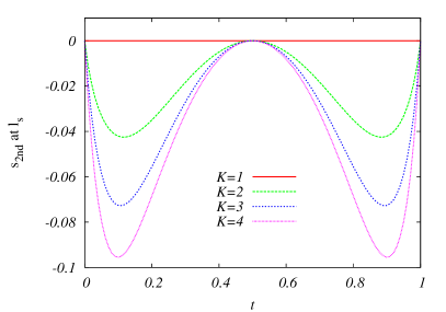
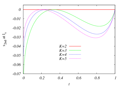
The first and second moment of the number of solutions in the occupation problems has been computed for a general degree distribution in [42]. Based on numerical results it has been also argued non-rigorously in [42] that the above conjecture holds in the balanced locked problems. Here we illustrate that it also holds in the -in- SAT on random -regular graphs for . The first moment entropy, defined by (3), is in the -in- SAT on random -regular graphs given by eq. (14). The second moment entropy is given by where [42]
| (19) |
The interpretation of the parameter follows from expression
| (20) |
where and are configurations and is a probability over the graph ensemble. The parameter in (19) is then the number of sites occupied in both and divided by number of sites occupied in one of the solutions, . We remind that in the -in- SAT the satisfiability threshold is given by cancellation of the entropy (14)
| (21) |
As is a maximum of a function of a single variable , we plot at in Fig. 2. Evaluation of the polynomial function (19) for many values of and in Mathematica shows that for we have , and for we have .
We also investigated numerically general formulas for the second moment presented in [42] and concluded that for , and for , holds also for all the other locked factorized problems.
4.2 Satisfiable factorized locked problems equivalent to the planted ones
We also conjecture that in the factorized locked models the planted ensemble is asymptotically equivalent to the ensemble of satisfiable instances in the whole region of .
For a general (non necessarily locked) constraint satisfaction problem the space of satisfying assignments is separated into clusters. We define the entropy of a cluster as the logarithm of the number of assignments that belong to this cluster. We also define the complexity as the logarithm of the number of clusters of a given entropy . The function is well defined even in the unsatisfiable region: when it then corresponds to the large deviation function for the existence of a cluster of a given size [36]. It was argued in [24] that the cluster containing the planted configuration has a size such that . On the other hand from the large deviation interpretation of the function, most of the rare satisfiable instances in the unsatisfiable region will have one cluster of size .
In the locked problems, all clusters contain a single satisfying assignments, hence for all clusters. Keeping in mind the large deviation interpretation of the complexity [36], the rare satisfiable instances have a single solution and should be asymptotically equivalent to planted instances. And hence the satisfiable and planted ensembles are asymptotically equivalent in the whole range of in the factorized locked problems.
5 Single solution instances
As discussed in the introduction, it is of practical importance to be able to create hard instances which have a single solution with a large probability. Based on the heuristic cavity method results of [24] we conjecture that in the region with high probability there is a single solution on large planted instances of the factorized locked problems (or a couple in case of balanced problems). In this section we prove (assuming the properties of the 1st and 2nd moment from the previous section) this statement for the -in- SAT on random regular graphs. We believe that the generalization of the proof is possible also for the other factorized locked problems.
First note that the first moment in the planted -in- SAT is related in a simple way to the first and second moment in the purely random ensemble. It holds for the entropies
| (22) |
See an example of the function in Fig. 3.
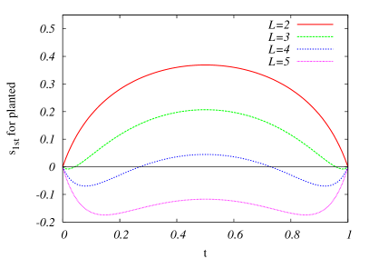
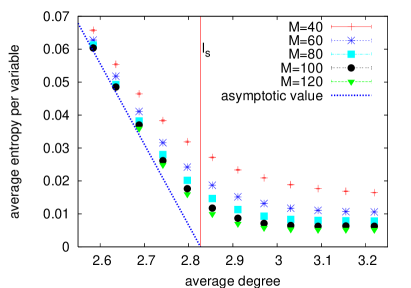
From the previous section it follows that for the first moment entropy in the planted ensemble is a negative function for all . The parameter is in the planted ensemble interpreted as the distance from the planted solution. Therefore, for there are no solutions at an extensive (i.e. ) distance from the planted solution (except the solution at distance one in the balanced problems).
Theorem 11.
Consider a large instance of the -in- SAT problem drawn from the planted ensemble, the degree of variables be . Then there exists an such that with high probability there is no solution at distance smaller than from the planted solution
We will use the expander properties of regular bipartite graphs. The following theorem is well known in the theory of expanders [39].
Theorem 12.
[Sipser and Spielman [39]] Consider a random factor-graph with degree of variables and degree of constraints . Then, for any , there exists a constant , such that with high probability for every set of variables the number of neighboring constraints is larger than . In other words the factor graph is a expander.
of Theorem 11.
Let us prove the statement by contradiction. Suppose that as for every there is a solution at distance smaller that from the planted solution. Denote the distance between the planted and this nearby solution . Now consider the factor-graph and the planted solution, of variables have to be changed to reach the nearby solution. Since can be arbitrarily small Theorem 12 implies that there is at least constraints in which at least one variable has been changed. The property defining a locked constraint is that if a variable is changed then at least one other has to be changed in order to satisfy the constraint again. Hence each of the at least constraints have to be connected by at least two edges to the changed variables. There is hence at least edges connected to changed variables. The total degree of changed variables is , hence . But as can be as near to as we wish this inequality cannot hold and we hence reached a contradiction. This proofs that there exists such that with high probability there is no solution at distance smaller than from the planted one. ∎
Properties of the first moment in the planted ensemble together with Theorem 11 imply that in the planted -in- SAT on random regular graphs there is almost surely a single solution (or a pair of solutions for ).
6 Average computational hardness
One of the most interesting aspects of the study of random constraint satisfaction problems is the average computational hardness of a given ensemble. This has been discussed extensively in both the computer science and the physics literature, in particular for the K-satisfiability and coloring problems. It has been shown empirically that the hardest instances lie very near to the satisfiability threshold , and an easy-hard-easy pattern is often described [5, 31]. Later works focused on predicting up to which connectivity polynomial algorithms are able to find solutions, see e.g. [30, 41, 37]. Instances with a very large density of constraints are typically unsatisfiable. In some problems, e.g. K-satisfiability, no on average polynomial algorithms are known to show unsatisfiability for arbitrary large but constant density of constraints [6]. In other, more constraint, problems unit clause propagation based schemes were shown to be efficient [1]. In the planted instances, which are always satisfiable, it is known that for sufficiently large density of constraints solutions can be found in polynomial time, see e.g. [21, 8]. The situation in the planted factorized locked problems is very interesting: on top of the easy low and high constraint density phases we show that there also exists an intermediate hard phase, and we locate both the boundary thresholds.
We argued that in the satisfiable phase the planted and random ensembles are asymptotically equivalent, this includes the average behavior of algorithms. It was argued in [43, 42] that for average degree the locked problems are algorithmically easy whereas for they are on average hard.
The second hard-easy transition is particular to the planted ensemble and happens in the unsatisfiable phase . We will study the behavior of the BP equations initialized randomly to locate this transition.
6.1 The spinodal point
By definition of the factorized locked problems the belief propagation equations (1) initialized randomly converge to a uniform fixed point. But as the average degree is growing this ceases to be true. In the problems that we are studying here, there actually exists a critical average degree beyond which belief propagation converges spontaneously towards the planted solution. This yields a clear hard-easy transition in the algorithmic complexity. In statistical physics terms this threshold corresponds to a spinodal point of the liquid state [24]. The spinodal point also corresponds to the Kesten-Stigum bound [19, 20], and to the robust reconstruction threshold on trees [16]. This is yet another important connection between the reconstruction problem and the planted ensemble.
In order to compute the spinodal point let us first define matrix . Consider a variable and one of its neighbors, is then the probability that in the planted configuration the variable was assigned given that its neighbors was . In the terms on reconstruction on trees is the probability that in the broadcasting a variable was assigned given its parent was . Components of can be computed as
| (23) | |||
| (24) |
where
| (25) |
where is given by (10) or (11). Explicit formulas for the regular problems are
| (26) | |||
| (27) |
The first eigenvalue of this matrix is equal to one, and is associated with a trivial homogeneous eigenvector. The second eigenvalue of the matrix is given by
| (28) |
A well-known property of the reconstruction on a tree is that reconstruction is always possible beyond the so called Kesten-Stigum (KS) threshold [19, 20]. In our notation the KS condition says that if then the reconstruction is possible, i.e., the leaves asymptotically contain some information about the value sent by the root. In statistical physics the Kesten-Stigum condition is equivalent to the de Almeida-Thouless instability of the paramagnetic phase towards a spin-glass phase [9, 26, 22], that is for the belief propagation equations (1) do not converge. This can be seen from the fact that
| (29) |
where , and .
The eigenvalue and the condition for reconstructibility also appear in the problem of robust reconstruction on trees [16]. In the problem of robust reconstruction it is required that even if an arbitrary large fraction of the values on the leaves is erased there is still information about the root left.
The analysis of the instability of the uniform BP fixed point towards the planted solution then goes as follows. Consider a part of the factor-graph as depicted in Fig. 1. Denote the values of the messages in the uniform fixed BP fixed point by over-bars. Consider the incoming message to be perturbed from the uniform value as
| (30) |
Note that can be both negative or positive. The equation (29) then implies that the outgoing message will be
| (31) |
In other words, any infinitesimal noise in one of the incoming message is multiplied by in the recursion.
We call the perturbation of the incoming message if was occupied in the planted configuration, and otherwise. If the variable was planted in the occupied state, then was planted occupied with probability , and empty with probability . Similarly, if the variable was planted in the empty state, then was planted empty with probability and occupied with probability . Thus the evolution of the perturbation is governed by the equation:
| (32) |
Moreover there are possible incoming messages in the regular graph, thus the criterion . If then the perturbation decreases and we find only the uniform BP fixed point, if on the contrary the uniform BP fixed point is unstable and a perturbation towards the planted configuration amplifies exponentially.
As the planted configuration corresponds to a stable BP fixed point111Note that in the above calculation we considered the stability around the uniform BP fixed point, if we consider the BP fixed point corresponding to the planted solution the perturbation does not amplify. the BP iterations converge instead to the planted solution. Fig. 5 confirms that this is true even on rather small graphs. On the balanced locked problems, where we are not restricted to regular graphs, the correct condition is , where is the mean of the excess degree distribution . The spinodal point , see Tabs. 3,4, is then defined by
| (33) |
for the regular graphs, and
| (34) |
for the truncated Poissonian distribution.
The existence of this spinodal point, together with the conjecture about equivalence between the planted ensemble and the ensemble of satisfiable instances from the random ensemble, Sec. 4, implies that for it is easy to recognize almost all satisfiable instances of the locked problems. Similar conclusions, without a sharp threshold, were established for the coloring and satisfiability problems in [7, 11].
6.2 Belief propagation as a solver
Belief propagation reinforcement is a good solver in the region as shown empirically in [43, 42] in the random ensemble. Since the two ensembles are equivalent in that region, nothing changes for the planted ensemble. We have indeed verified this numerically.
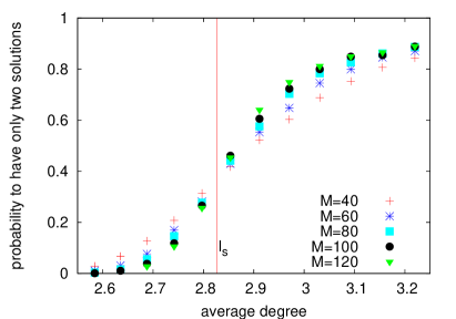
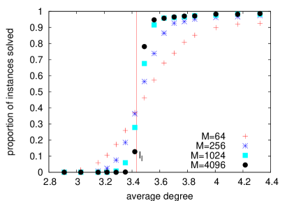
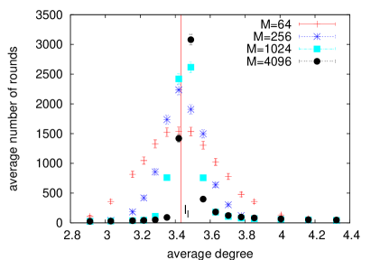
Based on the above arguments, belief propagation equations converge to the uniform fixed point for and directly to the planted solution for . In order to verify that on finite size instances, we have performed the following numerical experiment: we have generated many planted instances for different sizes and average degrees ( instances for each set of parameters). We then iterated the BP equations (1) starting from random initial conditions. For numerical stability reasons we used dumping in the iterations, i.e. each time we computed a new message we kept one half of the sum of the new and old message. As a convergence criterion we used that the messages should not change more that per message (we checked that a smaller criterion does not change the quality of results, and only slows down the computation). This way every iteration converged either to a configuration where the bias of each variable pointed towards the planted solution (or to its negation) or to a point very near to the uniform fixed point. Fig. 5 shows in what fraction of the runs we were able to find the planted solution and in particular it confirms that for it is easy to find it in linear time. On the right of the same figure we plot the average convergence time (given the criterion per message). We see that around the spinodal point the convergence time diverges from both the sides (slightly faster from the large degree side).
7 Conclusions and perspectives
In this work we have studied a class of constraint satisfaction problems on a planted ensemble. The solution is planted in a quiet way, i.e. the planted configuration is one of the typical solutions of the resulting instance. So far we know how to realize such plantings only on the factorized problems. We describe several connections between this quiet planting and the problem of reconstruction on trees.
We study the locked problems because of the simple structure on the space of their solutions — solutions are isolated points instead of clusters. This property makes the locked problems, however, very hard algorithmically. We focused on the class of occupation locked problems in this manuscript, all our results generalize easily to any factorized locked problem, on non-binary variables for example.
On non-locked but factorized problems, as e.g. graph coloring, the concept of quiet planting stays valid [24], however, the random and planted ensembles are not equivalent up to the satisfiability threshold. Moreover, in the unsatisfiable phase the planted ensemble has exponentially many solutions, instead of a single one as is the case in the locked problems. The non-locked problems are also much less friendly for first and second moment considerations. The phase diagram of the locked but non-factorized problem will not be very different from the one presented here. However, the thresholds will be different in the planted and random ensembles and the two ensembles are not equivalent.
One of the most important results of our work is the location of the algorithmically hard region, between , in the problems under investigation. It would be in particular interesting to design an algorithm which would provably find solutions in the region , as we have only heuristic and numerical arguments. This is also challenging in the non-locked problems, as e.g. graph coloring, where we predicted the planted Poisson ensemble to be easy above (on planted regular graphs ), where is the number of colors. Results establishing that the planted ensemble on coloring is easy above , where is some constant quite larger that one, are already known [21, 8].
Finally, another consequence of our work worth discussing is that we know how to generate unique satisfying assignment instances - both in the hard and easy regions. Such instances are often used for evaluating the performance of the quantum annealing algorithm, but so far they have been generated with an exponential cost from an ensemble with unknown classical average computational complexity [40, 12]. In our opinion, these works should be repeated on instances of the locked problems. We conjecture that in the classically hard region also the quantum annealing will be exponential (this is because we anticipate a first order phase transition in the transverse magnetic field, as in [17]).
Acknowledgments
We thank to Dimitris Achlioptas, Amin Coja-Oghlan, Matti Jarvisalo, Andrea Montanari, Cris Moore and Guilhem Semerjian for fruitful discussions and suggestions.
References
- [1] Dimitris Achlioptas, Arthur Chtcherba, Gabriel Istrate, and Cristopher Moore, The phase transition in 1-in-k sat and nae 3-sat, in SODA ’01: Proceedings of the twelfth annual ACM-SIAM symposium on Discrete algorithms, Philadelphia, PA, USA, 2001, SIAM, pp. 721–722.
- [2] Dimitris Achlioptas and Amin Coja-Oghlan, Algorithmic barriers from phase transitions. arXiv:0803.2122v2, 2008.
- [3] S. Ben-Shimon and D. Vilenchik, Message passing for the coloring problem: Gallager meets alon and kahale, in Proceedings of the 13th International Conference on Analysis of Algorithms, DMTCS proc., 2007, pp. 217–226.
- [4] G. Biroli and M. Mézard, Lattice glass models, Phys. Rev. Lett., 88 (2002), p. 025501.
- [5] Peter Cheeseman, Bob Kanefsky, and William M. Taylor, Where the Really Hard Problems Are, in Proc. 12th IJCAI, San Mateo, CA, USA, 1991, Morgan Kaufmann, pp. 331–337.
- [6] Vašek Chvátal and Endre Szemerédi, Many hard examples for resolution, J. ACM, 35 (1988), pp. 759–768.
- [7] A. Coja-Oghlan, M. Krivelevich, and D. Vilenchik, Why almost all k-colorable graphs are easy to color, in Proceedings of the 24th International Symposium on Theoretical Aspects of Computer Science (STACS), LNCS 4393, 2007, pp. 121–132.
- [8] Amin Coja-Oghlan, Elchanan Mossel, and Dan Vilenchik, A spectral approach to analyzing belief propagation for 3-coloring, Combinatorics, Probability and Computing, 18 (2009), pp. 881–912.
- [9] J. R. L. de Almeida and D. J. Thouless, Stability of the Sherrington-Kirkpatrick solution of a spin-glass model, J. Phys. A, 11 (1978), pp. 983–990.
- [10] William Evans, Claire Kenyon, Yuval Peres, and Leonard J. Schulman, Broadcasting on trees and the Ising model, Ann. Appl. Probab., 10 (2000), pp. 410–433.
- [11] R. Monasson F. Altarelli and F. Zamponi, Can rare sat formulas be easily recognized? on the efficiency of message passing algorithms for k-sat at large clause-to-variable ratios, J. Phys. A: Math. Theor., 40 (2007), pp. 867–886.
- [12] E. Farhi, J. Goldstone, S. Gutmann, J. Lapan, A. Lundgren, and D. Preda, A quantum adiabatic evolution algorithm applied to random instances of an np-complete problem, Science, 292 (2001), p. 472.
- [13] U. Feige, E. Mossel, and D. Vilenchik, Complete convergence of message passing algorithms for some satisfiability problems, in Proc. of Random 2006, LNCS 4410, 2006, p. 339–350.
- [14] Robert G. Gallager, Low-density parity check codes, IEEE Trans. Inform. Theory, 8 (1962), pp. 21–28.
- [15] R. G. Gallager, Information theory and reliable communication, John Wiley and Sons, New York, 1968.
- [16] Svante Janson and Elchanan Mossel, Robust reconstruction on trees is determined by the second eigenvalue, Ann. Probab., 32 (2004), pp. 2630–2649.
- [17] Thomas Joerg, Florent Krzakala, Jorge Kurchan, and A. C. Maggs, Simple glass models and their quantum annealing, Phys. Rev. Lett., 101 (2008), p. 147204.
- [18] R. J. Bayardo Jr. and J. D. Pehousek, Counting models using connected components, in Proc. 17th AAAI, Menlo Park, California, 2000, AAAI Press, pp. 157–162.
- [19] H. Kesten and B. P. Stigum, Additional limit theorems for indecomposable multidimensional galton-watson processes, The Annals of Mathematical Statistics, 37 (1966), p. 1463.
- [20] , Limit theorems for decomposable multi-dimensional galton-watson processes, J. Math. Anal. Appl., 17 (1966), p. 309.
- [21] M. Krivelevich and D. Vilenchik, Semi-random models as benchmarks for coloring algorithms, in Proceedings of the Third Workshop on Analytic Algorithmics and Combinatorics (ANALCO), 2006, pp. 211–221.
- [22] Florent Krzakala, Andrea Montanari, Federico Ricci-Tersenghi, Guilhem Semerjian, and Lenka Zdeborová, Gibbs states and the set of solutions of random constraint satisfaction problems, Proc. Natl. Acad. Sci. U.S.A, 104 (2007), p. 10318.
- [23] F. Krzakala, M. Tarzia, and L. Zdeborová, A Lattice Model for Colloidal Gels and Glasses, Phys. Rev. Lett., 101 (2008), p. 165702.
- [24] Florent Krzakala and Lenka Zdeborová, Hiding quiet solutions in random constraint satisfaction problems, Phys. Rev. Lett., 102 (2009), p. 238701.
- [25] F. R. Kschischang, B. Frey, and H.-A. Loeliger, Factor graphs and the sum-product algorithm, IEEE Trans. Inform. Theory, 47 (2001), pp. 498–519.
- [26] Marc Mézard and Andrea Montanari, Reconstruction on trees and spin glass transition, J. Stat. Phys., 124 (2006), pp. 1317–1350.
- [27] M. Mézard and A. Montanari, Information, Physics, Computation, Oxford University Press, Oxford, 2009.
- [28] M. Mézard and G. Parisi, The bethe lattice spin glass revisited, Eur. Phys. J. B, 20 (2001), p. 217.
- [29] M. Mézard, G. Parisi, and M. A. Virasoro, Spin-Glass Theory and Beyond, vol. 9 of Lecture Notes in Physics, World Scientific, Singapore, 1987.
- [30] M. Mézard, G. Parisi, and R. Zecchina, Analytic and algorithmic solution of random satisfiability problems, Science, 297 (2002), pp. 812–815.
- [31] David G. Mitchell, Bart Selman, and Hector J. Levesque, Hard and easy distributions for SAT problems, in Proc. 10th AAAI, Menlo Park, California, 1992, AAAI Press, pp. 459–465.
- [32] A. Montanari and G. Semerjian, On the dynamics of the glass transition on bethe lattices, J. Stat. Phys., 124 (2006), pp. 103–189.
- [33] T. Mora, Géométrie et inférence dans l’optimisation et en théorie de l’information, PhD thesis, Université Paris-Sud, 2007. http://tel.archives-ouvertes.fr/tel-00175221/en/.
- [34] Elchanan Mossel, Reconstruction on trees: Beating the second eigenvalue, Ann. Appl. Probab., 11 (2001), pp. 285–300.
- [35] J. Pearl, Reverend bayes on inference engines: A distributed hierarchical approach, in Proceedings American Association of Artificial Intelligence National Conference on AI, Pittsburgh, PA, USA, 1982, pp. 133–136.
- [36] O. Rivoire, The cavity method for large deviations, J. Stat. Mech., (2005), p. P07004.
- [37] Sakari Seitz, Mikko Alava, and Pekka Orponen, Focused local search for random 3-satisfiability, J. Stat. Mech., (2005), p. P06006.
- [38] Bart Selman, Henry A. Kautz, and Bram Cohen, Local search strategies for satisfiability testing, in Proceedings of the Second DIMACS Challange on Cliques, Coloring, and Satisfiability, Michael Trick and David Stifler Johnson, eds., Providence RI, 1996.
- [39] Michael Sipser and Daniel A. Spielman, Expander codes, IEEE Transactions on Information Theory, 42 (1996), pp. 1710–1722.
- [40] A. P. Young, S. Knysh., and V.N. Smelyanskiy, Size dependence of the minimum excitation gap in the quantum adiabatic algorithm, Phys. Rev. Lett., 101 (2008), p. 170503.
- [41] L. Zdeborová and F. Krzakala, Phase transitions in the coloring of random graphs, Phys. Rev. E, 76 (2007), p. 031131.
- [42] L. Zdeborová and M. Mézard, Constraint satisfaction problems with isolated solutions are hard, J. Stat. Mech., (2008), p. P12004.
- [43] , Locked constraint satisfaction problems, Phys. Rev. Lett., 101 (2008), p. 078702.