Conductance through a potential barrier embedded in a Luttinger liquid:
nonuniversal scaling at strong coupling.

Abstract

We calculate the linear response conductance of electrons in a Luttinger liquid with arbitrary interaction $g_{2}$, and subject to a potential barrier of arbitrary strength, as a function of temperature. We map the Hamiltonian in the basis of scattering states into an effective low energy Hamiltonian in current algebra form. First the renormalization group (RG) equation for weak interaction is derived in the current operator language both using the operator product expansion and the equation of motion method. To access the strong coupling regime, two methods of deducing the RG equation from perturbation theory, based on the scaling hypothesis and on the Callan-Symanzik formulation, are discussed. The important role of scale independent terms is emphasized. The latter depend on the regulaization scheme used (length versus temperature cutoff). Analyzing the perturbation theory in the fermionic representation, the diagrams contributing to the renormalization group $\beta$-function are identified. A universal part of the $\beta$-function is given by a ladder series and summed to all orders in $g_{2}$. First non-universal corrections beyond the ladder series are discussed and are shown to differ from the exact solutions obtained within conformal field theory which use a different regularization scheme. The RG equation for the temperature dependent conductance is solved analytically. Our result agrees with known limiting cases.

I Introduction

The quantum theory of charge transport in one-dimensional (1D) systems of interacting fermions is a fundamental building block of our understanding of electron transport in nanostructures and of a future nanoelectronics. One-dimensional interacting fermion systems have been studied since the 1950s, beginning with the pioneering works of Tomonaga and Luttinger. The early work exploited the fact that the elementary excitations in these systems are charge and spin excitations of bosonic character, and led to the formulation of the method of bosonization. GoNeTs ; GiamarchiBook This method offers a natural description of the fractionalization of the usual fermionic quasiparticles existing in higher dimensions, into spinon and holon quasiparticles in 1D. While the bosonization method is highly successful in accounting for the properties of systems in equilibrium, it is somewhat problematic when applied to transport situations. For example, an ideal quantum wire attached to two reservoirs is expected to have a two-point conductance of $R_{Q}=\frac{e^{2}}{h}$ per channel. In contradiction to this general law it was found in early work on transport in clean Luttinger liquids Apel1982 ; Kane1992 ; Kane1992a that the conductance (here and in the following conductance will be measured in units of the conductance quantum $R_{Q}$) is given by the Luttinger parameter $K$, and thus depends on the interaction strength. It was later pointed out that by carefully choosing the order of limits of frequency, $\omega\rightarrow 0$, and wire length, $L\rightarrow\infty$, Maslov1995 ; Safi1995  or else by taking into account the screening of the external field by the interacting electron system Oreg1996  one recovers the correct value of unity for the two-point conductance. Whether the former or the latter explanation is the correct one remains disputed to this day.

The more relevant case of a Luttinger liquid with potential barrier has been considered first by Kane and Fisher Kane1992 ; Kane1992a and by Furusaki and Nagaosa, Furusaki1993 again using the bosonization method. These authors found that interaction has a dramatic effect on the conductance: for repulsive interaction the conductance is found to tend to zero as a fractional power of the temperature $T$ , in the limit $T\rightarrow 0$ . This was shown in the two limits of a weakly scattering barrier and a strong (tunneling) barrier. In addition, results in the complete temperature range are available at special values of the interaction parameter, $K=\frac{1}{2}$ and $K=\frac{1}{3}$. Kane1992 ; Kane1992a ; Weiss1995 ; Fendley1995 ; Fendley1995a All these works suffer from the drawback that in the clean limit the conductance is found to tend to $K$ rather than $1$ . It has been argued that these results may be applied to the four-point conductance. However, the four-point conductance is expected to tend to infinity in the limit of vanishing barrier strength, a behavior not shown.

For the reasons noted above we think it worthwhile to develop an alternative formulation of the transport theory of Luttinger liquids, formulated entirely in the fermionic language. The fermionic representation offers the possibility to connect the fermionic degrees of freedom in the (non-interacting) leads smoothly with the degrees of freedom in the interacting system. In other words, it allows to use the scattering states of the system in the non-interacting limit as a basis of description. On the simplest level, in lowest order in the interaction, this program has been carried out in a seminal paper by Yue, Matveev and Glazman. Yue1994 The physics of this problem lies in the scale-dependent build-up of a polarization potential around the bare barrier, induced by the Friedel oscillations of the density. For repulsive interaction, the polarization potential is found to extend farther and farther out as the temperature is lowered, until at $T=0$ it is infinitely extended, leading to a vanishing transmission probability across the barrier. The process of gradual growth of the effective potential barrier may be described in the language of renormalization group theory applied to the transmission probability as a function of the temperature. A generalization of the approach of Yue et al. to the case of two barriers has been given in Ref. [Polyakov2003, ]. These predictions, based on the continuum version of the theory, were thoroughly checked and confirmed by the fermionic functional renormalization group method, starting from the Hubbard models on a lattice. Enss2005 ; Andergassen2006

In this paper we report on a significant extension of the work of Yue et al. to the case of systems of spinless fermions in 1d interacting via arbitrarily strong forward scattering (parameter $g_{2}$) and subject to a short range barrier potential (width $a$). The principal tool we will be using is perturbation theory in the interaction, summed to infinite order. To achieve this goal, and to gain insight into the structure of perturbation theory, we map the problem first onto an effective model of interacting currents of chiral fermions. The reformulation allows to describe the effect of the barrier potential as a local magnetic field at the position of the barrier, acting on the pseudospin vector of the chiral current. The logarithmic corrections to this field, stemming from the fermionic interactions can be addressed in a simplified poor-man scaling approach; however this approach becomes ambiguous in higher orders. Therefore at a later stage we will apply the Callan-Szymanzik type of analysis, by first introducing the counter terms to magnetic field part of the Hamiltonian to compensate the effect of the interaction, and secondly requiring the “bare” value of the field to be independent of the high-energy cutoff. Equivalently, we may assume the scaling property of the conductance to hold, entailing the existence of a renormalization group equation for the conductance as a function of the scaling variable $\Lambda$ (at finite temperature $\Lambda=\ln(T_{0}/T)$ ). By comparison with the structure of perturbation theory for the conductance, which is given by a power series in the interaction and in the scaling parameter $\Lambda$ , one may extract the RG $\beta$-function. In this way we derive a universal renormalization group equation for the conductance as a function of the scaling parameter.

The most important consequence of the current algebra formulation is, however, to allow for an efficient organization of perturbation theory. After presenting the formulation of perturbation theory as well as a few low order results we analyze the structure of the perturbation expansion with respect to logarithmically divergent terms containing powers of  $\Lambda=\ln(L/a)$  or  $\ln(T_{0}/T)$. We identify a class of universal diagrams contributing the principal terms linear in $\Lambda$ and derive an integral equation resumming these contributions (“ladder approximation”). These terms are shown to dominate in both limits, small and large conductance. We identify the prefactor of the terms in the perturbation series for the conductance $G$ linear in $\Lambda$ with the renormalization group $\beta$-function of the flow equation of $G(\Lambda)$. There is, however, one important new feature: there appear scale independent terms (from third order on), which lead to a correction of the conductance even at $\Lambda=0$, the ultraviolet cutoff. These terms must be taken into account, in order to preserve the scaling property of the conductance, and lead to a starting value of the conductance $G(\Lambda=0)$, different from the conductance in the absence of interaction.

The RG equation may be solved analytically in the ladder approximation, to give the conductance as a function of temperature for any interaction strength and barrier potential. The result completely agrees with earlier work, where a comparison is appropriate We emphasize that our result for the conductance reduces to unity in the absence of a barrier. Furthermore, the effect of screening of the external field Oreg1996   is included by omitting all polarization diagrams. We checked the renormalizability of the theory explicitly by calculating all terms up to third order in $\Lambda$ and $g_{2}$ .

At intermediate temperatures (semi-transparent barrier) additional diagrams contribute small corrections to the $\beta$-function. We calculate these terms in lowest (third) order in $g_{2}$ . A proper treatment of these contributions requires taking into account scale independent terms in a way sketched above. We demonstrate explicitly that the resulting $\beta$-function is uniquely determined for a given physical quantity. However, $\beta$ turns out to be a slightly different function for the two cases of interest here, the temperature dependent and the length dependent conductance. The result of the solution of the RG-equation for the conductance, using the approximate $\beta$-function thus obtained, is found to agree quantitatively with all known results on the scaling behavior of the conductance in the limits $G\rightarrow 0$ and $G\rightarrow 1$ . In the intermediate regime $G\sim 1/2$ we find small discrepancies with the results of conformal field theory in the case $K=\frac{1}{2}$, which we can trace back to a different cutoff scheme used there and the effect of higher order terms neglected in our work. As an excellent interpolation formula between two exact limits our result goes beyond all previous works: it is valid for any interaction strength $K$ and any potential scattering strength.

I.1 Formulation of the problem

The Hamiltonian includes the kinetic energy of freely right- and left-moving (R,L) spinless fermions with linearized dispersion, $H_{0}$, the interaction energy between the left- and right-moving densities, $H_{1}$, and the impurity part decribing scattering off the barrier, placed at the origin, $H_{imp}$ :

$$H = H_{0}+H_{1}+H_{imp}$$ (1)

$$H_{0} = v_{F}\int_{-\infty}^{\infty}{dx}\left[\psi_{R}^{\dagger}(i\partial_{x})\psi_{R}-\psi_{L}^{\dagger}(i\partial_{x})\psi_{L}\right]$$

$$H_{1} = g_{2}\int_{-L}^{L}{dx}\;(\psi_{R}^{\dagger}\psi_{R})(\psi_{L}^{\dagger}\psi_{L})$$

In order to regularize the theory, we assume that the region of interaction $|x|>a$, where $g_{2}\neq 0$, and the region over which the impurity potential is nonzero, $|x|<a\sim k_{F}$ ($k_{F}$is the Fermi wave vector) do not overlap spatially. The length scale $a$ will serve as an ultraviolet cutoff in the scale dependent logarithmic corrections considered below.

The last term, $H_{imp},$ in (1) is not explicitly specified here (but see below). We will rather take the one-particle scattering states to be known. This means that we characterize the barrier by transmission and reflection amplitudes $t=\tilde{t}=\cos\theta$, $r=-\tilde{r}^{\ast}=i\sin\theta e^{i\phi}$ , with negligible energy dependence in the energy range of interest (here $t$, $\tilde{t}$, $r$, $\tilde{r}$ are the usual components of the impurity scattering matrix). Notice also that we assume the system to be non-interacting in the leads, $|x|>L$, which allows for an asymptotic single-particle scattering states representation.

We define the creation operator of scattering states as

$$\psi_{k}^{{\dagger}}(x) = (e^{ikx}+r_{k}e^{-ikx})c_{1k}^{\dagger}+\tilde{t}_{k}e^{-ikx}c_{2k}^{\dagger},\quad x<0$$ (2)

$$= t_{k}e^{ikx}c_{1k}^{\dagger}+(\tilde{r}_{k}e^{ikx}+e^{-ikx})c_{2k}^{\dagger},\quad x>0$$

with $c_{1k}^{\dagger}$ ($c_{2k}^{\dagger}$) the creation operators of asymptotically right-going (left-going) fermions of momentum $k$. Such a representation requires the kinetic energy part of the Hamiltonian to be of the form $-\nabla^{2}/(2m)$, and the momentum, $k=\sqrt{2mE}>0$, before the linearization of the dispersion around the two Fermi points. In appendix A we clarify the correspondence between the scattering states representation (2) and our linearized Hamiltonian (1) written in the basis of chiral fermions.

For simplicity we do not consider the so-called $g_{4}$ part of the fermionic interaction in this work, i.e. the term $\frac{1}{2}g_{4}\int_{-L}^{L}{dx}\;[(\psi_{R}^{\dagger}\psi_{R})^{2}+(\psi_{L}^{\dagger}\psi_{L})^{2}]$. For $L\rightarrow\infty$ the $g_{4}$-interaction can be absorbed into the redefinition of the Fermi velocity, $\tilde{v}_{F}=v_{F}+g_{4}/2\pi$. For finite $L$ one can show that $g_{4}$ does not lead to a renormalization of d.c. conductance, which is the quantity of interest below. The effect of $g_{4}$ on the a.c. conductance can be analyzed, following the guidelines in Oreg1995 ; Safi1995 .

It appears that in the case of weak potential scattering, $U(x)\ll E_{F}$, and for electrons with energies close to the Fermi energy, $E_{F}$, the situation is characterized two limits of the Fourier transform $U(q)$ of the potential: the forward scattering amplitude, $U(q\simeq 0)=u_{1}$, and the backward scattering amplitude, $U(q\simeq 2k_{F})=u_{2}$, with real-valued $u_{1}$ and complex-valued $u_{2}$. The fermionic Hamiltonian $H_{imp}$ in (1) is then written as

$$H_{imp} = v_{F}\int{dx}\left[u_{1}(x)(\psi_{R}^{\dagger}\psi_{R}+\psi_{L}^{\dagger}\psi_{L})\right.$$

$$\left.+(u_{2}(x)\psi_{L}^{\dagger}\psi_{R}+h.c.)\right],$$

where the dimensionless functions $u_{1,2}(x)$ are short-range impurity potentials, which means that $u_{1,2}(x)=0$ for $|x|>a$ and the above amplitudes $u_{1,2}=\int dx\,u_{1,2}(x)$.

In Appendix A we show that the connection between the microscopic Hamiltonian and the $S$-matrix can be clarified in some simple cases, but requires a detailed knowledge of $u_{1,2}(x)$, when one goes beyond the lowest Born approximation.

Returning to (2), we define Fourier transforms, $\psi_{1}^{+}(x)=\int_{0}^{\infty}\frac{dk}{2\pi}e^{ikx}\tilde{c}_{1,k}^{+}$ and $\psi_{2}^{+}(x)=\int_{0}^{\infty}\frac{dk}{2\pi}e^{-ikx}\tilde{c}_{2,k}^{+}$. Then we have for the electron creation operator at position $x$

$$\psi^{+}(x) = \left\{\Theta(-x)\left[\psi_{1}^{+}(x)+r\psi_{1}^{+}(-x)+\tilde{t}\psi_{2}^{+}(x)\right]\right.$$ (4)

$$+ \left.\Theta(x)\left[t\psi_{1}^{+}(x)+\tilde{r}\psi_{2}^{+}(-x)+\psi_{2}^{+}(x)\right]\right\}\,,$$

with the step function $\Theta(x)=1$ at $x>0$.

II Interacting case, previous works

II.1 Boundary sine-Gordon model

In bosonization technique, the chiral fermions are represented as exponentials of chiral boson fields, $\psi_{R}^{\dagger}\sim e^{-i\varphi_{R}}$, $\psi_{L}^{\dagger}\sim e^{i\varphi_{L}}$. with the fields $\varphi_{R(L)}=\varphi\mp\theta$. Here the primary field $\varphi$ and its canonically conjugate momentum $\Pi=\pi^{-1}\partial_{x}\theta$ obey the commutation relation $[\varphi(x),\Pi(y)]=i\delta(x-y)$. We have for the density $\psi_{R}^{\dagger}\psi_{R}+\psi_{L}^{\dagger}\psi_{L}=\partial_{x}\varphi/\pi$ and the Hamiltonian (1), (I.1) can be represented as

$$H = \frac{\tilde{v}_{F}}{2\pi}\int dx\Big{[}K\,(\partial_{x}\theta)^{2}+K^{-1}(\partial_{x}\varphi)^{2}$$ (5)

$$+2u_{1}(x)\partial\varphi(x)+u_{2}(x)\cos 2\varphi(x)\Big{]}$$

One has $\tilde{v}_{F}=v_{F}$ and $K=1$ for free fermions, whereas the short-range interaction $H_{1}$ between the fermions, Eq. (1), leads to the renormalized Fermi velocity $\tilde{v}_{F}=v_{F}(1-g^{2})^{1/2}$ and the Luttinger parameter $K=[(1-g)/(1+g)]^{1/2}$. Here and below we use

$$g=g_{2}/(2\pi v_{F})$$ (6)

One usually argues, that the term $u_{1}$ can be absorbed into a redefinition of $\varphi(x)\rightarrow\varphi(x)+u_{1}sgn(x)$ (cf. Appendix A). After this redefinition one concentrates on the $u_{2}$ term which constitutes the boundary sine-Gordon (BSG) problem. A solution to this problem, in the lowest order of $u_{2}$ was presented in the early work. Kane1992 ; Kane1992a Focussing on the small-energy sector of the problem, one uses the renormalization group approach, removing the higher energy states of the problem while simultaneously rescaling the parameters of the action. It turns out that under this procedure the amplitude of the BSG term is renormalized as

$$u_{2}\rightarrow u_{2}e^{(1-K)\Lambda}$$ (7)

where the RG scaling variable $\Lambda=\ln E_{F}/\epsilon>0$ . As a result, the conductance at small $u_{2}$ , given by $G=|t|^{2}\simeq 1-u_{2}^{2}$ , undergoes a similar renormalization

$$G\simeq 1-|u_{2}|^{2}e^{2(1-K)\Lambda}$$ (8)

with the lower cutoff in $\Lambda$ defined by temperature or voltage bias, $\Lambda=\ln E_{F}/\max[T,V]$. We shall confine ourselves to the the linear response regime, $V\ll T$  in the following.

For repulsive interaction $K<1$ the conductance decreases with falling temperature. When the renormalized impurity potential becomes strong, $|u_{2}|^{2}e^{2(1-K)\Lambda}\sim 1$, the weak-impurity assumption is violated and one should use a different line of reasoning. One may think of two semi-infinite parts of the wire, connected by a weak tunneling link $t$. An appropriate RG treatment shows that the repulsive interaction leads to a further decrease of the conductance, which acquires the form

$$G\simeq|t|^{2}e^{2(K^{-1}-1)\Lambda}$$ (9)

These two regimes, Eqs. (8), (9) show different scaling exponents, which are approximately equal for small interaction

$$1-K\simeq K^{-1}-1\simeq g.$$

A smooth crossover between the two asymptotes (8) and (9) was first explicitly provided for a special case of interaction strength, $K=1/2$, which is known as Luther-Emery refermionization point. The full curve for the conductance was obtained Kane1992 ; Kane1992a ; Weiss1995 in the form of a one-parameter scaling function.

In subsequent works Fendley1995 ; Fendley1995a the BSG model was analyzed at arbitrary values of Luttinger parameter, $K$. The set of coupled integral equations was shown to be finite for $1/K=1,2,3\ldots$ and the solution for $K=1/3$ was derived, in particular. Corresponding scaling functions for the conductance were obtained for finite $T$ and voltage bias on the contact $V$ either by numerical solution of the corresponding integral equation or as a series in powers of the scaling parameter, see also Weiss1996 . For practical purposes this form of representation is not very convenient.

In principle, the statement of a one-parameter scaling function for the conductance and the knowledge of its actual form provides a solution for the temperature renormalization of the barrier apparently at arbitrary strength. However, it was noted in Fendley1995 ; Fendley1995a , that ”the strong-barrier problem which is at the end of our renormalization-group trajectory follows formally from dimensional continuation of the integrals for the weak barrier problem. It is not in any case a generic strong-barrier problem.”

II.2 Fermionic approach, RG for S-matrix

Yue, Matveev and Glazman Yue1994 have developed a theory, starting from the formalism of scattering states and taking into account the fermionic interaction in lowest order of perturbation. They arrived at the RG equation for the transmission amplitude $t$ in the form

$$\frac{dt}{d\Lambda}=-gt(1-|t|^{2})$$ (10)

The solution to this equation is found as

$$t = \frac{t_{0}}{(|t_{0}|^{2}+(1-|t_{0}|^{2})e^{2g\Lambda})^{1/2}}$$ (11)

which, in leading order in $g$, agrees with Eqs. (8), (9).

The advantage of this approach is its applicability for arbitrary strength of impurity potential. One may thus avoid the step involving the transition from the initial Hamiltonian (5) to the observed conductance, which as we saw above can depend on the short-distance (ultraviolet) details of relevant quantities. This view is further corroborated by the work by Callan et al. Callan1994 who discussed the solution of the non-interacting ($K=1$) BSG theory, and arrived at a current algebra formulation similar to our formulation below. These authors show that the connection of the initial model (5) to the observable quantities depends on the ultraviolet regularization. We will return to this point in our discussion below.

III Scattering states and current algebra

In the above we defined a scattering states representation (4) in chiral representation. In order to describe the effects of interaction, we need to define fermionic densities in the same basis. One may form four bilinear density combinations out of two chiral fermions. It is convenient to group these combinations into chiral densities or “currents”, according to

$$\widehat{J}(x) = \begin{pmatrix}\psi^{\dagger}_{1}(x)\psi_{1}(x)&\psi^{\dagger}_{1}(x)\psi_{2}(-x)\\ \psi^{\dagger}_{2}(-x)\psi_{1}(x)&\psi^{\dagger}_{2}(-x)\psi_{2}(-x)\end{pmatrix}$$ (12)

$$\equiv \begin{pmatrix}J_{0}+J_{3}&J_{1}-iJ_{2}\\ J_{1}+iJ_{2}&J_{0}-J_{3}\end{pmatrix}$$ (13)

We call $J_{0}$ the pseudocharge current and the vector $\vec{J}=(J_{1},J_{2},J_{3})$ the pseudospin current. These operators obey $U(1)$ and $SU(2)$ Kac-Moody algebras, respectively GoNeTs ; Affleck1991 , as we discuss below.

The particle density operators for incoming $(i)$ and outgoing $(o)$ particles in terms of the $J_{\mu}$’s are given by (here and in the following $x>0$ )

$$\rho_{iR}(-x) = \psi_{1}^{\dagger}(-x)\psi_{1}(-x)=J_{0}(-x)+J_{3}(-x)$$ (14)

$$\rho_{iL}(x) = \psi_{2}^{\dagger}(x)\psi_{2}(x)=J_{0}(-x)-J_{3}(-x)$$ (15)

$$\rho_{oR}(x) = (t\psi_{1}^{\dagger}(x)+\tilde{r}\psi_{2}^{\dagger}(-x))(t^{\ast}\psi_{1}(x)+\tilde{r}^{\ast}\psi_{2}(-x))$$ (16)

$$= (S.\widehat{J}(x).S^{\dagger})_{11}=J_{0}(x)+\widetilde{J}_{3}(x)$$

$$\rho_{oL}(-x) = (r\psi_{1}^{\dagger}(x)+\tilde{t}\psi_{2}^{\dagger}(-x))(r^{\ast}\psi_{1}(x)+\tilde{t}^{\ast}\psi_{2}(-x))$$ (17)

$$= (S.\widehat{J}(x).S^{\dagger})_{22}=J_{0}(x)-\widetilde{J}_{3}(x)$$

Here $\widetilde{J}_{3}=(R\vec{J})_{3}$ is the third component of the pseudospin current vector $\vec{J}$ rotated by the orthogonal matrix $R_{\mu\nu}$ given by

$$R_{\mu\nu}=\frac{1}{2}Tr[\sigma_{\mu}.S.\sigma_{\nu}.S^{\dagger}].$$ (18)

with Pauli matrices $\sigma_{\mu}$. It is seen from (18) that the global phase of $S$ drops out completely. Omitting this phase, we parametrize

$$S=\begin{pmatrix}t&\tilde{r}\\ r&\tilde{t}\end{pmatrix}=\begin{pmatrix}\cos\theta&i\sin\theta e^{-i\phi}\\ i\sin\theta e^{i\phi}&\cos\theta\end{pmatrix}$$ (19)

In this notation, the components of interest below read $R_{33}=|t|^{2}-|r|^{2}=\cos 2\theta$, $R_{32}=\mbox{Im}\{t\widetilde{r}^{\ast}+\widetilde{t}r^{\ast}\}=-\sin 2\theta\cos\phi$, and $R_{31}=\mbox{Re}\{t\widetilde{r}^{\ast}-\widetilde{t}r^{\ast}\}=\sin 2\theta\sin\phi$.

We see that the description of the barrier is given by the eigenmodes of the current $J_{i}(x)$, with negative and positive $x$ and $i=0,\ldots,3$. In this picture, the incoming current is given by the diagonal components of the $\widehat{J}$ matrix, and the outgoing currents correspond to the diagonal components of the rotated matrix $S.\widehat{J}.S^{\dagger}$. Evidently, the pseudocharge component $J_{0}$ is not affected by this rotation.

III.1 Formal identities and Green’s functions

The chiral densities introduced above satisfy the Kac-Moody commutation rules

$$[J_{0}(x),J_{0}(y)] = \frac{i}{4\pi}\partial_{x}\delta(x-y)$$ (20)

$${}[J_{j}(x),J_{k}(y)] = \frac{i}{4\pi}\delta_{jk}\partial_{x}\delta(x-y)+i\varepsilon_{jkl}J_{l}(y)\delta(x-y)$$

with $j,k,l=1,\ldots 3$ and totally antisymmetric $\varepsilon_{jkl}$. The short-distance operator product expansions (OPEs) are

$$J_{0}(x)J_{0}(y) = \frac{-1}{8\pi^{2}}\frac{1}{(x-y-i0)^{2}}\,,$$

$$J_{j}(x)J_{k}(y) = \frac{-1}{8\pi^{2}}\frac{\delta_{jk}}{(x-y-i0)^{2}}+\frac{1}{2\pi}\frac{\varepsilon_{jkl}J_{l}(y)}{x-y-i0}\,.$$ (21)

In simple terms, relevant to our discussion below, one can consider (20) as a consequence of (21). In their turn, the OPEs (21) simply represent fermionic Green’s functions, $[2\pi(x-y)]^{-1}$. A bilinear form in the currents is a product of four fermion operators; the complete convolution of these gives a product of two two-point Green’s function (modulo normally ordered operators), and the partial convolution produces a Green’s function multiplied by bilinear forms in the fermion operators, i.e. current operators. The position argument of the latter current operators (last term in (21)) is subject to ambiguity, but usually this concerns only less relevant terms. In our analysis below we deal with an action non-local in the currents, and to handle such an ambiguity becomes an increasingly difficult matter. This is why we resort to the perturbative treatment in terms of chiral fermions.

III.2 Observable current and conductance

The physical charge density is $\rho(x)=\rho_{iR}(x)+\rho_{oL}(x)$ at $x<0$ and $\rho(x)=\rho_{oR}(x)+\rho_{iL}(x)$ at $x>0$. A simple calculation shows that

$$\rho(x) = \rho_{c}(x)+\rho_{s}(x),$$

$$\rho_{c}(x) = J_{0}(-x)+J_{0}(x),$$ (22)

$$\rho_{s}(x) = sign(x)\left(-J_{3}(-|x|)+\widetilde{J}_{3}(|x|)\right).$$

The physical current operator is also decomposed into two parts, in the pseudocharge and pseudospin sectors. We use the continuity equation $-\partial_{x}j(x)=\partial_{t}\rho(x)=-i[\rho(x),H]$ to obtain

$$j(x) = j_{c}(x)+j_{s}(x),$$

$$j_{c}(x) = v_{F}(-J_{0}(-x)+J_{0}(x)),$$ (23)

$$j_{s}(x) = v_{F}(J_{3}(-|x|)+\widetilde{J}_{3}(|x|)),$$

It follows then that the pseudocharge current corresponds to the part of physical density which is even with respect to the reflection at the scatterer, $\rho_{c}(-x)=\rho_{c}(x)$. The pseudospin current corresponds to the odd part of the density, $\rho_{s}(-x)=-\rho_{s}(x)$. This symmetry property simplifies the discussion of a voltage bias, applied to the barrier. One sees immediately, that applying the same electrochemical potential to both leads of the wire corresponds to its coupling to the pseudocharge current. It results in an overall increase of the fermionic density, symmetric with respect to the barrier, and not to a net physical current. By contrast, an electric potential of the form $V(x)=\frac{1}{2}V\,sign(x)$, couples only to the pseudospin part, leading to a term in the Hamiltonian

$$H_{V}=V\int_{0}^{\infty}dx\,(\widetilde{J}_{3}(x)-J_{3}(-x))$$

The physical current induced by a bias voltage is therefore given in linear response theory as

$$\langle j(x,\omega)\rangle = G(x,\omega)V(\omega)$$

$$G(x,t) = -i\Theta(t)\langle[j_{s}(x,t),\int_{0}^{\infty}dy\,\rho_{s}(y,0)]\rangle$$ (24)

A remark is in order here. Strictly speaking, the prefactor $v_{F}$ in the definition (23) applies for non-interacting leads. In the interacting region we have to replace $v_{F}\rightarrow v_{F}-g_{2}/2\pi$ in (23). We may avoid this complication, analyzed elsewhere Oreg1995 ; Safi1995 , by assuming in (24) that both $j_{s}(x,t)$ and $\rho_{s}(y,0)$ are placed outside the interacting region, $x,y>L$. The change of the limits of integration over $y$ in (24) is not important in the limit of d.c. conductance $|\omega|\ll v_{F}/L$, considered below.

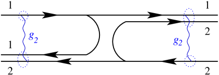
(a) (b)

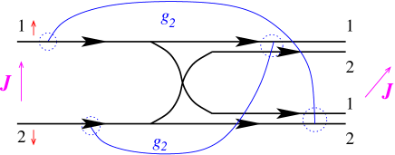
Figure 1: (Color online) (a)The interaction of the left- and right-going densities in the basis of scattered waves. (b) The interaction of the left- and right-going densities in the chiral basis, corresponding to non-local interaction, Eq. (26).

III.3 Hamiltonian

It is known that fermions with linearized dispersion in one spatial dimension can be described by a Hamiltonian, quadratic in chiral fermionic densities. This observation, usually attributed to Tomonaga, is the basis of the bosonization approach. GoNeTs Similarly to (5), we have

$$H_{0}=\pi v_{F}\int_{0}^{\infty}dx(\rho_{iR}^{2}(-x)+\rho_{iL}^{2}(x)+\rho_{oR}^{2}(x)+\rho_{oL}^{2}(-x))$$

which can be represented as

$$H_{0} = 2\pi v_{F}\int_{-\infty}^{0}dx\,(J_{0}^{2}(x)+J_{3}^{2}(x))$$

$$+2\pi v_{F}\int_{0}^{\infty}dx\,(J_{0}^{2}(x)+\widetilde{J}_{3}^{2}(x))$$

The interaction part is

$$H_{1} = g_{2}\int_{a}^{L}dx\,(\rho_{iR}(-x)\rho_{oL}(-x)+\rho_{oR}(x)\rho_{iL}(x))$$ (26)

$$= 2g_{2}\int_{a}^{L}dx\,(J_{0}(-x)J_{0}(x)-J_{3}(-x)\widetilde{J}_{3}(x))$$

In Fig. 1 we show in a pictorial way our parametrization of the fermionic densities and the interaction, $H_{1}$. In Fig. 1a the $g_{2}$-interaction processes are shown in the usual scattering configuration. The representation in terms of the chiral currents $J_{\mu}$ (all particles moving to the right) is shown in Fig. 1b and leads to a seemingly nonlocal interaction. Notice that in the case of perfect reflection, $t=0$, we have $\tilde{J}_{3}=-J_{3}$ and the observable densities (see below) form an Abelian $U(1)$ sub-algebra of $SU(2)$. This case of “open boundary bosonization”, considered by Fabrizio and Gogolin, allows a complete and rather simple analysis Fabrizio1995 . In the next subsection we elucidate what happens at the origin, $x=0$. .

III.4 The barrier as magnetic field

Using the parametrization (19), one finds that $R_{ij}=\exp(\varepsilon_{ijk}B_{k})$ i.e., it is a finite rotation characterized by the dual vector $\mathbf{B}=2\theta(\cos\phi,\sin\phi,0)$. We cannot symmetrize the Hamiltonian in the pseudospin space, reducing it to the so-called Sugawara form, GoNeTs because the vector $\mathbf{B}$ breaks the $SU(2)$ symmetry of the problem. We may symmetrize the Hamiltonian in the plane perpendicular to $\mathbf{B}$, but that provides little advantage .

The above formulation of the problem, incorporating the knowledge about the scatterer in the asymptotic scattering states, is equivalent to the the alternative formulation of the pseudospin current being rotated by a fictitious magnetic field $\mathbf{B}$ located at the origin. The pseudocharge sector remains unchanged and the pseudospin sector of the problem can be equivalently described by the following Hamiltonian

$$H^{\prime} = \int_{-\infty}^{\infty}dx\,\left({2\pi}v_{F}O_{3}^{2}(x)-g_{2}O_{3}(-x)O_{3}(x)\right.$$ (27)

$$\left.+v_{F}B_{j}O_{j}(x)\delta(x)\right),$$

where the operators $O_{j}(x)\equiv U^{\dagger}J_{j}(x)U$, with $j=1,2,3$ obey Kac-Moody relations (20). The two Hamiltonians, (III.3), (26) and (27), are connected by a canonical transformation $H^{\prime}=U^{\dagger}HU$ , where

$$U=\exp i\int_{0}^{\infty}dxB_{j}J_{j}(x).$$

We derive the relation between $O_{j}(x)$ and $J_{j}(x)$ in Appendix B.

Equation (27) resembles the Hamiltonian for the Kondo problem in the current algebra representation. Affleck1991 However there are important differences. The first one is the non-local interaction $g_{2}$ between the incoming and outgoing waves in our case. The second difference is the classical nature of the field $\mathbf{B}$, as opposed to the quantum nature of the Kondo spin $\mathbf{S}$.

The matrix Green’s function for chiral fermions is diagonal in pseudospin space when defined in terms of the asymptotic eigenstates. However in terms of the usual right- and left-movers its matrix structure is evidently given by Eq. (19), which shows the action of the magnetic field $S=\exp i\bm{sB}$, with $\bm{s}=\frac{1}{2}\bm{\sigma}$. We will use this fact in Sec. VI below.

IV RG equation for $S$-matrix

Let us show how the renormalization group equation for the many-body $S-$matrix is simply reproduced in the current operator formalism. Following Affleck and Ludwig, Affleck1991 we write the $g_{2}$ term of the $S-$matrix in the interaction representation as

$$T_{t}\exp 2ig_{2}\int dt\int_{a}^{L}dxJ_{3}(-x)(\widehat{R}J)_{3}(x)$$

Expanding the latter object in first power of $g_{2}$, we find at given $t$

$$-2g_{2}\int_{a}^{L}dxJ_{3}(-x)R_{3j}J_{j}(x)$$

Applying OPE rules (21) to the last expression one finds an operator term

$$J_{3}(-x)J_{j}(x)\sim\frac{\varepsilon_{3jk}}{2\pi}\frac{J_{k}(0)}{-2x}$$

After eliminating the distances close to the scatterer, i.e. integrating over $x$ from $a$ to a certain $a^{\prime}$, which serves now as new lower cutoff, we obtain the term which can be re-exponentiated to the action giving a contribution of the form $\delta H=v_{F}\,\delta B_{k}\,J_{k}(0)$, with

$$\delta B_{k}=\varepsilon_{3jk}R_{3j}\frac{g_{2}}{2\pi v_{F}}\int_{a}^{a^{\prime}}\frac{dx}{x}.$$

We notice further that $\varepsilon_{3jk}R_{3j}\equiv\widetilde{B}_{k}=\sin 2\theta(\cos\phi,\sin\phi,0)$, i.e., the additional magnetic field at the origin is parallel to the above $\mathbf{B}$, and we may restrict the discussion to the change in modulus, $B\rightarrow B+\delta B$. Denoting $d\Lambda=\int_{a}^{a^{\prime}}{dx}/{x}$, we obtain ${d(2\theta)}/{d\Lambda}=g\sin 2\theta$, or

$$\frac{d\,\sin^{2}\theta}{d\Lambda}=2g\sin^{2}\theta\cos^{2}\theta$$ (28)

which is equivalent to Eq. (10).

After this verification of the previous result in the first order in $g$, we are tempted to obtain the next-order corrections to the RG equation (28). It turns out however that working entirely in the current operator formalism gives no advantage in such analysis, as we explain in the next subsection.

IV.1 Higher orders in current operator formalism

Let us return to the last term in (21)

$$J_{j}(x)J_{k}(y)\sim\frac{\varepsilon_{jkl}J_{l}(y)}{2\pi(x-y)}.$$

Using the definition (12), and free fermionic Green’s functions, one obtains e.g. the precise relation

$$J_{2}(x)J_{3}(y)=\frac{\psi_{1}^{\dagger}(x)\psi_{2}(-y)+\psi_{1}^{\dagger}(y)\psi_{2}(-x)+h.c.}{8\pi(x-y)},$$ (29)

modulo the normal ordered part. Evidently, the numerator in (29) is reduced to $4J_{1}(y)$ only in the limit $x=y$. In other words, the relation (21) is the ”short-distance” expansion and must be used with caution. The meaning of the relation (21) becomes clearer when we compare the results obtained within the purely fermionic (and thus unambiguous) approach with the results provided by the use of (21). When available, this comparison yields identical results in the limit of large (external) times and distances. Hence, the relations (21) provide a good mnemonic rule for a quick estimate of a given contribution to a desired quantity. However, if we want to obtain concrete prefactors and verify the renormalizability of the theory, it is better to use the standard fermionic approach, treating the currents $J_{l}$ as pseudospin vertices. Proceeding this way below, we use a symmetry of the problem, namely the unitarity of the $S$-matrix related to the conservation of charge, which leads to a pure rotation of the vector current operator after the scattering event.

A different attempt to explore the current structure of the theory would be the use of the equation of motion method, which we describe in the Appendices C and D. If successful, this strategy would account for the influence of interaction in all orders. The main difficulty arising in this approach is the nonlocal character of interaction (26) and the appearance of an infinite series of coupled equations. We show in Appendix D, that the attempt to truncate this series by considering the ”most relevant” contributions leads, perhaps not surprisingly, to the restoration of the previous result (11). In order to go beyond this level of consideration, we use the regular perturbation theory in chiral fermions in the remainder of the paper.

V Corrections to conductance: perturbation theory

V.1 Diagrammatic technique

Let us first formulate the rules for the calculation of corrections to the conductance in perturbation theory in the interaction $g$.

The contributions to $G(\Omega_{m})$ in n-th order of $g_{2}$ may be calculated with the help of Feynman diagrams in the position-energy representation ($\Omega_{m}$ is the external Matsubara frequency). We draw $n$ vertical wavy lines in parallel, each carrying the factor $-2g_{2}$, the upper endpoint of the $i$-th line at $-x_{i}$ with pseudospin matrix $\frac{1}{2}\tau_{\alpha\beta}^{3}$ , the lower one at $x_{i}$ with matrix $\frac{1}{2}R_{3\mu}{\tau}_{\alpha\beta}^{\mu}$ attached ; $\alpha,(\beta)$ are pseudospin indices of incoming (outgoing) fermion lines. The external vertices are at $-y$ with matrix $\frac{1}{2}\tau_{3}$ and at $x$ with matrix $\frac{1}{2}(R\vec{\tau})_{3}$. The vertex points are connected by Green’s functions

$$\mathcal{G}(x\;;\;\omega_{n})=-{i}v_{F}^{-1}\mbox{sign}(\omega_{n})\Theta(\omega_{n}x)e^{-\omega_{n}x/v_{F}}\,,$$ (30)

where the $\omega_{n}$ are Matsubara fequencies $\omega_{n}=(2n+1)\pi T$. All internal $x$ -variables are integrated on the positive semi axis. The trace over the product of all isospin matrices in each fermion loop is taken and a factor of $1/n!$ is applied to each n-th order diagram. The limit $\Omega_{m}\rightarrow+0$ is taken at the end.

After this  brief overview we provide further details about our calculation.
(i) From Eqs. (23), (24) it follows that only two out of four correlation functions in $G(x,\omega)$ are non zero. Namely, the chiral character of the currents (21) leads to $\langle J_{3}(x,t)J_{3}(y,0)\rangle_{\omega}=0$ at $x<y$. Then assuming $y>x=L$ in (24) we get

$$G(x,t)\sim\int dy\,\langle[J_{3}(-x,t)+\widetilde{J}_{3}(x,t),J_{3}(-y,0)]\rangle$$

The first term here gives a contribution $G^{(1)}(\omega\rightarrow 0)=1/2$, it is not affected by interaction. The second term is $G^{(2)}(\omega\rightarrow 0)=R_{33}/2=\cos(2\theta)/2$ for free electrons, so that $G=G^{(1)}+G^{(2)}=\cos^{2}\theta=|t|^{2}$ as expected.

(ii) It is this second correlation function, $\sim\langle\widetilde{J}_{3}(x,t)J_{3}(-y,0)\rangle$, which undergoes renormalization. Let us denote this quantity by $Y$ :

$$Y\equiv 2G-1=R_{33}=\cos 2\theta$$ (31)

The decrease of the conductance can be viewed as the increase of the rotation angle $\theta$. Below we discuss the corrections to $Y$.

(iii) In order $g^{n}$, we draw a diagram which contains $2n+2$ current vertices. Two currents are external, and $2n$ come from $n$ pairs of currents in each interaction term. We fix the coordinates of the interaction terms and calculate the diagrams. In the limit of external frequency $\Omega\rightarrow 0$ each diagram is $\propto\Omega^{m}$ with $m\geq 1$, the integration over external $y$ in (24) reduces this power $m\rightarrow m-1$ so that only the linear-in-$\Omega$ contribution survives in this limit ; see also paragraph (viii) below. After this procedure we have finite contributions, dependent on the positions of interaction points, $x_{i}$, and should integrate over these positions.

(iv) These last integrals over $x_{i}$ ($i=1,\ldots n$), if taken over the entire semiaxis $(0,\infty)$, diverge logarithmically and it is precisely at this step when we have to introduce the cutoff, as we discuss at length below.

(v) Each current vertex has matrix structure and is $\sigma_{3}$ for a current at negative coordinate (before scattering) and $\cos 2\theta\sigma_{3}+\sin 2\theta\sigma_{2}$ for positive coordinate (after scattering). We denote these matrices by $\hat{V}_{j}$. Corrections are generated by connecting all current vertices by Green’s functions. Technically, we employ Mathematica and generate all possible permutations $\{j_{1},j_{2},\ldots,j_{2n+2}\}$ of vertices and make one fermionic loop, connecting these vertices in given order. The advantage of current representation is that the information about the scattering is encoded in Pauli matrices and the kinetics is given by chiral Green’s functions (30). The matrix structure produces an overall prefactor before the diagram of the form

$$\frac{1}{2}Tr[\hat{V}_{j_{1}}.\hat{V}_{j_{2}}.\cdots.\hat{V}_{j_{2n+2}}]$$

(vi) Other corrections are generated when $2n+2$ current vertices are connected by more than one fermionic loop. We denote these structurally different sets of diagrams by listing the number of current vertices in internal loops. In the zeroth order of $g$ we have the trivial set $\{2\}$, in the first order of $g$ we have only a set $\{4\}$. In second order of $g$ we have two sets, $\{6\}$ and $\{4,2\}$. In the third order of $g$ we have four different sets : $\{8\}$, $\{6,2\}$, $\{4,4\}$ and $\{4,2,2\}$. Some of these diagrams are shown in the Figures 2 and 3.

(vii) To exclude double counting of different graphs in this procedure, we should fix one element in each loop. We always fix one external vertex as a first element in the first loop. In addition, we assume that the coordinates of internal vertices are ordered, i.e. $L>x_{1}>x_{2}>x_{3}>0$, etc. Then. e.g. the number of graphs in the $\{8\}$ set becomes $7!=5040$. In the $\{6,2\}$ set, one has $7!/2$ graphs, with factor $2$ stemming from the necessity to fix one element in the second loop. Similarly, the set $\{4,4\}$ is obtained by taking $7!$ permutations, then partitioning each permutation into two parts of length 4, summing all possible diagrammatic contributions and dividing the result by factor $4$ to account for the necessity to fix one element in the second loop.

(viii) We do not explicitly require that both external vertices belong to the same loop, e.g. in the diagrams of the $\{4,2\}$ type. However, before the final integration over the internal coordinates, we seek contributions, which are proportional to the first power of external frequency $\Omega_{n}$, this linear dependence coming from two external vertices belonging to the same loop. If these vertices belong to two different loops, then such diagram is proportional at least to $\Omega_{n}^{2}$. After analytic continuation $i\Omega_{n}\to\Omega$ and (non-logarithmic) integration over interaction region $(-L,L)$ we have an extra factor, $\Omega L$, which is small in the limit $\Omega\to 0$. In other words, we neglect the screening of external field, which is given by RPA series where fermion polarization loops are (1-reducibly) connected by interaction lines. It is allowed when measurement times, $\sim\omega^{-1}$, are large compared to times of travel through the interacting region, $L/v_{F}$. Thus we find the value unity for the conductance in the absence of the barrier. Maslov1995 ; Safi1995 ; Oreg1995

V.2 From perturbative corrections to the RG equation

In this subsection we discuss the general form of corrections to the conductance and outline basic ideas of the renormalization group approach, which we will use below.

Starting with the conductance $0<G<1$ in the non-interacting limit, the corrections $\delta G$ induced by the interaction take the form of a power series in $g$. More precisely, we discuss the equivalent quantity $Y=2G-1$ , equal to $\cos 2\theta$ in the limit $g\rightarrow 0$ . We denote the quantity $Y$ , renormalized by interaction effects, by $Y_{r}$ and recall that it may be represented as a power series in $g$ . The coefficients of this series contain terms varying as powers of $\Lambda=\ln(L/L_{0})$ (at zero temperature) or $\Lambda=\ln(T_{0}/T)$ at finite temperature $T$ in the limit of large $L$ . Here $L_{0}$ and $T_{0}$ are ultraviolet cutoff parameters. Accordingly, $Y_{r}$ may be represented as a double series,

$$Y_{r} = Y_{0}+b_{11}g\Lambda$$ (32)

$$+b_{22}g^{2}\Lambda^{2}+b_{21}g^{2}\Lambda$$

$$+b_{33}g^{3}\Lambda^{3}+b_{32}g^{3}\Lambda^{2}+b_{31}g^{3}\Lambda+\ldots$$

with $b_{ij}$ functions of $Y$. The terms of the form $(g\Lambda)^{n}$ in (32) are conventionally called “leading” contributions, and the terms of the form $g^{n}\Lambda^{m}$ are called “subleading” for $n>m$. The first term $Y_{0}$ is the sum of all scale independent contributions

$$Y_{0}\equiv Y_{r}(\Lambda=0)=Y+b_{20}g^{2}+b_{30}g^{3}+\ldots$$ (33)

Naively speaking, the correction should be small $\delta Y=Y_{r}-Y\ll Y$, in order to be considered as a correction. More precisely, the series (32) should be converging. When all $|b_{ij}|\sim 1$ and $\Lambda\gg 1$, this convergence is achieved for $g\Lambda\ll 1$ which in turn imposes stricter conditions on the smallness of $g$. However, assuming that $Y_{r}(g,\Lambda)$ is an analytic function of $\Lambda,$ we expect that an analytical continuation from the region of small $\Lambda$ to large $\Lambda$ should be possible Suslov-review . Then we can relax the requirement of the smallness of $g$. Rearranging the above series we write

$$Y_{r}(\Lambda)=Y_{0}+\beta_{1}\Lambda+\frac{\beta_{2}}{2}\Lambda^{2}+\frac{\beta_{3}}{3!}\Lambda^{3}+\ldots$$ (34)

where the coefficients $\beta_{i}$ are functions of $Y$ .

If the theory is renormalizable, the following scaling relation holds:

$$Y_{r}(g,Y,T)=F(g,T/\Theta)$$

where $\Theta=\Theta(g,Y)$ is the correlation temperature of the problem (an analogous relation holds for the scaling with $L$ at zero temperature). The scaling property implies the existence of a renormalization group equation

$$\frac{\partial Y_{r}(g,Y,\Lambda)}{\partial\Lambda}=\beta(g,Y_{r}(\Lambda))$$ (35)

where $\beta(g,Y_{r})$ is the so-called $\beta$-function. To obtain $\beta$ from perturbation theory we take the first derivative of (34) with respect to $\Lambda$ and put $\Lambda=0$

$$\left.\frac{dY_{r}(g,\Lambda)}{d\Lambda}\right|_{\Lambda=0}=\beta_{1}(g,Y)=\beta(g,Y_{0})$$ (36)

In the last equation we have replaced $Y$ by $Y(Y_{0})$ , obtained by inverting the series (33) for $Y_{0}$ in powers of $Y$, which transforms the function $\beta_{1}(g,Y)$ into $\beta(g,Y_{0})$ . Now we see that (36) is nothing else but the RG equation (35) at $\Lambda=0$ where $Y_{r}=Y_{0}$. Consequently, the function $\beta(g,Y_{0})$ is the true $\beta$-function.

To check whether the scaling and therefore the RG equation holds, we may integrate (35) to recover the perturbation series, by employing the inverse function

$$\Lambda=\int_{Y}^{Y_{r}}\frac{dY}{\beta(g,Y)}$$ (37)

Alternatively, noting that $\frac{d}{d\Lambda}=\beta(Y)\frac{d}{dY}$ we may obtain the Taylor expansion in powers of $\Lambda$ directly in the form

$$Y_{r}(\Lambda) = Y+\Lambda\beta(Y)+\frac{1}{2}\Lambda^{2}\beta(Y)\beta^{\prime}(Y)$$ (38)

$$+ \frac{1}{6}\Lambda^{3}\beta(Y)[\beta(Y)\beta^{\prime}(Y)]^{\prime}+\ldots$$

with a prime denoting the differentiation with respect to $Y$.

In what follows we, firstly, verify the structure (38) of the theory up to third order in $g$, using computer algebra. Thus we show the applicability of the RG approach. Secondly, on the basis of this analysis we propose a method of resummation of the most important contributions to the $\beta$-function in all orders of $g$.

But before presenting these results we return to the significance of the scale independent terms in the perturbation theory (the difference between $Y_{0}$ and $Y$), as this problem has been sometimes overlooked in the literature. In the first order of $g$ we can absorb such finite terms into the definition of $\Lambda$. However, after this fixing of the definition of $\Lambda$, higher order scale independent terms cannot be removed by redefinition. For example, we should expect a term $b_{21}g^{2}(\Lambda+c)$ with $c\sim 1$ in the second line of (32). It is clear that in the third order we can find a corresponding multiplicative contribution $\sim b_{11}b_{21}g^{3}\Lambda(\Lambda+c)$, which contains a linear-log term and thus affects the definition of the $\beta-$function in the form of (36). Evidently, such terms arise only at the level of $g^{3}$, or “in the third loop”, and do not affect the leading-log contributions. As this problem is of principal importance, we present in the following a second line of derivation of the $\beta$-function.

Within the Callan-Symanzik (CS) formulation of the RG method Ramond1989 ; Higashijima1980 one may start with the perturbation series of $Y_{r}$ in terms of the bare conductance $Y$ , (32). The latter relation is inverted and $Y$ is expressed in terms of the “running” parameter $Y_{r}$

$$Y = Y_{r}+\bar{b}_{11}g\Lambda$$ (39)

$$+\bar{b}_{22}g^{2}\Lambda^{2}+\bar{b}_{21}g^{2}\Lambda$$

$$+\bar{b}_{33}g^{3}\Lambda^{3}+\bar{b}_{32}g^{3}\Lambda^{2}+\bar{b}_{31}g^{3}\Lambda+\ldots$$

with $\bar{b}_{ij}$ functions of $Y_{r}$. The expansion (39) is the essence of the CS formulation, appropriate for our problem. Here $Y$ is understood to be a function of the two variables $Y_{r}(\Lambda)$ and $\Lambda$ . Since the quantity $Y$ is independent of $\Lambda$ we have the relation

$$0=\frac{dY}{d\Lambda}=\frac{\partial Y}{\partial\Lambda}+\frac{\partial Y}{\partial Y_{r}}\frac{\partial Y_{r}}{\partial\Lambda}$$ (40)

or

$$\beta=\frac{\partial Y_{r}}{\partial\Lambda}=-\frac{\partial Y/\partial\Lambda}{\partial Y/\partial Y_{r}}$$ (41)

In practice, the calculation of the $\beta$-function from (41) requires the calculation of the coefficients $\bar{b}_{ij}$ from perturbation theory, which is analogous to the transformation of $\beta_{1}(Y)$ to $\beta(Y_{0})$ discussed above. If everything is done correctly, then the expression (41) does not depend on $\Lambda$ explicitly.

The CS procedure described above is different from the Gell-Mann–Low (GL) formulation of RG. In the latter one considers the value of conductance used in the calculation to be defined at the scale $\Lambda$ ; which means $Y_{r}$ in our notation. To eliminate the large terms involving $\Lambda$ one introduces counterterms into the Hamiltonian (cf. below), in order to guarantee a finite value of the bare conductance, with a resulting equation similar to (39). Usually the insertion of the counterterms is done in the “minimal subtraction” scheme, meaning that scale independent contributions are omitted. As we show in Appendix G, this GL formulation leads to ambiguities in the definition of the $\beta$-function at the level of the third loop, in contrast to the CS formulation or the scaling formulation presented in Eq. (36).

V.3 Summary for the zero temperature case

In the perturbation theory calculation the logarithmic factors appear at the last step, when integrating over the points of interaction. Prior to this step the calculations are straightforward. We proceed first with the zero temperature case. In this case the sums over discrete Matsubara frequencies transform into integrals over imaginary energies, which are rather easily done by computer symbolic computation.

Each diagram contains a prefactor $\Omega e^{-\Omega(x+y)}$ with the two external vertices at $x,y>0$. Integrating over $y$ and putting $\Omega\rightarrow 0$ makes this prefactor unity. Equivalently, we may keep only the first, linear-in-$\Omega$, term in each diagram and let $\Omega=0$ in its remaining part. In the first order of $g$ the correction is given by the diagrams in Fig. 2. The vertex correction part in Fig. 2c cancels and the two first diagrams give an expression which contains $1/x_{1}$. This should be integrated over the point of interaction $x_{1}$ in the limits $(a,L)$ which produces a factor

$$\Lambda_{0}=\ln L/a$$ (42)

Similarly, in the second order of $g$ we have two contributions, $(x_{1}x_{2})^{-1}$ and $(x_{1}+x_{2})^{-2}$, which lead to $\Lambda_{0}^{2}$ and $\Lambda_{0}$, respectively. We provide further details in Appendix E and list here only the summary of our calculation.

Figure 2: Three Feynman diagrams, depicting the first order in $g_{2}$ contribution to the conductance. The other three diagrams are obtained from these by reversing the direction of fermionic propagation.

Grouping corrections in powers of $g$, as in (32) we have for the renormalized quantity $Y_{r}$:

$$Y_{r} = Y-c_{\{4\}}{g\Lambda}(1-Y^{2})$$ (43)

$$+ g^{2}Y(1-Y^{2})[-c_{\{6\}}(\Lambda^{2}-a_{4})+c_{\{4,2\}}(\Lambda-a_{1})/2]$$

$$+ g^{3}(1-Y^{2})\Big{[}-c_{\{8\}}(\Lambda^{3}-3\Lambda a_{4})(Y^{2}-1/3)$$

$$+ c_{\{8\}}(1-Y^{2})\Lambda a_{2}+c_{\{6,2\}}Y^{2}\Lambda(\Lambda-a_{1})$$

$$- c_{\{4,4\}}(1-Y^{2})(\Lambda^{2}/4-a_{3}\Lambda)$$

$$- c_{\{4,2,2\}}(1+Y^{2})\Lambda/4\Big{]}$$

where $\vec{a}=(2\ln 2,\pi^{2}/12,(\ln 2-1)/2,0)$. All $c_{\{\cdot\}}=1$ and these coefficients are shown only for reference to the underlying group of diagrams, according to the above conventions.

Using the above CS scheme we come after some algebra to the RG equation ${dY_{r}}/{d\Lambda}=\beta(Y_{r})$ with

$$\beta(Y) = (1-Y^{2})\left[-g+g^{2}\frac{Y}{2}-g^{3}\frac{Y^{2}+1}{4}\right]$$ (44)

$$+ c_{3}g^{3}(1-Y^{2})^{2}+O(g^{4})$$

$$c_{3} = a_{2}+a_{3}-a_{4}=\frac{\pi^{2}}{12}-\frac{1-\ln 2}{2}$$

Here the value of $c_{3}$ is that of the $T=0$ case (cf. below). This value differs from our previously reported result Aristov2008 , which accounted only for the set $\{8\}$ of third order diagrams. Here we found an aditional contribution from the $\{4,4\}$ set.

It is important to keep the scale independent contributions in the terms $\{6\}$ and $\{4,2\}$ in (43) in order to have the agreement with the result by Kane and Fisher in the limits of weak scattering and weak tunneling $Y^{2}\rightarrow 1$.

One can check that the terms with higher powers of $\Lambda$ in (43) are reproduced by Eqs. (38) and (44). In fact, this applicability of the RG equation is manifested already in the absence of $\Lambda$ in the right-hand side of (44). This means that, when discussing diagrammatic contributions in $n$th order in $g$ we should concentrate only on the least-leading logarithm, i.e. the terms $\sim g^{n}\Lambda$. These linear-in-$\Lambda$ contributions arise in two qualitatively different cases.

In the first case, the entire Feynman diagram is proportional to a single logarithm. This happens with the three first terms in (44) stemming from diagrams with the maximum number of fermionic loops. In the above notation, these are the sets $\{4\}$, $\{4,2\}$, $\{4,2,2\}$ for corrections in order $g$, $g^{2}$, $g^{3}$, respectively. We discuss these corrections in the next section. The finite terms, $O(1)$, do not contribute to the $\beta$-function as can be checked by the absence of coefficient $a_{1}$ in (44).

In addition to these sets, there are contributions in the third order, whose leading divergence is also linear logarithmic. They are depicted by a first skeleton graph in Fig. 3, with the maximally crossed wavy lines of interaction. These graphs provide for one half of the value of $a_{2}$ in Eqs. (43), (44).

In the second case, the linear-log contributions arise as accompanying weaker divergence in the stronger divergent graphs. In simple cases, it may be a combination $\Lambda^{3}+\Lambda O(1)$ ; in more complicated situations, it may be a stronger singularity at internal points, e.g. $\sim\int dz_{1}/(z_{1}-z_{2})^{-1}$ which is eventually removed upon symmetrization, whereas the subleading log-divergence survives and contributes to (43), cf. Ludwig2003 . This second type of linear-log contributions happens in the remaining graphs in Fig. 3 and provides for the rest of the value of the last term $c_{3}$ in (44).

Figure 3: Skeleton Feynman graphs, leading to lowest order logarithmic contribution, $g^{3}\Lambda$, beyond ladder series.

V.4 Finite temperatures

Let us discuss the effects of temperature, first in the lowest order in $g$. At $T=0$ the large logarithm of the theory (42) came from the integration $\int dx_{1}/x_{1}$ over the range of interaction $[a,L]$. When the integration over internal frequencies is replaced by a summation over Matsubara frequencies, we find that the integrand contains the fermionic Green’s function $\mathcal{G}(2x,t=0)$. of the form

$$\mathcal{G}(2x)=\frac{T}{2v_{F}\sinh(2\pi Tx/v_{F})}\leftrightarrow\frac{1}{4\pi x}.$$ (45)

with an appropriate change in the definition

$$\Lambda_{0}\rightarrow 4\pi\int_{a}^{L}dx\;\mathcal{G}(2x)=\ln\frac{\tanh L/\xi}{\tanh a/\xi}\equiv\Lambda$$ (46)

with the temperature correlation length, $\xi=v_{F}/\pi T$. Explicitly we have

$$\Lambda=\ln\coth(a/\xi)\simeq\ln\frac{\xi}{a}\simeq\ln\frac{T_{0}}{T},$$ (47)

where the last relation takes place at larger temperatures, when $L\gg\xi$. Here we introduced the ultra-violet energy cutoff $T_{0}=v_{F}/\pi a$; one may think of $a\sim k_{F}^{-1}$ so that $T_{0}\sim E_{F}$. The results presented below refer to this case of relatively high temperatures, $T_{0}\gg T\gg v_{F}/L$.

We calculated the terms of perturbation theory by means of computer algebra, similarly to the $T=0$ case above. The summary of the result is given by the same expression (43), but the subleading coefficients are now given by $a=(3\ln 2,\pi^{2}/12,\ln 2-1/2,\pi^{2}/24)$. In its turn, it leads to a different numerical value of the coefficient (44), we obtain for $T\gg v_{F}/L$ :

$$c_{3}=\frac{\pi^{2}}{24}+\ln 2-\frac{1}{2}\;.$$ (48)

Let us comment on this result.

We observe that the diagrams with the maximum number of fermionic loops lead to expressions linear in $\Lambda$ with the same prefactors as in the $T=0$ case. They generate the same part of the $\beta$ function, given by the first line in (44), and correspond to one-loop RG approximation. In the next section we show that these terms form a series which can be resummed in all orders of $g$.

The maximally crossed diagrams of the third order which had only linear-log divergence at $T=0$ lead to the same $a_{2}/2$ coefficient in (43) at $T\gg v_{F}/L$.

Let us now consider the modifications in the second order. The complete expression for the diagrammatic set $\{6\}$ is given by the expression (F) which shows that $a_{4}$ in Eq. (43) is a smooth finite function of temperature.

At finite $T$ each particular diagram in order $g^{3}$ can lead to a rather complex expression, and the resulting sum of all diagrams becomes too complicated for a brute-force approach. The analysis can be best done in the following way. We add all the terms of a given structural set of diagrams, thus removing the internal singularities at $z_{1}=z_{2}$, etc. As discussed above the leading logarithmic behavior of the set (higher power of $\Lambda$) is determined by the RG equation. We may hence subtract a simpler expression, with the same leading behavior, from the complicated general expression.

For instance, for the $\{8\}$ set we pick all diagrams proportional to $\cos 8\theta$, and notice that the zero-$T$ expression has a leading contribution $(z_{1}z_{2}z_{3})^{-1}$ with a certain coefficient. Then we expect that the finite-$T$ expression should have a leading term $8\xi^{-3}(\sinh(2z_{1}/\xi)\sinh(2z_{2}/\xi)\sinh(2z_{3}/\xi))^{-1}$ with the same coefficient. We subtract this term from our expression and analyze the degree of singularity of the remaining expression. It turns out that in the third order after the subtraction of such leading $\Lambda^{3}$ terms we are left with linear-log expressions. The coefficients before these expressions are also smooth functions of $T$, as we explain in the Appendix F.

Concluding this section, we verified the validity of the RG-equation by checking that the higher-than-linear powers of $\Lambda$ are generated by the linear-log terms. This holds both at $T=0$ and at $T\gg v_{F}/L$; the resulting $\beta$-function is somewhat different in these cases and we discuss this difference below. There is a part of the $\beta$-function, which is identical in both cases, and stems particularly from a sequence of diagrams with the maximum number of polarization loops. We analyze this sequence in the next Section and show that it is possible to resum it in all orders of $g$.

It is important to note that the last term in (44) is vanishing in the limit when the barrier becomes fully transparent or fully reflecting, i.e. at $Y\rightarrow\pm 1$. In order to see that, let us consider the case $(Y+1)/2=G\rightarrow 0$, then the first three terms in (44) read $\beta\simeq 2G\left[-g-g^{2}/2-g^{3}/2\right]$ and lead to power-law scaling of $G$ in accordance to resutls by Kane and Fisher (see below). At the same time the last term in (44) is $\propto g^{3}G^{2}$ and does not lead to a noticeable effect in the limit considered.

It is also worth noting here, that the calculation both at $T=0$ and at $T\gg v_{F}/L$ confirms the relation between the subleading coefficients in sets $\{8\}$ and $\{6,2\}$ on one hand and $\{6\}$ and $\{4,2\}$ on the other hand. This is seen in Eq. (43) for the $a_{4}$ and $a_{1}$ coefficients. Without this relation the results by Kane and Fisher for weak and strong barrier would not be recovered.

VI Counterterms in the Hamiltonian

In the previous section we saw that the corrections to the conductance are obtained as self-energy insertion into the fermionic loop, whereas the vertex corrections vanish in the dc limit $\Omega\ll v_{F}/L$. This means, in particular, that the effect of renormalization in this limit can be found at the level of the one-particle Green’s function, or by addition of counterterms to the effective low-energy Hamiltonian.

We calculate the corrections to the matrix Green’s function for the chiral fermions in the pseudospin sector in perturbation theory. The rules of the diagrammatic technique remain the same. This time we do not consider a closed fermionic loop, which described the conductance above. Instead we study the matrix Green’s function $\widehat{G}(x,-y,\Omega_{n})$ connecting distant points on different sides of the barrier in the chiral representation. The initial Green’s function is diagonal in pseudospin space, and the corrections to it make it non-diagonal. We show that this non-diagonal form corresponds to additional rotation of pseudospin near the origin, in accordance with consideration of Sec. IV.

Employing the CS scheme we start with the bare barrier, characterized by the parameter $\theta$ and find the renormalized value $\theta_{r}(\theta,\Lambda)$ as described below. Then we determine the inverse relation $\theta(\theta_{r},\Lambda)$ and require the independence of initial $\theta$ at the scale of consideration $\Lambda$. This provides us with the RG equation for $\theta_{r}$

The prefactor in $G(x,-y,\Omega_{n})=\widehat{\mathcal{G}}\exp-\Omega_{n}(x+y)$ is found as

$$\widehat{\mathcal{G}} = 1+c_{\{4\}}\frac{g\Lambda}{2}i\sigma_{1}\sin 2\theta$$

$$-c_{\{6\}}\frac{g^{2}}{8}(\sin^{2}2\theta\Lambda^{2}-i\sigma_{1}\sin 4\theta(\Lambda^{2}-b_{1}))$$

$$-c_{\{4,2\}}\frac{g^{2}}{8}i\sigma_{1}\sin 4\theta(\Lambda-b_{3})$$

$$-c_{\{8\}}\frac{g^{3}}{48}\Big{(}3(\Lambda^{3}-b_{1}\Lambda)\sin 2\theta\sin 4\theta$$

$$-i\sigma_{1}\frac{\Lambda^{3}}{2}\sin 2\theta(9\cos 4\theta-1)$$

$$+i12\sigma_{1}\Lambda\sin 2\theta(b_{2}\sin^{2}2\theta+b_{1})\Big{)}$$

$$+c_{\{6,2\}}\frac{g^{3}}{16}\Lambda(\Lambda-b_{3})\sin 4\theta(\sin 2\theta-2i\sigma_{1}\cos 2\theta)$$

$$+c_{\{4,4\}}\frac{g^{3}}{8}i\sigma_{1}\sin^{3}2\theta\Lambda(\Lambda-b_{4})$$

$$+c_{\{4,2,2\}}\frac{g^{3}}{32}i\sigma_{1}\Lambda(5\sin 2\theta+\sin 6\theta)$$

where again all $c_{\{\cdot\}}=1$. The coefficients $b_{j},j=1,...4$ depend on the case in consideration. For the zero temperature we find $b=(0,\pi^{2}/6,2\ln 2,2-2\ln 2)$ and for the finite temperature $b=(\pi^{2}/12,0,3\ln 2,2-4\ln 2)$.

In order to establish the connection to the Hamiltonian we observe that the above form (VI) can be represented as $\widehat{\mathcal{G}}=\exp i\sigma_{1}(\theta_{r}-\theta)$ with

$$\theta_{r} = \theta+\frac{g\Lambda}{2}\sin 2\theta+\frac{g^{2}}{8}\sin 4\theta(\Lambda^{2}-\Lambda-b_{1}+b_{3})$$ (50)

$$+\frac{g^{3}}{16}\sin 2\theta\Big{(}\frac{4}{3}\Lambda^{3}\cos 4\theta+\Lambda^{2}(1+3\cos 4\theta)$$

$$+\Lambda((3-4b_{1}-2b_{2}+2b_{3}-b_{4})$$

$$+(1+2b_{2}+2b_{3}+b_{4})\cos 4\theta)\Big{)}+O(g^{3}\Lambda^{0})$$

This means that the effect of the interaction is indeed reduced to a change in the magnetic field $2\theta$, in accordance with Sec. III.4.

We have for the value at $\Lambda=0$

$$\theta_{0}=\theta+\frac{g^{2}}{8}(b_{3}-b_{1})\sin 4\theta+\ldots,$$

Expressing $\theta$ by $\theta_{0}$ in (50) and inverting the series we obtain

$$\theta_{0} = \theta_{r}-\frac{g\Lambda}{2}\sin 2\theta_{r}+\frac{g^{2}}{8}\sin 4\theta_{r}(\Lambda^{2}+\Lambda)$$ (51)

$$-\frac{g^{3}}{16}\sin 2\theta_{r}\Big{(}\frac{4}{3}\Lambda^{3}\cos 4\theta_{r}+\Lambda^{2}(1+3\cos 4\theta_{r})$$

$$+\Lambda((3-2b_{1}-2b_{2}-b_{4})$$

$$+(1+2b_{1}+2b_{2}+b_{4})\cos 4\theta_{r})\Big{)}+\ldots$$

The difference $\theta_{0}-\theta_{r}$, expressed in terms of $\theta_{r}$, is interpreted as the counterterms to the Hamiltonian, needed to compensate the divergent diagrammatic contributions. In our approach we do not re-calculate diagrams with inclusion of the appropriately chosen counterterms, which would be problematic, given the non-Abelian character of the theory and the absence of Wick’s theorem. These counterterms merely reflect the structure of the corrections to the magnetic field, Sec. III.4 above.

Demanding the independence of $\theta_{0}$ on $\Lambda$, we obtain (here $\theta(\Lambda)=\theta_{r}$)

$$2\frac{\partial\theta}{\partial\Lambda} = g\sin 2\theta-\frac{g^{2}}{4}\sin 4\theta+\frac{g^{3}}{4}\sin 2\theta(1+\cos^{2}2\theta)$$ (52)

$$-c_{3}g^{3}\sin^{3}2\theta+O(g^{4})$$

where

$$c_{3} = \frac{1}{4}(2b_{1}+2b_{2}+b_{4})$$

$$= \frac{\pi^{2}}{12}+\frac{\ln 2}{2}-\frac{1}{2}\simeq 0.67,\quad T=0$$

$$= \frac{\pi^{2}}{24}+\ln 2-\frac{1}{2}\simeq 0.60,\quad T\gg v_{F}/L$$

which agrees with the above Eqs. (44), (48). This coincidence confirms that the vertex corrections to the conductance are unimportant in the considered dc limit.

Any method of rendering the logarithmically divergent integrals finite is called a scheme of regularization. As we explained above the contributions linear in $\Lambda$ get additional contributions in third order of $g$ from the scale independent terms appearing in the second order of $g$. We removed this ambiguity by using the scaling method or the appropriately devised CS scheme. A part of the answer is independent of the regularization scheme and technically is obtained by summing the one-loop contributions to $\beta$-function. One loop means here one independent integration over the internal energy, leading to a linear logarithm. Indeed the summation of the ladder series in Sec. VII amounts to a finite renormalization of the effective interaction constant, $g\to\widetilde{g}$. In addition to that, the quantities calculated above in the order $g^{3}$ included linear-log contributions stemming from diagrams with three independent energy integrations (Matsubara frequency summations). Particularly, the set of diagrams $\{4,4\}$ contains diagrams with vertex corrections to the polarization loops in the ladder series Fig. 4, which contribute to the regularization-dependent coefficient $b_{4}$ in Eq. (VI) and $c_{3}$ in (52).

VII Infinite resummation of terms in the $\beta-$function

We observe that the first three terms in (44), (52) are given by diagrams with maximum number of fermionic loops. These terms are $\propto(1-Y^{2})$ and therefore are important at any value of the conductance. It is possible to resum all the contributions of this type, as we discuss below.

VII.1 Ladder series and Wiener-Hopf equation

The above discussed linear-log contributions to the conductance with the maximum number of fermionic loops, can be viewed as a “dressing” of the wavy interaction line $g$  in Fig. 2a, Fig. 2b by fermionic polarization loops. This is shown schematically in Fig. 4, with the result of the summation denoted by $\widetilde{g}$ and depicted by a double wavy line.

We show below that the result of this summation is scale independent (without logarithmic terms), so that using the double wavy line in first-order contributions Fig. 2a, Fig. 2b will produce a single logarithmic factor, while containing all powers of $g$.

Figure 4: Ladder series, $\bar{L}(x_{1},x_{2};\omega_{n})$, describing the combined effect of interaction and barrier, and leading to a linear-in-logarithm $\ln(T_{0}/T)$ contribution to conductance.

In the usual situation, the RPA summation of Fig. 4 is trivial after Fourier transform. In our case of chiral fermion representation, we have left-right asymmetry of the vertices whose value in pseudo-spin space depends on the coordinate. Hence we always integrate over the semi-axis only, which leads, as shown below, to an integral equation of the Wiener-Hopf type, instead of a simple Fourier convolution. Still, the ladder equation for the dressed interaction can be written and solved rather simply.

Let us denote the interaction between the points $-x$ and $y$ by $\bar{L}(x,y;\omega_{n})$ where $\omega_{n}$ is the Matsubara frequency along the line. Let us define the vector $X(x,y;\omega_{n})$ in the following way

$$X(x,y;\omega_{n})=\begin{pmatrix}\bar{L}(x,y;\omega_{n})\\ \bar{L}(x,-y;\omega_{n})\end{pmatrix}$$ (53)

Then the ladder summation, Fig. 4, is expressed for $\omega_{n}>0$ by the integral equation :

$$X(x,y;\omega_{n}) = -4\pi g\delta(x-y)\begin{pmatrix}1\\ 0\end{pmatrix}-g\omega_{n}\int dz\,\begin{pmatrix}Ye^{-\omega_{n}(x+z)}&\Theta(x-z)e^{-\omega_{n}(x-z)}\\ \Theta(z-x)e^{-\omega_{n}(z-x)}&0\end{pmatrix}.X(z,y;\omega_{n})$$ (54)

where we used the fact that the polarization loop in the $(\omega_{n},x)$ representation is $\langle J_{3}(x,\tau)J_{3}(y,0)\rangle_{\omega_{n}}=(4\pi)^{-1}\omega_{n}\Theta(\omega_{n}x)e^{-\omega_{n}x}$. Here and below the integration over coordinates is over the interval $(a,L)$, it is convergent and may be extended to $(0,\infty)$.

Later we will need the integrated quantity $L(x;\omega_{n})=\int dye^{-\omega_{n}y}\;\bar{L}(x,y;\omega_{n})$, which obeys the integral equation

$$L(x;\omega) = -ge^{-\omega x}\left[4\pi+\omega(Y+\frac{g}{2})\int dze^{-\omega z}L(z;\omega)\right]+\frac{1}{2}g^{2}\omega\int dz\;\;e^{-\omega|x-z|}L(z;\omega)\,.$$ (55)

VII.2 Solution and its properties

The above equation for $L(x;\omega)$ is an integral equation of Wiener-Hopf type, and its solution can be found as follows. We differentiate both sides of Eq. (55) twice with respect to $x$ and find that $d^{2}L(x;\omega)/dx^{2}=\omega^{2}(1-g^{2})L(x;\omega)$. Demanding that $L(x\to\infty;\omega)=0$ we seek a solution in the form $L(x;\omega)=C\exp(-\omega x\sqrt{1-g^{2}})$. Substituting the latter form into (55), we determine the constant $C$ and find

$$L(x;\omega)=-4\pi g\frac{1+\sqrt{1-g^{2}}}{1+\sqrt{1-g^{2}}+gY}e^{-\omega x\sqrt{1-g^{2}}}\,.$$ (56)

Now we are in a position to determine the linear-log correction to the conductance stemming from the diagrams Fig. 2 where the wavy line of interaction is replaced by the double wavy line.

The equation reads :

$$G^{(L)} = \frac{1-Y^{2}}{4}T^{2}\sum_{\epsilon,\omega}\int dx_{1}dx_{2}dy\;\bar{L}(x_{1},x_{2};\omega)\mathcal{G}(x_{1}-x;\epsilon)\mathcal{G}(-x_{1}-x_{2};\epsilon-\omega)\mathcal{G}(x_{2}-y;\epsilon)\mathcal{G}(y+x;\epsilon+\Omega)\,,$$ (57)

where the superscript $L$ in $G^{(L)}$ denotes ladder summation. Taking here the limit $\Omega\rightarrow 0$ we find

$$G^{(L)}=\frac{-2g(1-Y^{2})}{1+\sqrt{1-g^{2}}+gY}\Lambda_{0}\equiv-\widetilde{g}(1-Y^{2})\Lambda_{0}\,.$$ (58)

Here we defined the renormalized interaction constant $\widetilde{g}$. We observe that

$$\widetilde{g} = 1-K,\qquad Y=1$$

$$= K^{-1}-1,\quad Y=-1$$

with the Luttinger parameter $K=\sqrt{(1-g)/(1+g)}$.

In fact, the expression (57) already assumes the limit $\Omega\to 0$, because the prefactor $1-Y^{2}$ is obtained by adding two contributions, one shown in Fig. 2b ($\propto\Omega(1-2Y^{2})$) and another in Fig. 2a with inverted direction of fermionic lines ($\propto\Omega$).

The importance of the limit $\Omega\rightarrow 0$ in the derivation of (58) is further illustrated by the solution $\bar{L}(x,y;\omega_{n})$ of the initial Eq. (54) rather than Eq. (55). After a long and straightforward calculation, similar to the one described above, we find

$$\frac{1}{4\pi g}\bar{L}(x,y;\omega_{n}) = -\delta(x-y)-\frac{\omega_{n}g^{2}}{2d}e^{-\omega_{n}d|x-y|}$$

$$+ \frac{\omega_{n}g^{2}}{2d}e^{-\omega_{n}d(x+y)}\frac{Y(1+d)+g}{Y(1-d)+g}$$

with $d=\sqrt{1-g^{2}}$. The first term in (VII.2) is the bare interaction, the second one is the result of RPA summation, which is independent of the barrier transparency $Y$ and finite even in the bulk, at $x\simeq y\rightarrow\infty$. The last term explicitly contains the transparency $Y$ and decays away from the barrier. Integrating over $y$ we get the above Eq. (56), and Eq. (VII.2) shows that the “dressing” of the interaction constant, $g\rightarrow\widetilde{g}$, in (58) is not reduced to a simple multiplicative factor, but depends on the coordinates. Finally we note that $G^{(L)}=0$ at $\Lambda=0$, i.e. there are no scale independent contributions in the ladder approximation, and $Y_{0}=Y$ in that case.

VIII RG equation and its solution

From the solution of the Wiener-Hopf equation for the ladder series (58) we then find the $\beta$-function in ladder approximation

$$\beta_{L}(Y)=-\frac{2g(1-Y^{2})}{1+\sqrt{1-g^{2}}+gY}$$ (61)

Inverting this equation and using the definition of $K$ we obtain the symmetric form

$$\frac{1}{\beta_{L}(Y)}=\frac{d\Lambda}{dY}=-\frac{1}{2}\left[\frac{1}{1-K}\frac{1}{1-Y}-\frac{1}{1-K^{-1}}\frac{1}{1+Y}\right]$$ (62)

invariant under the simultaneous exchange of $K\leftrightarrow K^{-1}$ and $Y\leftrightarrow-Y$ . This differential equation may be solved analytically Aristov2008 . We recall that it is asymptotically exact in the limit $|Y|\rightarrow 1$ .

Let us now turn to the first correction beyond this series in Eq. (44). Applying the correction as calculated we get the improved RG equation

$$\frac{dY}{d\Lambda}=-\frac{2g(1-Y^{2})}{1+\sqrt{1-g^{2}}+gY}+c_{3}g^{3}(1-Y^{2})^{2}$$ (63)

The correction term is qualitatively different in that it vanishes quadratically in the limit $|Y|\rightarrow 1$ and hence is irrelevant in this limit (considered in the early work by Kane and Fisher). The duality property still holds, i.e. the invariance of (63) under the simultaneous change $g\rightarrow-g$ and $Y\rightarrow-Y$ (or $\theta\rightarrow\pi/2-\theta$ in (52)). Based on these observations, we expect that the fourth-order terms beyond the ladder series in the RG equation will be proportional to $g^{4}Y(1-Y^{2})^{2}$. One should keep in mind that the correction terms here have been included only to order $g^{3}$ . We now discuss a further improvement.

We may perform yet one more partial resummation by dressing interaction lines as $g\rightarrow\widetilde{g}$, where

$$\widetilde{g}=2\left(\frac{1+K}{1-K}+Y\right)^{-1}$$ (64)

The $c_{3}$ term in (63) results from non-ladder diagrams. Therefore without double-counting we can dress the interaction constant there and write $c_{3}\widetilde{g}^{3}(1-Y^{2})^{2}$. Then (62) receives a correction term of the form

$$\frac{d\Lambda}{dY} = -\frac{1}{2}\left[\frac{1}{1-K}\frac{1}{1-Y}-\frac{1}{1-K^{-1}}\frac{1}{1+Y}\right]$$ (65)

$$- c_{3}\frac{2(1-K)}{1+K+Y(1-K)}+\ldots$$

The term proportional to $c_{3}$ here is of order of $g$ at small $g$ and we omitted higher order terms.

Integrating Eq. (65) we obtain the following result  :

$$\left({T}/{T_{0}}\right)^{2(1-K)} = {\Phi(G)}/{\Phi(G_{0})}\,,$$ (66)

$$\Phi(G) = \frac{G^{K}}{1-G}\left(K+G(1-K)\right)^{4c_{3}(1-K)}\,,$$

we assume the initial condition $G=G_{0}=(1+Y_{0})/2=\cos^{2}(\theta)+c_{3}\widetilde{g}_{0}^{2}\cos(2\theta)\sin^{2}(2\theta)$ at $T=T_{0}$, and $\widetilde{g}_{0}^{-1}=\frac{1}{2}\left(\frac{1+K}{1-K}+\cos(2\theta)\right)$; here $c_{3}$ is given by (48) for the case $T\gg v_{F}/L$. Evidently, the renormalization stops at $T\lesssim v_{F}/L$.

IX Summary and discussion

In this work we have presented a fermionic formulation of the transport theory of  interacting electrons in a onedimensional system with potential barrier in the linear response regime. We considered the Luttinger liquid model with interaction $g_{2}$ (forward scattering involving right and left movers), and employed a current algebra represention, leading to a substantial simplification of perturbation theoretical calculations. Using the renormalization group idea in various forms we showed that the conductance as a function of temperature (or, at zero temperature, as a function of system length) obeys scaling, and therefore may be obtained by integrating a renormalization group equation. The $\beta$-function of the latter equation has been found within a ladder approximation, which becomes exact in the limit of small or large conductance, at any interaction strength. Corrections to the ladder approximation up to and including third order in the interaction, and relevant at intermediate values of the conductance, have been calculated. These correction terms require the solution of a fundamental problem of renormalization group theory: What is the significance of and how does one treat scale independent contributions appearing in perturbation theory? We show that these terms have to be taken into account, as they guarantee the scaling of the conductance and can lead to an important redefinition of the $\beta$-function. In that respect our work is of general interest in the context of the renormalization group method, beyond the particular transport problem considered here.

Eq. (66) is one of the central results of our paper. It is in agreement with the previous findings Kane1992 ; Kane1992a ; Yue1994 in the limiting cases $G\rightarrow 1$, $G\rightarrow 0$ (i.e. $|Y|\rightarrow 1$ ), $K\rightarrow 1$, except for the fact that in these previous works the conductance tends to $K$, rather than $1$ , in the limit of vanishing barrier strength at finite temperature. In this limit ( $|Y|\rightarrow 1$ ) our result is exact for any value of $K$ . In the intermediate regime $G\simeq\frac{1}{2}$ there appear corrections to our result. We have calculated these corrections in the lowest order, which is third order in the interaction strength. The parameter $c_{3}$ determines the strength of these corrections. We have shown that $c_{3}$ is nonuniversal in the sense that it depends on the physical nature of the ultraviolet cutoff, e.g. the temperature cutoff or the length cutoff. We are convinced that the scaling functions of the temperature dependent conductance, $G(T)$, in the limit of infinite sample length $L$ and the length dependent conductance, $G(L)$, at $T=0$ are slightly different.

Let us discuss the role of the factor $c_{3}$ in (66) which is new as compared to previous studies Kane1992 ; Kane1992a ; Yue1994 . It is clear that $c_{3}$ in (52) defines the renormalization of the conductance in the intermediate region, $G\sim 1/2$, and thus determines the coefficient relating high-temperature and low-temperature asymptotes. We may ask the following question: what is the coefficient $C$ in the asymptotic expression $G\simeq C\tau^{2(K^{-1}-1)}$ ($\tau={T}/{T_{0}}$ ) if we fix the overall temperature scale at hight $T$ as $G\simeq 1-\tau^{2(K-1)}$ ? From Eq. (66) we have

$$C=K^{4c_{3}(1-1/K)},$$ (67)

At this point it is appropriate to compare our findings to the exact results obtained within the conformal field theory (CFT) approach to the bosonized version of the problem, Sec. II.1. In these earlier works the $\beta$-function of the RG equation was not discussed. However results equivalent to those by Fendley et al. Fendley1995 ; Fendley1995a are presented in a recent study by Lukyanov and Werner Lukyanov2007 , where particularly the $\beta$-function was obtained in a form equivalent to our (66). According to Lukyanov (private communication), the coefficient $c_{3}=1/4$, which deviates from our value $c_{3}\simeq 0.6$ and we use both values for comparison below. Unfortunately, one rarely, if ever, discusses the scheme of regularization used in obtaining the CFT exact solutions. We have to conclude that the regularization used by Lukyanov2007  is different from ours. The choice of cutoff scheme in our work is not based on mathematical convenience, but rather it is following naturally from perturbation theory. Therefore, as a theoretical result to be applied to explain experimental data, our (66) has advantages over the CFT results.

We saw above that passing from the backscattering amplitude in the Hamiltonian to the conductance (i.e. $S$-matrix) may require ultraviolet regularization, i.e. certain prescriptions of dealing with short-distance singular quantities. Our observation is supported by the study of the free ($K=1$) BSG theory, Callan1994 where the authors arrive at a current algebra formulation similar to our treatment above. They notice that the description of the strong coupling limit $|u_{2}|\rightarrow\infty$ corresponds to taking the quantity $|\theta|\rightarrow\pi$, (see Eq. (2.23) there), which is related to our $|\mathbf{B}|=2\theta$ and hence to the conductance. They also notice that the connection between $|\theta|$ and $|u_{2}|=\theta f(\theta^{2})=\theta+\theta^{3}O(1)$ begins to depend on the type of regularization chosen in the third order of $\theta$. On the other hand, given that the CFT exact solution in the interacting case $K\neq 1$ is expressed in terms of the scaling variable $|u_{2}|(T_{0}/T)^{1-K}$, we see that the implied equation $|u_{2}|(T_{0}/T)^{1-K}=\theta f(\theta^{2})$ corresponds in form exactly to our (66). It would be thus desirable to understand the particular regularization used in the CFT solution in more detail.

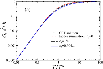
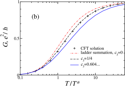
Figure 5: (Color online) (a) Conductance as a function of temperature for $K=1/2$. The results of ladder summation, (66) with $c_{3}=0$, are shown by dashed-dotted line ; the result of Eq. (66), with $c_{3}$ given by (52) is shown by solid line. The result available from CFT (multiplied by factor 2) is shown by pluses. Kane1992 ; Kane1992a ; Weiss1995 , together with our fit by (66) with $c_{3}=1/4$ shown as dashed line. (b) The same plot in log-linear scale.

Let us now illustrate the details of the behavior of $G(T)$ in the example of the well-known case $K=1/2$. Both high-temperature and low-temperature asymptotes of $G$ are interesting from the theoretical viewpoint, but one can expect the experimental variation of the conductance to be most visible at lower $T$, when $G\lesssim 1/2$. It is therefore useful to consider the variation of the conductance for fixed $K$ and different values of $c_{3}$. We take $K=1/2$ and and fix the low $T$ behavior in the form $G\simeq\tau^{2}$, with $\tau=T/T_{\ast}$ and $T_{\ast}\sim T_{0}|r|^{2}$. We then plot $G(\tau)$, obtained from (66) for several values of $c_{3}$ in Fig. 5, together with the exact solution, known from Kane1992 ; Kane1992a ; Weiss1995

$$G_{1/2}=1-\frac{1}{2\sqrt{3}\tau}\psi^{\prime}\left(\frac{1}{2}+\frac{1}{2\sqrt{3}\tau}\right)$$ (68)

where $\psi^{\prime}(x)$ the derivative of digamma function. For $K=1/2$, and the implied CFT value $c_{3}=1/4$ we can invert (66) and write

$$G=\frac{2\tau^{2}}{1+2\tau^{2}+\sqrt{1+8\tau^{2}}}$$ (69)

The Fig. 5 shows that the CFT solution lies between the curve corresponding to pure ladder summation, $c_{3}=0$, and the one with the above $c_{3}\simeq 0.60$. The proposed value $c_{3}=1/4$ fits the CFT solution rather precisely. This tells us that the approximation leading to (66) works rather well at the interaction strength $K=1/2$ ($g=3/5$) , provided the coefficient $c_{3}$ appropriate for the regularization scheme used in the CFT solution is taken. In fact, we show in the Appendix H, that the overall agreement criterion using the coefficient $C$, Eq. (67), is about 1 % in this case. For a further case reported ($K=1/3$ , $g=4/5$ ) Fendley1995 ; Fendley1995a the agreement is worse, about 10 %, which might be expected in this more strongly interacting situation.

Finally, we emphasize again that in any comparison with experiment the correct regularization scheme is determined by the details of the corresponding experimental setup. Indications of the possible inadequacy of the regularization scheme used in the CFT solutions exist. For instance, we tend to interpret the systematic deviation of the experimental data on the conductance between the quantum Hall edge states from the CFT prediction at low $T$ in Fendley1995a not as a shortcoming of the experiment, but rather as a consequence of choosing an inappropriate regularization. The correct regularization might lead to a different value of $c_{3}$ in (66), providing better agreement with experiment.

Appendix A From the Hamiltonian to the S-matrix

The continuum Hamiltonian (I.1) corresponds to a lattice model

$$H_{lat}=\sum_{i=-\infty}^{\infty}(c_{i}^{\dagger}c_{i+1}+h.c.)+\frac{1}{2}\sum_{j=1}^{2}(u_{1}+(-1)^{j}u_{2})c_{j}^{\dagger}c_{j},$$

at half-filling ($2k_{F}=\pi$) and with potential present at two adjacent sites.

In Eq. (I.1) we let $u_{1,2}(x)=u_{1,2}\delta_{a(1,2)}(x)$. Here $u_{1,2}$ are dimensionless quantities and $a_{1,2}$ is the range of the corresponding regularization of the $\delta$-function; at the end the limit $a_{1,2}\rightarrow 0$ will be taken.

Combining the two chiral fermions into a spinor quantity $\Psi^{\dagger}=(\psi_{R}^{\dagger},\psi_{L}^{\dagger})$ we can write the equation of motion as

$$i\partial_{t}\Psi = v_{F}\begin{pmatrix}i\partial_{x}+u_{1}(x)&u_{2}^{\ast}(x)\\ u_{2}(x)&-i\partial_{x}+u_{1}(x)\end{pmatrix}\Psi,$$

$$= v_{F}(i\sigma_{3}\partial_{x}+u_{1}(x)+u_{2}^{\prime}(x)\sigma_{1}+u_{2}^{\prime\prime}(x)\sigma_{2})\Psi,$$

with real and imaginary parts $u_{2}=u_{2}^{\prime}+iu_{2}^{\prime\prime}$. The formal solution of  (A) is

$$\Psi(x,t) = e^{i\omega t}\mathcal{T}(x,a)\Psi(a,0),$$ (71)

$$\mathcal{T}(x,a) = \mathcal{T}_{x}\exp i\int_{a}^{x}{dy}\,\sigma_{3}[v_{F}^{-1}\omega$$ (72)

$$+u_{1}(y)+u_{2}^{\prime}(y)\sigma_{1}+u_{2}^{\prime\prime}(y)\sigma_{2}],$$

where $\mathcal{T}_{x}$ stands for the $x$-ordering operator. In the long wavelength limit, $\omega\rightarrow 0$, we obtain

$$\mathcal{T}(x,a) = \exp[i\omega v_{F}^{-1}\sigma_{3}(x-a)],\quad x<0,$$

$$= \exp[i\omega v_{F}^{-1}\sigma_{3}x]\mathcal{T}_{0}\exp[-i\omega v_{F}^{-1}\sigma_{3}a],\quad x>0,$$

with $\mathcal{T}_{0}$ depending on $u_{1,2}(x)$. We assume first that the regularized $\delta$-functions in the definitons of $u_{1,2}(x)$ are identical, which means $a_{1}=a_{2}$. In this case

$$\mathcal{T}_{0}=\exp(iu_{1}\sigma_{3}-u_{2}^{\prime}\sigma_{2}+u_{2}^{\prime\prime}\sigma_{1})=\cosh b+\bm{b}\bm{\sigma}\frac{\sinh b}{b},$$ (74)

with ${\bm{b}}=(u_{2}^{\prime\prime},-u_{2}^{\prime},iu_{1})$ and $b^{2}=|u_{2}|^{2}-u_{1}^{2}$. This transfer matrix simplifies in two important cases : i) point-like impurity, when $u_{1}=|u_{2}|$ and ii) purely backward scattering impurity, $u_{1}=0$, $u_{2}\neq 0$. We have

$$\mathcal{T}_{0} = \begin{pmatrix}1+i|u_{2}|&iu_{2}^{\ast}\\ -iu_{2}&1-i|u_{2}|\end{pmatrix},\quad u_{1}=|u_{2}|,$$ (75)

$$\mathcal{T}_{0} = \begin{pmatrix}\cosh|u_{2}|&ie^{-i\phi}\sinh|u_{2}|\\ -ie^{i\phi}\sinh|u_{2}|&\cosh|u_{2}|\end{pmatrix},\quad u_{1}=0$$

with $e^{i\phi}=u_{2}/|u_{2}|$.

Let us also consider two further limiting cases, when the range of the forward scattering potential $u_{1}(x)$ is much longer (shorter) than the range of the backward scattering potential $u_{2}(x)$, i.e. $a_{1}\gg a_{2}$ ($a_{1}\ll a_{2}$ ). In these two cases we get

$$\mathcal{T}_{0}=\begin{pmatrix}e^{iu_{1}}\cosh|u_{2}|&ie^{-i\phi}\sinh|u_{2}|\\ -ie^{i\phi}\sinh|u_{2}|&e^{-iu_{1}}\cosh|u_{2}|\end{pmatrix}$$ (76)

for $a_{1}\gg a_{2}$ and

$$\mathcal{T}_{0}=\cos u_{1}\begin{pmatrix}\cosh|u_{2}|+i\tan u_{1}&ie^{-i\phi}\sinh|u_{2}|\\ -ie^{i\phi}\sinh|u_{2}|&\cosh|u_{2}|-i\tan u_{1}\end{pmatrix}$$ (77)

for $a_{1}\ll a_{2}$. By construction, the determinant of the transfer matrix is unity for arbitrary $u_{1,2}(x)$.

The elements of the scattering matrix for the incident waves $\sim e^{ikx}$ and $\sim e^{-ikx}$ at $x<0$ and $x>0$, respectively, are defined by the equation

$$\begin{pmatrix}t&\tilde{r}\\ 0&1\end{pmatrix}=\mathcal{T}_{0}.\begin{pmatrix}1&0\\ r&\tilde{t}\end{pmatrix}$$ (78)

Hence the scattering matrix is determined by the elements of the transfer-matrix $\mathcal{T}$ as

$$\mathcal{S}\equiv\begin{pmatrix}t&\tilde{r}\\ r&\tilde{t}\end{pmatrix}=\mathcal{T}_{22}^{-1}\begin{pmatrix}1&\mathcal{T}_{12}\\ -\mathcal{T}_{21}&1\end{pmatrix}$$

In the above two cases with $a_{1}=a_{2}$ we have

$$\mathcal{S} = \frac{1}{1-i|u_{2}|}\begin{pmatrix}1&iu_{2}^{\ast}\\ iu_{2}&1\end{pmatrix},\quad u_{1}=|u_{2}|,$$ (79)

$$\mathcal{S} = \begin{pmatrix}1/\cosh|u_{2}|&ie^{-i\phi}\tanh|u_{2}|\\ ie^{i\phi}\tanh|u_{2}|&1/\cosh|u_{2}|\end{pmatrix},\quad u_{1}=0.$$

Whereas for model potentials of different range we obtain

$$\mathcal{S}=e^{iu_{1}}\begin{pmatrix}1/\cosh|u_{2}|&ie^{-i\phi}\tanh|u_{2}|\\ ie^{i\phi}\tanh|u_{2}|&1/\cosh|u_{2}|\end{pmatrix}$$ (80)

for $a_{1}\gg a_{2}$ and

$$\mathcal{S}=\frac{1}{\cosh|u_{2}|-i\tan u_{1}}\begin{pmatrix}1/\cos u_{1}&ie^{-i\phi}\sinh|u_{2}|\\ ie^{i\phi}\sinh|u_{2}|&1/\cos u_{1}\end{pmatrix},$$ (81)

for $a_{1}\ll a_{2}$. We see that if the forward scattering $u_{1}$ has wider range, than $u_{2}$, then Eq. (80) differs from the second Eq. (79) only by the overall phase which is unimportant in physical observables. At the same time, if the model regularization of $u_{1}$ is narrower than $u_{2}$, the resulting Eq. (81) closely resembles the $S$-matrix in the double-barrier situation. Polyakov2003

Expanding the reflection coefficient in powers of $u_{1,2}$ and using (74), (80), (81) we have

$$|r| \simeq |u_{2}|-\frac{1}{3}|u_{2}|^{3},\quad a_{1}\gg a_{2},$$

$$|r| \simeq |u_{2}|-\frac{1}{6}|u_{2}|(u_{1}^{2}+2|u_{2}|^{2}),\quad a_{1}=a_{2},$$ (82)

$$|r| \simeq |u_{2}|-\frac{1}{6}|u_{2}|(3u_{1}^{2}+2|u_{2}|^{2}),\quad a_{1}\ll a_{2},$$

which shows that the forward scattering amplitude $u_{1}$ enters the reflection coefficient in the third order, i.e. beyond the Born approximation. Moreover the contribution of $u_{1}$ to the $S$-matrix depends also on the details of the microscopic Hamiltonian and the regularization of the model $\delta$-function potentials. This complication happens at the step (71); however, once the transfer matrix $\mathcal{T}_{0}$ in (A) is known, the connection to the scattering state basis is straightforward.

Returning to (2), (4), we notice that $\psi_{1}(x)$ obeys the equation of motion for right movers, and the spinor $\Psi_{R}^{\dagger}=(\psi_{1}^{+}(x),r\psi_{1}^{+}(-x))$ is an eigenstate (71) of (A) with the above property (78). We thus clarified the scattering states representation in the framework of the chiral Hamiltonian (1).

In the bosonization formulation, (5), the assumption is made that the forward scattering $u_{1}(x)$ can be completely removed from the Hamiltonian. This statement is not obvious, in general. Consider the redefinition $\varphi(x)=\tilde{\varphi}(x)-u_{1}sgn_{a1}(x)/2$, which eliminates the term with $u_{1}$ from Eq. (5), where the regularized sign function $sgn_{a1}(x)=-1+2\int_{-\infty}^{x}dy\,\delta_{a1}(y)$ is used. We have the backward scattering in the form

$$u_{2}(x)\cos(2\varphi(x)) = u_{2}(x)\cos(2\tilde{\varphi}(x)-u_{1}sgn_{a1}(x)),$$ (83)

$$\rightarrow u_{2}\,\delta(x)\cos(2\tilde{\varphi}(x)),$$

$$\rightarrow u_{2}\,\delta(x)\cos(2\tilde{\varphi}(x))\cos u_{1},$$

for the above cases of regularization with $a_{1}\gg a_{2}$ and $a_{1}\ll a_{2}$, respectively.

Appendix B Unitary transformation

We consider a transformation of the operators $J_{j}$

$$O_{j}(x)=U^{\dagger}J_{j}(x)U$$

with

$$U = \exp i\int_{-\infty}^{\infty}dx\,dy\,\theta(x-y)B_{j}(y)J_{j}(x),$$ (84)

$$= \exp i\int_{-\infty}^{\infty}dy\,B_{j}(y)\Theta_{j}(y),$$ (85)

$$\Phi_{j}(y) = \int_{y}^{\infty}dx\,J_{j}(x).$$ (86)

In our case we have $B_{j}(x)=B_{j}\delta(x)$ and we may denote the direction of $\mathbf{B}$ as ”1”, i.e. $\mathbf{B}\|\hat{e}_{1}$. Then we have the following set of equalities from the Kac-Moody relations (20)

$$[J_{1}(y),\Phi_{1}(x)] = \frac{i}{4\pi}\delta(x-y)$$

$${}[J_{1}(y),i\int_{-\infty}^{\infty}dx\,B_{1}(x)\Theta_{1}(x)] = -\frac{1}{4\pi}B_{1}(y)$$ (87)

$$J_{1}(y)U = U(J_{1}(y)-\frac{1}{4\pi}B_{1}(y))$$

And for $J^{+}(x)=J_{3}(x)+iJ_{2}(x)$ one has

$$[J^{+}(x),J_{1}(y)] = J^{+}(x)\delta(x-y)$$

$${}[J^{+}(x),\Theta_{1}(y)] = J^{+}(x)\theta(x-y)$$ (88)

$${}[J^{+}(x),i\int_{-\infty}^{\infty}dy\,B_{1}(y)\Theta_{1}(y)] = iJ^{+}(x)\int_{-\infty}^{x}dy\,B_{1}(y)$$

So that the relations between the operators are

$$O_{1}(x) = U^{\dagger}J_{1}(x)U=J_{1}(x)-\frac{1}{4\pi}B_{1}(x)$$ (89)

$$O_{3}(x)+iO_{2}(x) = U^{\dagger}J^{+}(x)U$$

$$= (J_{3}(x)+iJ_{2}(x))\exp i\int_{-\infty}^{x}dy\,B_{1}(y)$$

The transformation $U$ shifts the value of $O_{1}(x)$ by a $c-$number, so that strictly speaking, the operators $O_{j}(x)$ do not obey the same Kac-Moody algebra in the region where $B_{1}(x)\neq 0$. It is clear, though that this might affect only the physically non-observable component of the fermionic density and is therefore not important.

Appendix C Equations of motion in current operator formalism

In this section we focus on the time evolution of the observables $J_{3}(-x)$, $\widetilde{J}_{3}(x)$, Eqs. (22), (23), using the relation $i\partial_{t}A=[A,H]$. It is more convenient to use the representation (27), with $O(x)=J_{3}(x)\Theta(-x)+\widetilde{J}_{3}(x)\Theta(x)$. In terms of operators $O_{j}(x)$ one has

$$\rho_{s}(x) = (O_{3}(x)-O_{3}(-x))$$ (91)

$$j_{s}(x) = v_{F}(O_{3}(x)+O_{3}(-x))$$

Using (20) and formulas of Appendix B, it can be easily shown that we have $-\partial_{t}O_{3}(x)=\partial_{x}O_{3}(x)$ in the leads, $|x|>L$, whereas in the interacting region $a<|x|<L$ we obtain

$$-\partial_{t}O_{3}(x)=\partial_{x}O_{3}(x)-g\partial_{x}O_{3}(-x),$$ (92)

where we let $v_{F}=1$. Since $O_{3}(x)$ is the observable density, the relation (92) looks deceptively close to the desired answer. However, in the region of the barrier $|x|<a$ (with $\mathbf{B}\|O_{1}$) we have

$$-\partial_{t}O_{3}(x)=\partial_{x}O_{3}(x)+B(x)O_{2}(x),$$

and the $O_{2}$ component comes into play. (In other words, for the partially reflecting barrier, the observable of our problem, $\widetilde{J}_{3}(x)$, includes the eigenmode operator $J_{2}(x)$.) Therefore it is necessary to consider also the time evolution of operator $O_{2}$, which reads

$$-\partial_{t}O_{2}(x)=\partial_{x}O_{2}(x)-4\pi gO_{1}(x)O_{3}(-x),$$ (93)

at $a<|x|<L$ and $-\partial_{t}O_{2}(x)=\partial_{x}O_{2}(x)+B(x)O_{3}(x)$, at $|x|<a$. The four-fermion object $O_{1}(x)O_{3}(-x)$ is not reduced to $O_{2}(-x)$ and therefore we do not obtain a closure of the equations of motion.

Our situation is somewhat similar to the well-known Heisenberg model of spins with pairwise exchange interaction. Due to the non-commutative character of spin operators, the attempt to write the exact time evolution of spin leads to an infinite series of coupled equations, including ever increasing numbers of spins. The approximate solutions are obtained by truncating this series at some step, according to a certain criterion, and discarding higher terms as inessential. Izyumov1988 In magnetism, these criteria might be (i) low temperatures in the magnetically ordered phase, $T\ll T_{c}$, (ii) large value of spin $S$ or (iii) wide range of interaction. In our case, we choose the criterion of relevancy of operators, i.e. their importance in the logarithmically divergent theory.

We now briefly discuss the dynamics of $O_{4}(x)\equiv 4\pi O_{1}(x)O_{3}(-x)$. The compound operator $O_{4}(x)$ consists of four fermion operators and may be decomposed into the normally ordered part and a part, representing internal contractions. To clarify the notation we write $\psi_{1}(x)=a_{\uparrow}(x)$, $\psi_{2}(-x)=a_{\downarrow}(x)$, then we have

$$O_{4}(x) = \pi(a_{\uparrow}^{\dagger}(x)a_{\downarrow}(x)+a_{\downarrow}^{\dagger}(x)a_{\uparrow}(x))$$ (94)

$$\times(a_{\uparrow}^{\dagger}(-x)a_{\uparrow}(-x)-a_{\downarrow}^{\dagger}(-x)a_{\downarrow}(-x))$$

Contracting here, we get $O_{4}(x)-\!:\!O_{4}(x)\!\!:=-x^{-1}O_{2}(\bar{x})$ with (cf. Eq. (29))

$$O_{2}(\bar{x})=\frac{1}{4i}(a_{\uparrow}^{\dagger}(x)a_{\downarrow}(-x)+a_{\uparrow}^{\dagger}(-x)a_{\downarrow}(x))+h.c.$$ (95)

which does not coincide with $O_{2}(x)=(2i)^{-1}a_{\uparrow}^{\dagger}(x)a_{\downarrow}(x)+h.c.$ We may write

$$O_{2}(\bar{x})\simeq O_{2}(-x)-x\partial_{x}O_{2}(-x)+\ldots$$ (96)

and, dropping the less relevant higher derivatives, obtain from (93)

$$-\partial_{t}O_{2}(x)\simeq\partial_{x}O_{2}(x)+g(x^{-1}-\partial_{x})O_{2}(-x)-g:\!O_{4}(x)\!:$$

which means that the most relevant part of the operator $O_{4}(x)$ has the form

$$O_{4}(x)\simeq(-1/x+\partial_{x})O_{2}(-x).$$ (97)

Regarding the normally ordered part $:O_{4}(x):$, its time evolution is given by

$$-\partial_{t}:\!O_{4}(x)\!: = 4\pi:\!O_{3}(-x)\partial_{x}O_{1}(x)-O_{1}(x)\partial_{x}O_{3}(-x)\!:$$

$$+4\pi g:\!O_{5}(x)\!:$$

$$O_{5}(x) = 4\pi O_{1}(x)O_{3}^{2}(-x)+O_{1}(x)\partial_{x}O_{3}(x)$$

i.e. described by new operators, not reduced to simple spatial derivatives of $:O_{4}(x):$. Such derivative objects (i) obey an infinite set of coupled equations and (ii) possess formal scaling dimension greater than two, and hence are irrelevant in the RG sense.

Our strategy of such truncation (97) is successful only in part, as we explain in the next Appendix D.

Appendix D Solution of the equation of motion

Taking a Fourier transform in time $t$, and introducing the vector

$$\Psi(x,\omega)=\left[O_{3}(x,\omega),O_{3}(-x,\omega),O_{2}(x,\omega),O_{2}(-x,\omega)\right]$$

the above truncated set of equations can be written as

$$\partial_{x}\Psi(x,\omega) =\hat{D}_{0}(\omega,x)|_{g=0}\Psi(x,\omega),\quad|x|>L$$ (98)

$$\hat{D}_{1}\partial_{x}\Psi(x,\omega) =\hat{D}_{0}(\omega,x)\Psi(x,\omega),\quad a<|x|<L$$

with

$$\hat{D}_{0}(\omega,x) = \begin{pmatrix}i\omega,&0,&0,&0\\ 0,&-i\omega,&0,&0\\ 0,&0,&i\omega,&-gf(x)\\ 0,&0,&-gf(x),&-i\omega\end{pmatrix}$$ (99)

$$\hat{D}_{1} = \begin{pmatrix}1,&-g,&0,&0\\ -g,&1,&0,&0\\ 0,&0,&1,&-g\\ 0,&0,&-g,&1\end{pmatrix}$$ (100)

and the fermionic correlation function at finite temperature

$$f(x)=\frac{2\pi T}{\sinh 2\pi Tx}$$ (101)

The solution to (98) is given by the $x-$ordered exponent

$$\Psi(x,\omega) = \hat{U}(x,y)\Psi(y,\omega)$$ (102)

$$\hat{U}(x,y) = T_{x}\exp\int_{y}^{x}dz\,\hat{D}_{1}^{-1}\hat{D}_{0}(\omega,z),$$ (103)

similarly to (71), but now with transfer-matrix $\hat{U}(x,y)$ for densities. The transfer-matrix in the region of the barrier $|x|<a$ is already known and given by

$$\hat{U}(a,-a)=\begin{pmatrix}\cos 2\theta,&0,&\sin 2\theta,&0\\ 0,&\cos 2\theta,&0,&-\sin 2\theta\\ -\sin 2\theta,&0,&\cos 2\theta,&0\\ 0,&\sin 2\theta,&0,&\cos 2\theta\end{pmatrix}$$ (104)

The overall transfer-matrix over the interaction region is

$$\hat{U}(L,-L)=\hat{U}(L,a).\hat{U}(a,-a).\hat{U}(-a,-L)$$ (105)

Finally we observe that the definition of $\Psi(x)$ implies that the transfer matrix connecting opposite points should satisfy the boundary condition:

$$\hat{U}(x,-x)\Psi(-x,\omega)=\hat{I}.\Psi(-x,\omega)$$ (106)

$$\hat{I}=\begin{pmatrix}0,&1,&0,&0\\ 1,&0,&0,&0\\ 0,&0,&0,&1\\ 0,&0,&1,&0\end{pmatrix}$$ (107)

and we should choose a solution, by demanding that the scattered component, $O_{2}$, is absent in the incoming wave, i.e. $\Psi_{3}(-\infty,\omega)=0$.

We consider here only the technically feasible limit, $\omega=0$. In this case $\hat{U}(x,L)=\hat{U}(-L,-x)=1$ in the leads, $x>L$. In the interacting region

$$\hat{U}(L,a) = \begin{pmatrix}1,&0,&0,&0\\ 0,&1,&0,&0\\ 0,&0,&e^{-g^{2}\Lambda}\cosh g\Lambda,&-e^{-g^{2}\Lambda}\sinh g\Lambda\\ 0,&0,&-e^{-g^{2}\Lambda}\sinh g\Lambda,&e^{-g^{2}\Lambda}\cosh g\Lambda\end{pmatrix}$$ (108)

$$\Lambda = (1-g^{2})^{-1}\int_{a}^{L}dx\,f(x)=(1-g^{2})^{-1}\ln\left(\frac{\tanh\pi TL}{\tanh\pi Ta}\right)$$ (109)

A similar contribution on the negative semiaxis, $\hat{U}(-a,-L)$, is obtained from (108) by the change $\Lambda\to-\Lambda$. Overall we have

$$\hat{U}(\infty,-\infty)=\begin{pmatrix}\cos 2\theta,&0,&-e^{g^{2}\Lambda}\sin 2\theta\cosh g\Lambda,&-e^{g^{2}\Lambda}\sin 2\theta\sinh g\Lambda\\ 0,&\cos 2\theta,&e^{g^{2}\Lambda}\sin 2\theta\sinh g\Lambda,&e^{g^{2}\Lambda}\sin 2\theta\cosh g\Lambda\\ e^{-g^{2}\Lambda}\sin 2\theta\cosh g\Lambda,&e^{-g^{2}\Lambda}\sin 2\theta\sinh g\Lambda,&\cos 2\theta,&0\\ -e^{-g^{2}\Lambda}\sin 2\theta\sinh g\Lambda,&-e^{-g^{2}\Lambda}\sin 2\theta\cosh g\Lambda,&0,&\cos 2\theta\end{pmatrix}$$

Solving Eq. (106) together with the above condition $\Psi_{3}(-\infty)=0$, we find

$$\Psi(-\infty)=(\cos^{2}\theta+e^{2g\Lambda}\sin^{2}\theta,\cos^{2}\theta-e^{2g\Lambda}\sin^{2}\theta,0,-e^{g(1-g)\Lambda}\sin 2\theta)$$ (110)

which is the desired solution. Let us briefly discuss it.

We observe that the d.c. current $j(x)=O_{3}(x)+O_{3}(-x)$ is independent of $x$, as it should be. This property follows from the form of matrix (108) and condition (106). The relation of the current to the voltage bias defines the conductance of the system. In our definitions, the voltage bias is proportional to the difference in number of incoming left- and right-going electrons, which is $2O_{3}(-\infty)=2\Psi_{1}(-\infty)$, so that the conductance is

$$G = \frac{j(x)}{2O_{3}(-\infty)}=\frac{1}{2}\left(\frac{O_{3}(\infty)}{O_{3}(-\infty)}+1\right)$$ (111)

$$= \frac{\cos^{2}\theta}{\cos^{2}\theta+e^{2g\Lambda}\sin^{2}\theta}$$

which coincides with the above result (11).

At first glance, the result (110) should thus be viewed as satisfactory. However there are details, involved in its derivation, which spoil the significance of this approach. First we notice that, by keeping less relevant gradient term in the above relation, (97), we get the appearance of $g^{2}$ terms in the definition of $\Lambda$, eq. (109), and also in the exponents, $e^{g^{2}\Lambda}$, in (108) – (110). Further, trying a different approximation instead of (97), e.g. $O_{4}(x)\simeq(-1/x+\partial_{x})O_{2}(x)$, would not produce the above renormalized value of conductance.

Therefore we conclude that using the equations of motion method and persisting with the current operator algebra leads to ambiguities, connected with the non-local character of the interaction.

Appendix E Calculation of corrections: zero temperature

Proceeding as described in Sec. V.1, we find corrections to the conductance, or to $Y$ in (31). In the first order of $g$ the correction from the diagrams of the type $\{4\}$ has the form

$$\delta Y^{\{4\}}=-g(1-Y^{2})\int_{a}^{L}\frac{dx}{x}=-g(1-Y^{2})\Lambda_{0}$$ (112)

In the second order of $g$ we have two sets of diagrams for corrections to the conductance. The diagrams containing two fermionic loops lead to the following expression :

$$\delta Y^{\{4,2\}} = g^{2}Y(1-Y^{2})\int_{a}^{L}\frac{dx_{1}dx_{2}}{2(x_{1}+x_{2})^{2}}$$ (113)

$$= \frac{1}{2}g^{2}Y(1-Y^{2})(\Lambda_{0}-2\ln 2)$$

where $x_{1,2}$ are two points of fermionic interaction.

All diagrams consisting of only one loop, $\{6\}$ in above notation, produce the correction

$$\delta Y^{\{6\}}=-g^{2}Y(1-Y^{2})\int_{a}^{L}\frac{dx_{1}dx_{2}}{x_{1}x_{2}}=-g^{2}Y(1-Y^{2})\Lambda_{0}^{2}$$ (114)

We should mention that individual diagrams in the set $\{6\}$ (and higher orders) may contain singularities of the form $(x_{1}-x_{2})^{-1}$ etc. However these singularities cancel each other in the resulting expressions. For example, one finds two particular contributions $x_{1}^{-1}(x_{1}-x_{2})^{-1}$ and $x_{2}^{-1}(x_{2}-x_{1})^{-1}$ whose sum leads to the above “regular” form, $(x_{1}x_{2})^{-1}$, in (114).

In the third order, we have to analyze the following types of the diagrams : $\{4,2,2\}$, $\{4,4\}$, $\{6,2\}$, $\{8\}$. We assume the ordered sequence, $L>x_{1}>x_{2}>x_{3}>a$, in all integrals below. Performing rather long computer calculations (the stable routine in Mathematica requires about ten hours of computation time for dual-core 3 GHz processor), we obtain

$$\delta Y^{\{4,2,2\}} = -g^{3}(1-Y^{2})\int{\prod dx_{i}}$$ (115)

$$\times \left[\frac{3Y^{2}}{(x_{1}+x_{2}+x_{3})^{3}}+\frac{1}{(x_{1}+x_{2}-x_{3})^{3}}\right]$$

$$= -g^{3}(1-Y^{2})(1+Y^{2})\frac{\Lambda_{0}}{4},$$

$$\delta Y^{\{4,4\}} = -g^{3}(1-Y^{2})^{2}\int{\prod dx_{i}}$$ (116)

$$\times \left[\frac{1}{x_{1}(x_{2}+x_{3})(x_{1}+x_{2}+x_{3})}+(\mbox{symm.})\right]$$

$$= -g^{3}(1-Y^{2})^{2}\frac{1}{4}(\Lambda_{0}^{2}+2\Lambda_{0}(1-\ln 2)),$$

$$\delta Y^{\{6,2\}} = 2g^{3}(1-Y^{2})Y^{2}\int{\prod dx_{i}}$$ (117)

$$\times \left[\frac{1}{x_{1}(x_{2}+x_{3})^{2}}+(\mbox{symm.})\right]$$

$$= g^{3}(1-Y^{2})Y^{2}\Lambda_{0}(\Lambda_{0}-2\ln 2),$$

$$\delta Y^{\{8\}} = 2g^{3}(1-Y^{2})\int{\prod dx_{i}}\left[\frac{1-3Y^{2}}{x_{1}x_{2}x_{3}}\right.$$

$$+ \left.\frac{1-Y^{2}}{(x_{1}+x_{2})(x_{2}+x_{3})(x_{3}+x_{1})}\right]$$

$$= g^{3}(1-Y^{2})\left[\frac{1-3Y^{2}}{3}\Lambda_{0}^{3}+(1-Y^{2})\frac{\pi^{2}}{12}\Lambda_{0}\right].$$

In the final expressions (115), (116), (E) we omitted finite parts, $O(\Lambda^{0})$, which are unimportant in the order $g^{3}$. These expressions lead to Eq. (43) above.

Appendix F Calculation of corrections: finite temperature

In case of finite temperature we proceed in the same way as for $T=0$ , only with the integration replaced by a summation over Matsubara frequencies. Introducing the scaling variable $\Lambda$ according to (47) we have for $a\ll\xi=v_{F}/\pi T\ll L$

$$\delta Y^{\{4\}} = -g(1-Y^{2})\Lambda,$$

$$\delta Y^{\{4,2\}} = g^{2}Y(1-Y^{2})\int_{a/\xi}\frac{2d\bar{x}_{1}d\bar{x}_{2}}{\sinh^{2}2(\bar{x}_{1}+\bar{x}_{2})}$$

$$= \frac{1}{2}g^{2}Y(1-Y^{2})(\Lambda-3\ln 2),$$

where $x_{1,2}$ are two points of fermionic interaction, and $\bar{x}_{i}=x_{i}/\xi$. In the last equality in the right-hand side of Eq. (F), we shall neglect the terms $\sim O(1)$.

Instead of $\Lambda_{0}^{2}$ in the expression (114) for $\delta Y^{\{6\}}$ we now have the following integral

$$\int_{a/\xi}^{L/\xi}{d\bar{x}_{1}d\bar{x}_{2}}\frac{3\cosh(\bar{x}_{1}+\bar{x}_{2})+\cosh(\bar{x}_{1}-\bar{x}_{2})}{\sinh(2\bar{x}_{1})\sinh(2\bar{x}_{2})\cosh(\bar{x}_{1}+\bar{x}_{2})}$$

$$= \int_{\tau_{0}}^{\tau_{L}}\frac{d\tau_{1}d\tau_{2}}{\tau_{1}\tau_{2}}\left(1-\frac{1}{2}\frac{\tau_{1}\tau_{2}}{1+\tau_{1}\tau_{2}}\right)$$

$$= \Lambda^{2}-F[\tau_{L},\tau_{0}]$$

$$\rightarrow \Lambda^{2}-\frac{\pi^{2}}{24},\quad T\gg v_{F}/L$$

with $\tau_{i}=\tanh\bar{x}_{i}$ . The integration limits in (F) are $\tau_{0}=\tanh(a/\xi)$ and $\tau_{L}=\tanh(L/\xi)$. Here $F[\tau_{L},\tau_{0}]=L_{2}(-\tau_{0}\tau_{L})-(L_{2}(-\tau_{L}^{2})+L_{2}(-\tau_{0}^{2}))/2$ and $L_{2}(x)=\sum_{1}^{\infty}x^{n}/n^{2}$ is the dilogarithm function. We have $F[\tau_{L},\tau_{0}]=0$ in the limit $T\ll v_{F}/L$.

In contrast to the $T=0$ case, the expressions now become extremely cumbersome in the third order of $g$. The summation over Matsubara frequencies lead to expressions involving sums and products of exponents $\exp(\bar{x}_{i})$. A general criterion for the correctness of intermediate expressions is the property a change of sign of each individual diagram upon performing the reflection transformation $z_{i}\rightarrow-z_{i}$.

An additional check of the validity of calculation is the observation that we should get zero correction to $G=1$ in the absence of the barrier, $\theta=0$, and to $G=0$ for the fully reflecting barrier, $\theta=\pi/2$, for arbitrary $T$. This is not a trivial statement, because each diagram in third order contains a prefactor, either $\cos 8\theta$, or $\cos 4\theta$ or $\cos 0\theta=1$. We verified that the algebraic expressions canceled each other in this case.

The actual expressions are not shown here, and we describe our method of analysis below.

Let us consider an expression of the form of a triple integral, relevant to our discussion in Sec. V

$$f(a)=\int_{a}^{L}dz_{1}\int_{z_{1}}^{L}dz_{2}\int_{z_{2}}^{L}dz_{3}\bar{f}[z_{1},z_{2},z_{3}].$$ (121)

We assume that $f(a)\simeq-c\ln a+\ldots$ at $a\rightarrow 0$ and wish to determine the coefficient $c$ in this asymptotic behavior. We have

$$c=-\lim_{a\rightarrow 0}\frac{df(a)}{d\ln a}=\lim_{a\rightarrow 0}\int_{a}^{L}dz_{2}\int_{z_{2}}^{L}dz_{3}\,a\bar{f}[a,z_{2},z_{3}]$$ (122)

Here taking the limit in the integrand may lead to incorrect results. We have two possibilities for the behavior of the quantity $\bar{f}_{2}[a,z_{2}]=\int_{z_{2}}^{L}dz_{3}\,a\bar{f}[a,z_{2},z_{3}]$, for small $a$, namely $\bar{f}_{2}[a\rightarrow 0,z_{2}]\sim a/(z_{2}+a)^{2}$ and $\bar{f}_{2}[a\rightarrow 0,z_{2}]\sim 1$. The first type of contribution, $\bar{f}_{2}\sim a/(z_{2}+a)^{2}$, is always important and survives in the limit of $T\rightarrow 0$. Recalling that $\bar{f}[a,z_{2},z_{3}]$ is exponentially suppressed at $z_{i}\gtrsim\xi$, we see that the case $\bar{f}_{2}[a,z_{2}]\sim 1$ contributes to $c$ only at finite temperatures, $L\gg\xi$ ; typically, we find $\bar{f}_{2}[a\rightarrow 0,z_{2}]\sim(\xi\cosh(2z_{2}/\xi))^{-1}$.

Therefore the recipe for the determination of $c$ is first to determine the limiting form of $\bar{f}_{2}$, taking $z_{2}\sim a\ll\xi$ ; in this case the expressions are drastically simplified. This will determine $c$ at $T\rightarrow 0$. To this term we should add the contribution $\lim_{a\rightarrow 0}a\bar{f}[a,z_{2},z_{3}]$, integrated over $z_{2}$ in the interval $(0,\infty)$ ; the sum of these two contributions gives the value of $c$ at finite temperatures, $L\gg\xi$.

Appendix G ”Non-universality of higher terms” in $\beta-$function

In a very general sense the $\beta$-function of the RG-equation is non-universal: it depends on the precise definition of the scaling quantity $g$ . Let the RG equation read

$$dg_{r}/d\Lambda=\beta(g_{r})=b_{2}g_{r}^{2}+b_{3}g_{r}^{3}+b_{4}g_{r}^{4}+\ldots$$ (123)

and consider a change of variable $g_{r}=\bar{g}+c_{2}\bar{g}^{2}+c_{3}\bar{g}^{3}$. With the same accuracy we have

$${d\bar{g}}/{d\Lambda} = \beta(\bar{g})=\beta(g)/(dg/d\bar{g})=b_{2}\bar{g}^{2}+b_{3}\bar{g}^{3}$$ (124)

$$+(b_{4}+b_{3}c_{2}+b_{2}(c_{2}^{2}-c_{3}))\bar{g}^{4}+\ldots$$

which shows that only the two first two coefficients $b_{2}$ and $b_{3}$ are invariant. Since $b_{4}$ is associated with the three-loop contribution, one may speak about a non-universality of the$\ \beta$-function beyond two-loop order.

Let us elucidate the origin of the Eq. (124), and compare it with the equation obtained in the Callan-Symanzik approach. In the Gell-Mann–Low approach we perform our calculations with the running coupling constant $g_{r}$ and add counterterms to the Hamiltonian in order to achieve the finite value of the bare constant $g_{0}$. One can show that the above value of $dg_{r}/d\Lambda=-(\partial g_{0}/\partial\Lambda)/(\partial g_{0}/\partial g_{r})$ is obtained from the expression

$$g_{0} = g_{r}-b_{2}\Lambda g_{r}^{2}-(b_{3}\Lambda-b_{2}^{2}\Lambda^{2})g_{r}^{3}$$ (125)

$$-(b_{4}\Lambda-\frac{5}{2}b_{2}b_{3}\Lambda^{2}+b_{2}^{3}\Lambda^{3})g_{r}^{4}+\ldots$$

If we make the above change $g_{r}\rightarrow\bar{g}$ in the right-hand side of (125) and use the same recipe for $d\bar{g}/d\Lambda$, we return to (124).

In the CS approach we fix the bare value $g_{0}$ and calculate the renormalized quantity $g_{r}(g_{0},\Lambda)$. Inverting the equation $g_{0}(g_{r},\Lambda)$ and using the same recipe we find $dg_{r}/d\Lambda$. One can check that

$$g_{r} = g_{0}+b_{2}\Lambda g_{0}^{2}+(b_{3}\Lambda+b_{2}^{2}\Lambda^{2})g_{0}^{3}$$ (126)

$$+(b_{4}\Lambda+\frac{5}{2}b_{2}b_{3}\Lambda^{2}+b_{2}^{3}\Lambda^{3})g_{0}^{4}+\ldots$$

Assume now that we have changed the starting value $g_{0}=\bar{g}_{0}+c_{2}\bar{g}_{0}^{2}+c_{3}\bar{g}_{0}^{3}+\ldots$, according to above prescription. Evidently, the expansion for $g_{r}(\bar{g}_{0},\Lambda)$ will be different from (126), as well as the inverse function $\bar{g}_{0}(g_{r},\Lambda)$ will not coincide with (125). One can verify however that the $\beta$-function, $-(\partial\bar{g}_{0}/\partial\Lambda)/(\partial\bar{g}_{0}/\partial g_{r})$, is given by the same Eq. (123) and not by Eq. (124). This fact becomes rather obvious, when we notice that only the left-hand side of (125) is changed and it corresponds to a change in the boundary condition for $g_{r}(\Lambda)$ rather than to a change in the differential equation for it.

Appendix H Comparison to CFT solution

Consider the differential equation

$$[-\partial_{y}^{2}+se^{Ky}+e^{y}]\Psi(y)=0$$ (127)

such that $\Psi(y\rightarrow\infty)=0$ and $\Psi(y\rightarrow-\infty)=y-y_{0}$. Here

$$s=K^{2}\exp(2(1-K)\Lambda)$$

and $\Lambda=\ln(T_{0}/T)$. For given $s$ one finds a solution $\Psi(y)$ characterized by a unique value $y_{0}$. Then, according to Lukyanov, Lukyanov2007 the conductance can be determined as

$$G(T)=1+Ks\frac{\partial y_{0}}{\partial s}=1+\frac{K}{2(1-K)}\frac{\partial y_{0}}{\partial\Lambda}$$ (128)

We now fix the overall temperature scale $\tau=T/T_{0}$ by the high-$T$ behavior, $G\simeq 1-\tau^{2(K-1)}$, and ask what is the coefficient $C$ in the asymptotic low temperature expression $G\simeq C\tau^{2(K^{-1}-1)}$. To answer this question, we slightly rewrite the differential equation. Introducing a new variable $z=2e^{y/2}$ we have

$$[-\partial_{z}^{2}-z^{-1}\partial_{z}+1+s(z/2)^{2(K-1)}]\Psi(z)=0$$ (129)

At $s=0$ (i.e. $T\rightarrow\infty$) the solution is a modified Bessel function $\Psi(z)=-2K_{0}(z)$. At infinitesimal $s$ we seek a solution in perturbation theory as $\Psi(z)=-2K_{0}(z)+sR(z)+O(s^{2})$. After some calculation we find the conductance $G(T)\simeq 1-Ks\mathcal{F}(K)$ with $\mathcal{F}(K)\equiv R(0)$ given by

$$\mathcal{F}(K) = \Gamma^{2}[K]\int_{0}^{\infty}{}_{2}F_{1}(K,K,1;-\kappa)\frac{d\kappa}{1+\kappa}$$ (130)

$$= {\Gamma^{4}[K]}/{\Gamma[2K]}\;.$$

In the opposite limit, $s\rightarrow\infty$ ($T=0$), we choose a variable $z=(2\sqrt{s}/K)e^{Ky/2}$ and arrive at an equation

$$[-\partial_{z}^{2}-z^{-1}\partial_{z}+1+s_{1}(z/2)^{2(K^{-1}-1)}]\Psi(z)=0,$$ (131)

with $s_{1}=s^{-1/K}K^{2(K^{-1}-1)}\ll 1$. The solution is found similarly to (129) and we get $G(T)\simeq-s\partial_{s}s_{1}\mathcal{F}(K^{-1})$. Comparing the two solutions we obtain the prefactor

$$C=\left(K^{3}\mathcal{F}(K)\right)^{1/K}K^{-3}\mathcal{F}(K^{-1})$$ (132)

In the particular case of $K=1/2$ we have $C=\pi^{4}/48=2.029\ldots$, in accordance with Ref. [Weiss1995, ]. For $K=1/3$ we get $C=10.064558\ldots$, a value slightly different from $C=10.0638$ reported in Fendley1995 ; Fendley1995a , where it was obtained by numerical solution of an integral equation. If we take $c_{3}=1/4$ in (67), then we would obtain $C=2$ ($C=9$) for the cases of $K=1/2$ ($K=1/3$), in good agreement with the above CFT values. It should be noted, however, that apart from this agreement in the matching coefficient $C$, the theory in Lukyanov2007 provides the value of unity for $G$ in the clean wire, whereas the previous works Weiss1995 ; Fendley1995 ; Fendley1995a gave $G=K$ in that case.

References

- (1) A. O. Gogolin, A. A. Nersesyan, and A. M. Tsvelik, Bosonization and Strongly Correlated Systems (Cambridge University Press, Cambridge, 1998).
- (2) T. Giamarchi, Quantum Physics in One Dimension (Clarendon Press, Oxford, 2003).
- (3) W. Apel and T. M. Rice, Phys. Rev. B 26, 7063 (1982).
- (4) C. L. Kane and M. P. A. Fisher, Phys. Rev. B 46, 15233 (1992).
- (5) C. L. Kane and M. P. A. Fisher, Phys. Rev. Lett. 68, 1220 (1992).
- (6) D. L. Maslov and M. Stone, Phys. Rev. B 52, R5539 (1995).
- (7) I. Safi and H. J. Schulz, Phys. Rev. B 52, R17040 (1995).
- (8) Y. Oreg and A. M. Finkel’stein, Phys. Rev. B 54, R14265 (1996).
- (9) A. Furusaki and N. Nagaosa, Phys. Rev. B 47, 4631 (1993).
- (10) U. Weiss, R. Egger, and M. Sassetti, Phys. Rev. B 52, 16707 (1995).
- (11) P. Fendley, A. W. W. Ludwig, and H. Saleur, Phys. Rev. B 52, 8934 (1995).
- (12) P. Fendley, A. W. W. Ludwig, and H. Saleur, Phys. Rev. Lett. 74, 3005 (1995).
- (13) D. Yue, L. I. Glazman, and K. A. Matveev, Phys. Rev. B 49, 1966 (1994).
- (14) D. G. Polyakov and I. V. Gornyi, Phys. Rev. B 68, 035421 (2003).
- (15) T. Enss, V. Meden, S. Andergassen, X. Barnabé-Thériault, W. Metzner, and K. Schönhammer, Phys. Rev. B 71, 155401 (2005).
- (16) S. Andergassen, T. Enss, V. Meden, W. Metzner, U. Schollwöck, and K. Schönhammer, Phys. Rev. B 73, 045125 (2006).
- (17) Y. Oreg and A. M. Finkel’stein, Phys. Rev. Lett. 74, 3668 (1995).
- (18) U. Weiss, Sol. State Comm. 100, 281 (1996).
- (19) C. G. Callan, I. R. Klebanov, A. W. W. Ludwig, and J. M. Maldacena, Nucl. Phys. B 422, 417 (1994).
- (20) I. Affleck and A. W. W. Ludwig, Nucl. Phys. B 360, 641 (1991).
- (21) M. Fabrizio and A. O. Gogolin, Phys. Rev. B 51, 17827 (1995).
- (22) Y. Izyumov and Y. Skryabin, Statistical mechanics of magnetically ordered systems (Consultants Bureau, New York, 1988).
- (23) I. Suslov, J. Exp.Theor. Phys. 100, 1188 (2005).
- (24) P. Ramond, Field Theory: a Modern Primer (Addison-Wesley, Reading, 1989).
- (25) K. Higashijima and K. Nishijima, Progr. Theor. Phys. 64, 2179 (1980).
- (26) A. W. W. Ludwig and K. J. Wiese, Nucl. Phys. B 661, 577 (2003).
- (27) D. N. Aristov and P. Wölfle, Europhysics Letters 82, 27001 (2008).
- (28) S. L. Lukyanov and P. Werner, J. Stat. Mech.: Theory and Experiment 2007, P06002 (2007).