On the average number of rational points
on curves of genus 2

1. Introduction

For $N>0$, let ${\mathcal{C}}_{N}$ denote the set of all genus $2$ curves

$$C:y^{2}=F(x,z)=f_{6}\,x^{6}+f_{5}\,x^{5}z+\dots+f_{1}\,xz^{5}+f_{0}\,z^{6}$$

with integral coefficients $f_{j}$ such that $|f_{j}|\leq N$ for all $j$. ($C$ is considered in the weighted projective plane with weights $1$ for $x$ and $z$ and weight $3$ for $y$.)

In this note, we sketch heuristic arguments that lead to the following conjectures.

Conjecture 1.

There is a constant $\gamma>0$ such that

$$\frac{\sum_{C\in{\mathcal{C}}_{N}}\#C({\mathbb{Q}})}{\#{\mathcal{C}}_{N}}\sim\frac{\gamma}{\sqrt{N}}\,.$$

In particular, the density of genus $2$ curves with a rational point is zero.

The second part of this conjecture is analogous to Conjecture 2.2 (i) in [PV], which considers hypersurfaces in ${\mathbb{P}}^{n}$.

If $C$ is a curve of genus 2 as above and $P=(a:y:b)$ is a rational point on $C$ (i.e., we have $F(a,b)=y^{2}$ with $a,b$ coprime integers), then we denote by $H(P)$ the height $H(a:b)=\max\{|a|,|b|\}$ of its $x$-coordinate.

Conjecture 2.

Let $\varepsilon>0$. Then there is a constant $B_{\varepsilon}$ and a Zariski open subset $U_{\varepsilon}$ of the ‘coefficient space’ ${\mathbb{A}}^{7}$ such that for all $C\in{\mathcal{C}}_{N}\cap U_{\varepsilon}$ and all rational points $P$ on $C$, we have

$$H(P)\leq B_{\varepsilon}N^{13/2+\varepsilon}\,.$$

The reason for restricting to $U_{\varepsilon}$ is that one should expect infinite families of curves with larger points (at least over sufficiently large number fields). In general, we still expect the following to hold.

Conjecture 3.

There are constants $\kappa$ and $B$ such that every rational point $P$ on any curve $C\in{\mathcal{C}}_{N}$ satisfies $H(P)\leq BN^{\kappa}$.

If we restrict to quadratic twists of a fixed curve, then the ABC Conjecture implies such a bound with $\kappa=1/2$, see [Gra].

Note that Conjecture 3 says in particular that the height of a point on $C$ is polynomially bounded by the height of $C$. If a statement like the above could be proved for some explicit $\kappa$ and $B$, then this would immediately imply that there is a polynomial time algorithm that determines the set of rational points on a given curve $C$ of genus 2. More precisely, it would be polynomial time in $N$ (and not in the input length, which is roughly $\log N$). If we assume that the Mordell-Weil group of the Jacobian $J$ of $C$ is known, then we obtain a very efficient algorithm, since we only have to check all points in $J({\mathbb{Q}})$ of logarithmic height $\ll\log N$.

Similar statements can be formulated for other families of curves.

We also present the conjecture below, which is based on observation of experimental data, and not on our heuristic arguments.

Conjecture 4.

There is a constant $B$ such that for any curve $C\in{\mathcal{C}}_{N}$, the number of rational points on $C$ satisfies

$$\#C({\mathbb{Q}})\leq B\log(2N+1)\,.$$

Caporaso, Harris, and Mazur [CHM] show that the weak form of Lang’s conjecture on rational points on varieties of general type (namely, that they are not Zariski dense) would imply that there is a uniform bound on $\#C({\mathbb{Q}})$, independent of $N$. So our conjecture here can be considered as a weaker form of this consequence of Lang’s conjecture.

Acknowledgments

I thank Noam Elkies for providing me with his wonderful ternary sextics. I also wish to thank Noam Elkies, Bjorn Poonen and Samir Siksek for some helpful comments on earlier versions of this text.

2. The Heuristic

We first need an estimate for the fraction of curves of the form $y^{2}=F(x,z)$ in a $(1,3,1)$-weighted projective plane, with $F$ a sextic form with integral coefficients bounded by $N$ in absolute value, that are singular (and so are not of genus $2$). The corresponding forms $F$ have a repeated irreducible factor. The largest contribution to the set ${\mathcal{D}}_{N}$ of singular curves comes from polynomials with a repeated linear factor; they are of the form

$$F(x,z)=(ax+bz)^{2}G(x,z)$$

with $\deg G=4$, with coefficients such that $F(x,z)$ has coefficients bounded by $N$. For fixed $(a:b)$, we denote by $H(a:b)=\max\{|a|,|b|\}$ the usual height in ${\mathbb{P}}^{1}$; then this number is bounded by (roughly) $(2N+1)^{5}/H(a:b)^{10}$, leading to $\#{\mathcal{D}}_{N}=O(N^{5})$. Hence $\#{\mathcal{C}}_{N}/(2N+1)^{7}=1-O(N^{-2})$. See Section 4 below for details.

We try to estimate the average number of rational points on curves in ${\mathcal{C}}_{N}$ with given $x$-coordinate $(a:b)\in{\mathbb{P}}^{1}({\mathbb{Q}})$. Denote this number by ${\mathbb{E}}_{(a:b)}(N)$. In the simplest case, $(a:b)=(1:0)$ (or $(0:1)$, which leads to the same computation). For a given curve (identified with the sextic form $F$) to have such a rational point, its coefficients have to satisfy

$$f_{6}=u^{2}\qquad\text{for some $u\in{\mathbb{Z}}_{\geq 0}$.}$$

If $u=0$, we have one point, for $u>0$, we have two. The total number of such points on (not necessarily nonsingular) curves $y^{2}=F(x,z)$ is then

$$(2\lfloor\sqrt{N}\rfloor+1)(2N+1)^{6}\,.$$

The number of all polynomials is $(2N+1)^{7}$, and if we neglect those that are not squarefree (which is allowed, see above), we obtain for the average number of points at infinity

$${\mathbb{E}}_{(1:0)}(N)=\frac{2\lfloor\sqrt{N}\rfloor+1}{2N+1}\sim\frac{1}{\sqrt{N}}\,.$$

For $(a:b)\neq(1:0),(0:1)$, we claim that similarly (see Cor. 7)

(2.1) $${\mathbb{E}}_{(a:b)}(N)\sim\frac{\gamma(a:b)}{\sqrt{N}}$$

with, for $0<a<b$,

$$\gamma(a:b)=\frac{1}{b^{3}}\,\phi\Bigl{(}\frac{a}{b}\Bigr{)}\,,$$

where, for $t>0$,

$$\phi(t)=\frac{1}{3\cdot 5\cdot 7\cdot 9\cdot 11\cdot 13\,t^{21}}\sum_{\varepsilon_{0},\dots,\varepsilon_{6}\in\{\pm 1\}}\varepsilon_{0}\varepsilon_{1}\cdots\varepsilon_{6}\max\{\varepsilon_{0}+\varepsilon_{1}t+\dots+\varepsilon_{6}t^{6},0\}^{13/2}\,.$$

In general, we have $\gamma(a:b)=\gamma\bigl{(}\min\{|a|,|b|\}:\max\{|a|,|b|\}\bigr{)}$.

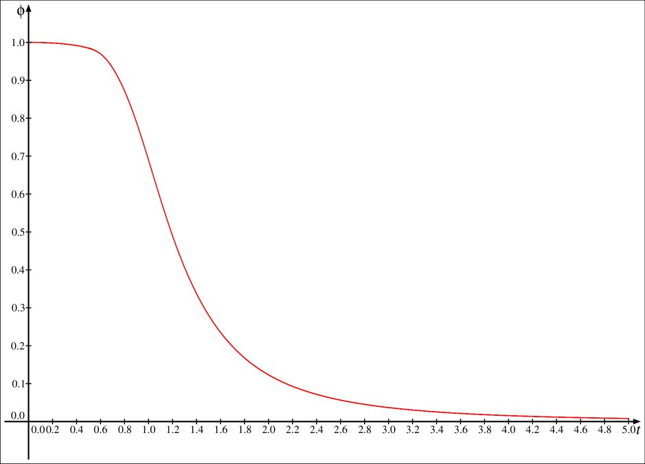
Figure 1. The function $\phi$. For $0\leq t\leq 0.5$, the power series was used, for $0.5\leq t\leq 2$ the sum, and for $t\geq 2$ the functional equation.

Note that for $t\to 0$,

$$\phi(t) =1-\frac{1}{2^{3}\cdot 3}\,t^{2}-\frac{19}{2^{7}\cdot 3}\,t^{4}-\frac{217}{2^{10}\cdot 3}\,t^{6}-\frac{9583}{2^{15}\cdot 3}\,t^{8}-\frac{40125}{2^{18}}\,t^{10}+O(t^{12})\,,$$

so that we can extend $\phi$ to all of ${\mathbb{R}}$ by setting $\phi(0)=1$ and $\phi(t)=\phi(|t|)$. The power series expansion is obtained by noting that for $|t|\leq 1/2$, we have

$$\varepsilon_{0}+\varepsilon_{1}t+\dots+\varepsilon_{6}t^{6}\geq 0\quad\iff\quad\varepsilon_{0}=+1\,.$$

The radius of convergence of the series is given by the positive root $\rho\approx 0.504138$ of $1-t-t^{2}-\dots-t^{6}$. We have the functional equation (for $t\neq 0$)

$$\phi\Bigl{(}\frac{1}{t}\Bigr{)}=t^{3}\,\phi(t)\,.$$

Furthermore, $\phi(t)$ is decreasing for $t\geq 0$. This implies that

$$\frac{\phi(1)}{H(a:b)^{3}}\leq\gamma(a:b)\leq\frac{1}{H(a:b)^{3}}\,.$$

Note that

$$\phi(1)=\frac{7^{13/2}-7\cdot 5^{13/2}+21\cdot 3^{13/2}-35}{135135}\approx 0.689540287634369059265\,.$$

See Figure 1 for a graph of $\phi$.

We postpone the proof of the claim (2.1) to Section 3.

Summing the terms for $H(a:b)\leq H$, we obtain, denoting by ${\mathbb{E}}_{\leq H}(N)$ the average number of rational points of height $\leq H$ (where the height of a rational point is the usual naive height $H(a:b)=\max\{|a|,|b|\}$ of its $x$-coordinate $(a:b)$):

$${\mathbb{E}}_{\leq H}(N)\sim\frac{\gamma_{H}}{\sqrt{N}}\qquad\text{as $N\to\infty$, uniformly for $H\ll N^{6/5-\varepsilon}$},$$

where

$$\gamma_{H}=\sum_{H(a:b)\leq H}\gamma(a:b)\,.$$

See Cor. 8 in Section 3 below.

We obtain Conjecture 1 by letting $H\to\infty$, with

$$\gamma=\lim_{H\to\infty}\gamma_{H}=\sum_{(a:b)\in{\mathbb{P}}^{1}({\mathbb{Q}})}\gamma(a:b)\,.$$

We denote by ${\mathbb{E}}(N)$ the average number of rational points on curves in ${\mathcal{C}}_{N}$. Note that we can at least prove the following (which is, however, the less interesting inequality).

Proposition 5.

We have

$$\liminf_{N\to\infty}\sqrt{N}\,{\mathbb{E}}(N)\geq\gamma\,.$$

Proof.

Given $\varepsilon>0$, fix $H$ such that $\gamma_{H}>\gamma-\varepsilon$. We then have

$$\sqrt{N}\,{\mathbb{E}}(N)\geq\sqrt{N}\,{\mathbb{E}}_{H}(N)>\gamma_{H}-\varepsilon>\gamma-2\varepsilon\qquad\text{for $N$ sufficiently large.}$$

∎

In order to prove Conjecture 1, one would need a reasonably good estimate for the number of very large points. This is most likely a very hard problem.

Let us look a bit closer at the value of $\gamma$. We have

$$\gamma=4\sum_{b=1}^{\infty}\mathop{\sum\nolimits^{\prime}}_{0\leq a\leq b,a\perp b}\frac{1}{b^{3}}\phi\Bigl{(}\frac{a}{b}\Bigr{)}=\frac{4}{\zeta(3)}\sum_{H=1}^{\infty}\frac{1}{H^{3}}\mathop{\sum\nolimits^{\prime}}_{0\leq a\leq H}\phi\Bigl{(}\frac{a}{H}\Bigr{)}\,.$$

Here, $\sum^{\prime}$ denotes the sum with first and last terms counted half.

By the Euler-Maclaurin summation formula,

$$\mathop{\sum\nolimits^{\prime}}_{0\leq a\leq H}\phi\Bigl{(}\frac{a}{H}\Bigr{)}=H\int_{0}^{1}\phi(t)\,dt+\frac{1}{12H}\phi^{\prime}(1)-\frac{1}{720H^{3}}\phi^{\prime\prime\prime}(1)+O\Bigl{(}\frac{1}{H^{5}}\Bigr{)}\,.$$

So we obtain

$$\gamma=4\Bigl{(}\frac{\zeta(2)}{\zeta(3)}\int_{0}^{1}\phi(t)\,dt+\frac{\phi^{\prime}(1)\zeta(4)}{12\zeta(3)}-\frac{\phi^{\prime\prime\prime}(1)\zeta(6)}{240\zeta(3)}+R\Bigr{)}\,,$$

with a small error $R$.

For more precise numerical estimates, we compute the first few terms in the series over $H$ to some precision and estimate the tail of the series by the formula above. Note that the derivatives of $\phi$ at $t=1$ can be computed explicitly. We find

$$\gamma\approx 4.79991101188445188\,.$$

Here is a table with experimental data obtained from all curves of size $N\leq 10$. For $N\leq 3$, the number of points should be accurate; for $4\leq N\leq 10$, we counted all points of height up to $2^{14}-1$, so the numbers given are lower bounds. However, the difference is likely to be so small that it does not affect the leading few digits. See Section 7 for the source of these data.

size of curves $\leq N$	1	2	3	4	5	6	7	8	9	10
avg. $\#C({\mathbb{Q}})$	3.94	2.70	2.19	2.42	2.08	1.84	1.66	1.52	1.65	1.53
(avg. $\#C({\mathbb{Q}})$)$\sqrt{N}$	3.94	3.82	3.79	4.84	4.66	4.50	4.40	4.31	4.94	4.83

We observe values reasonably close to the expected asymptotic value $\gamma\approx 4.800$. When $N$ is a square, the average number of points jumps up because of the additional possibilities for points at $x=0$ or $x=\infty$ (leading or trailing coefficient equal to $N$).

From the above, we also get an estimate for $\gamma-\gamma_{H}$:

$$\gamma-\gamma_{H}=4\sum_{b>H}\sum_{0<a<b,a\perp b}\frac{1}{b^{3}}\phi\Bigl{(}\frac{a}{b}\Bigr{)}\approx\frac{4}{\zeta(2)H}\int_{0}^{1}\phi(t)\,dt\approx 2.28253672259903912\,\frac{1}{H}\,.$$

3. Proof of the asymptotics for fixed $(a:b)$

The total number of rational points with $x$-coordinate $(a:b)\in{\mathbb{P}}^{1}({\mathbb{Q}})$ on curves in ${\mathcal{C}}_{N}\cup{\mathcal{D}}_{N}$ is the number of integral solutions $(f_{0},f_{1},\dots,f_{6},y)$ of the equation

$$f_{6}a^{6}+f_{5}a^{5}b+f_{4}a^{4}b^{2}+f_{3}a^{3}b^{3}+f_{2}a^{2}b^{4}+f_{1}ab^{5}+f_{0}b^{6}=y^{2}\,,$$

subject to the inequalities $-N\leq f_{j}\leq N$ for $j=0,1,\dots,6$. If we fix $y$, then the solutions correspond to the lattice points in the intersection of the cube $[-N,N]^{7}$ with the hyperplane given by the equation above. For $y=0$, the intersection of ${\mathbb{Z}}^{7}$ with the hyperplane, which we will denote $L_{(a:b)}$, is spanned by the vectors

$$(-a,b,0,0,0,0,0),(0,-a,b,0,0,0,0),\dots,(0,0,0,0,-a,b,0),(0,0,0,0,0,-a,b)\,.$$

We can define the lattice spanned by these vectors for any $(a:b)\in{\mathbb{P}}^{1}({\mathbb{R}})$. These lattices (considered up to scaling) make up the image of the obvious map from ${\mathbb{P}}^{1}({\mathbb{R}})$ into the moduli space of $6$-dimensional lattices; this image is compact since ${\mathbb{P}}^{1}({\mathbb{R}})$ is. This implies that all invariants of our lattices (like for example the covering radius) can be estimated above and below by a constant times a suitable power of the typical length $H(a:b)$ associated to the lattice. For some of these invariants, we give explicit bounds below.

The Gram matrix of the vectors above is tridiagonal:

$$\begin{pmatrix}a^{2}+b^{2}&-ab&0&\cdots&0\\ -ab&a^{2}+b^{2}&-ab&\cdots&0\\ 0&-ab&a^{2}+b^{2}&\cdots&0\\ \vdots&\vdots&\vdots&\ddots&\vdots\\ 0&0&0&\cdots&a^{2}+b^{2}\end{pmatrix}$$

(From this matrix, one can again see that the lattice has a nearly orthogonal basis consisting of vectors of equal length.) The covolume of the lattice (in six-dimensional volume in ${\mathbb{R}}^{7}$) is

$$\Delta_{(a:b)}=\sqrt{a^{12}+a^{10}b^{2}+\dots+b^{12}}\,;$$

we have

$$H(a:b)^{6}\leq\Delta_{(a:b)}\leq\sqrt{7}H(a:b)^{6}.$$

The diameter of the fundamental parallelotope spanned by these vectors is

$$\delta_{(a:b)}=\sqrt{a^{2}+5(|a|+|b|)^{2}+b^{2}}=\sqrt{6a^{2}+10|ab|+6b^{2}}\leq\sqrt{22}\,H(a:b)\,.$$

Let

$$\mathbf{a}_{(a:b)}=(b^{6},ab^{5},a^{2}b^{4},\dots,a^{6})\in{\mathbb{R}}^{7}$$

and

$$\mathbf{e}_{(a:b)}=\frac{1}{\Delta_{(a:b)}^{2}}\,\mathbf{a}_{(a:b)}$$

(note that $\mathbf{a}_{(a:b)}\cdot\mathbf{e}_{(a:b)}=1$); then the number of points we want to count is

$$\sum_{y\in{\mathbb{Z}}}\#\bigl{(}{\mathbb{Z}}^{7}\cap[-N,N]^{7}\cap(L_{(a:b)}+y^{2}\mathbf{e}_{(a:b)})\bigr{)}=\sum_{y\in{\mathbb{Z}}}\#S(y)\,,$$

where we define $S(y)$ to be the set under the ‘$\#$’ sign in the first sum. Let $V_{(a:b)}\subset L_{(a:b)}$ be the Voronoi cell of the lattice ${\mathbb{Z}}^{7}\cap L_{(a:b)}$; in particular it has volume $\Delta_{(a:b)}$, and its translates by lattice points tessellate $L_{(a:b)}$. We consider $S(y)+V_{(a:b)}$. The (6-dimensional) volume of this set is $\#S(y)\Delta_{(a:b)}$. We use $B_{r}(x)$ to denote the closed ball of radius $r$ with center $x$. Write

$$W_{(a:b)}(t,\delta)=\begin{cases}\bigl{\{}x\in L_{(a:b)}+t\mathbf{e}_{(a:b)}:B_{-\delta(x)}\subset[-1,1]^{7}\bigr{\}}\,,&\text{if $\delta\leq 0$,}\\ \bigl{\{}x\in L_{(a:b)}+t\mathbf{e}_{(a:b)}:B_{\delta}(x)\cap[-1,1]^{7}\neq\emptyset\bigr{\}}\,,&\text{if $\delta\geq 0$.}\end{cases}$$

In particular, $W_{(a:b)}(t,0)=(L_{(a:b)}+t\mathbf{e}_{(a:b)})\cap[-1,1]^{7}$.

There is a constant $c_{0}>0$ such that the covering radius of the lattice ${\mathbb{Z}}^{7}\cap L_{(a:b)}$ is bounded by $c_{0}H(a:b)$ (see the remark above). Writing $H=H(a:b)$ in the following, we obtain

$$N\cdot W_{(a:b)}\Bigl{(}\frac{y^{2}}{N},-\frac{c_{0}H}{N}\Bigr{)}\subset S(y)+V_{(a:b)}\subset N\cdot W_{(a:b)}\Bigl{(}\frac{y^{2}}{N},\frac{c_{0}H}{N}\Bigr{)}\,.$$

Since

$$\operatorname{vol}_{6}W_{(a:b)}(t,\delta)=\operatorname{vol}_{6}W_{(a:b)}(t,0)+O(\delta)+O(\delta^{6})$$

(with $O$-constants independent of $(a:b)$), we obtain

$$\#S(y)\Delta_{(a:b)}=N^{6}\,\operatorname{vol}_{6}W_{(a:b)}\Bigl{(}\frac{y^{2}}{N},0\Bigr{)}+O(HN^{5})+O(H^{6})\,.$$

Therefore, using that $\Delta_{(a:b)}\asymp H^{6}$ and writing $f_{(a:b)}(t)=\operatorname{vol}_{6}W_{(a:b)}(t,0)$,

$$\#S(y)=\frac{N^{6}}{\Delta_{(a:b)}}f_{(a:b)}\Bigl{(}\frac{y^{2}}{N}\Bigr{)}+O(H^{-5}N^{5})+O(1)\,.$$

Let $S(a:b)$ be the set $\cup_{y\in{\mathbb{Z}}}S(y)$ of all relevant lattice points. Then

$$\#S(a:b) =\sum_{y\in{\mathbb{Z}}}\#S(y)$$

$$=\frac{N^{6}}{\Delta_{(a:b)}}\sum_{y\in{\mathbb{Z}}}f_{(a:b)}\Bigl{(}\frac{y^{2}}{N}\Bigr{)}+O(H^{-2}N^{11/2})+O(H^{3}N^{1/2})$$

$$=\frac{2N^{6}}{\Delta_{(a:b)}}\int_{0}^{\infty}f_{(a:b)}\Bigl{(}\frac{y^{2}}{N}\Bigr{)}\,dy\,+O(H^{-6}N^{6})+O(H^{-2}N^{11/2})+O(H^{3}N^{1/2})\,.$$

(Note that $y=O(\sqrt{N\Delta_{(a:b)}})=O(H^{3}\sqrt{N})$ and that $f_{(a:b)}(t)$ is decreasing for $t\geq 0$, with $f(0)=O(1)$.) Substituting $t=y^{2}/N$, this gives

$$\#S(a:b) =\frac{N^{13/2}}{\Delta_{(a:b)}}\int_{0}^{\infty}f_{(a:b)}(t)\,\frac{dt}{\sqrt{t}}+O(H^{-6}N^{6})+O(H^{-2}N^{11/2})+O(H^{3}N^{1/2})$$

$$=N^{13/2}\int_{[-1,1]^{7}}(\mathbf{a}_{(a:b)}\cdot\mathbf{x})_{+}^{-1/2}\,d\mathbf{x}$$

$$\qquad\qquad{}+O(H^{-6}N^{6})+O(H^{-2}N^{11/2})+O(H^{3}N^{1/2})\,.$$

Here $x_{+}^{-1/2}$ is zero when $x\leq 0$ and $x^{-1/2}$ when $x>0$. More generally, for $x,r\in{\mathbb{R}}$, we let $x_{+}^{r}$ denote $0$ when $x\leq 0$ and $x^{r}$ when $x>0$.

Lemma 6.

We have, for $ab\neq 0$,

$$\int_{[-1,1]^{7}} (\mathbf{a}_{(a:b)}\cdot\mathbf{x})_{+}^{-1/2}\,d\mathbf{x}$$

$$=\frac{2^{7}}{135135\,|ab|^{21}}\!\sum_{\varepsilon_{0},\dots,\varepsilon_{6}=\pm 1}\!\varepsilon_{0}\cdots\varepsilon_{6}(\varepsilon_{0}|b^{6}|+\varepsilon_{1}|ab^{5}|+\dots+\varepsilon_{6}|a^{6}|)_{+}^{13/2}.$$

Note that this is $2^{7}$ times

$$\gamma(a:b)=\frac{1}{|b|^{3}}\phi\Bigl{(}\frac{|a|}{|b|}\Bigr{)}$$

in the notation introduced in the previous section.

Proof.

Let $a_{1},\dots,a_{m}>0$ be real numbers, $r>-1$, $c\in{\mathbb{R}}$. Write $\mathbf{a}=(a_{1},\dots,a_{m})$. We prove the more general statement

$$\int_{[-1,1]^{m}} (\mathbf{a}\cdot\mathbf{x}+c)_{+}^{r}\,d\mathbf{x}$$

$${}=\frac{1}{a_{1}\cdots a_{m}\,(r+1)\cdots(r+m)}\sum_{\varepsilon_{1},\dots,\varepsilon_{m}=\pm 1}\varepsilon_{1}\cdots\varepsilon_{m}(\varepsilon_{1}a_{1}+\dots+\varepsilon_{m}a_{m}+c)_{+}^{r+m}\,.$$

We proceed by induction. When $m=1$, we have

$$\int_{-1}^{1}(a_{1}x_{1}+c)_{+}^{r}\,dx_{1}=\frac{1}{a_{1}\,(r+1)}\bigl{(}(a_{1}+c)_{+}^{r+1}-(-a_{1}+c)_{+}^{r+1}\bigr{)}\,,$$

as can be checked by considering the cases $-c\leq-a_{1}$, $-a_{1}\leq-c\leq a_{1}$, and $a_{1}\leq-c$ separately.

For the inductive step, we assume the statement to be true for $a_{1},\dots,a_{m}$ and $r$, and prove it for $a_{1},\dots,a_{m},a_{m+1}$. Let $\mathbf{a}^{\prime}=(a_{1},\dots,a_{m})$ and $\mathbf{a}=(a_{1},\dots,a_{m+1})$, and use similar notation for vectors $\mathbf{x}$, $\mathbf{x}^{\prime}$. Then

$$\int_{[-1,1]^{m+1}}(\mathbf{a}\cdot\mathbf{x}+c)_{+}^{r}\,d\mathbf{x}$$

$$=\int_{-1}^{1}\int_{[-1,1]^{m}}\bigl{(}\mathbf{a}^{\prime}\cdot\mathbf{x}^{\prime}+a_{m+1}x_{m+1}+c\bigr{)}_{+}^{r}\,d\mathbf{x}^{\prime}\,dx_{m+1}$$

$$=\int_{-1}^{1}\frac{1}{a_{1}\cdots a_{m}\,(r+1)\cdots(r+m)}\times{}$$

$$\quad\sum_{\varepsilon_{1},\dots,\varepsilon_{m}=\pm 1}\varepsilon_{1}\cdots\varepsilon_{m}\bigl{(}\varepsilon_{1}a_{1}+\dots+\varepsilon_{m}a_{m}+x_{m+1}a_{m+1}+c\bigr{)}_{+}^{r+m}\,dx_{m+1}$$

$$=\frac{1}{a_{1}\cdots a_{m}\,(r+1)\cdots(r+m)}\times{}$$

$$\quad\sum_{\varepsilon_{1},\dots,\varepsilon_{m}=\pm 1}\varepsilon_{1}\cdots\varepsilon_{m}\int_{-1}^{1}\bigl{(}\varepsilon_{1}a_{1}+\dots+\varepsilon_{m}a_{m}+x_{m+1}a_{m+1}+c\bigr{)}_{+}^{r+m}\,dx_{m+1}$$

$$=\frac{1}{a_{1}\cdots a_{m}\,(r+1)\cdots(r+m)}\times{}$$

$$\quad\sum_{\varepsilon_{1},\dots,\varepsilon_{m}=\pm 1}\varepsilon_{1}\cdots\varepsilon_{m}\frac{1}{a_{m+1}\,(r+m+1)}\sum_{\varepsilon_{m+1}=\pm 1}\bigl{(}\varepsilon_{1}a_{1}+\dots+\varepsilon_{m+1}a_{m+1}+c\bigr{)}_{+}^{r+m+1}$$

by the case $m=1$.

To finish the proof of the lemma, note that we can take $a,b>0$. We then apply the claim with $\mathbf{a}=\mathbf{a}_{(a:b)}$, $r=-1/2$, and $c=0$. ∎

Corollary 7.

With $H=H(a:b)$,

$${\mathbb{E}}_{(a:b)}(N)=\frac{\gamma(a:b)}{\sqrt{N}}+O\bigl{(}H^{-6}N^{-1}\bigr{)}+O\bigl{(}H^{-2}N^{-3/2}\bigr{)}+O\bigl{(}H^{3}N^{-13/2}\bigr{)}\,.$$

In particular, we have

$$\sqrt{N}\,{\mathbb{E}}_{(a:b)}(N)\longrightarrow\gamma(a:b)$$

as $N\to\infty$, uniformly for $(a:b)$ such that $H(a:b)\ll N^{2-\varepsilon}$.

Proof.

First note that ${\mathbb{E}}_{(a:b)}(N)=\#S^{\prime}(a:b)/\#{\mathcal{C}}_{N}$, where $S^{\prime}(a:b)$ only lists the points in $S(a:b)$ on curves that are smooth. We have

$$\#{\mathcal{C}}_{N}=(2N+1)^{7}-\#{\mathcal{D}}_{N}=(2N+1)^{7}+O(N^{5})=(2N)^{7}\bigl{(}1+O(N^{-1})\bigr{)}$$

and

$$\#S^{\prime}(a:b)=\#S(a:b)+O\bigl{(}H^{-10}N^{5}\bigr{)}+O\bigl{(}H^{-1}N^{9/2}\bigr{)}+O\bigl{(}H^{3}N^{1/2}\bigr{)}\,.$$

See Section 4 below. This implies that

$${\mathbb{E}}_{(a:b)}(N)=\frac{\#S(a:b)}{(2N)^{7}}\bigl{(}1+O(N^{-1})\bigr{)}+O\bigl{(}H^{-10}N^{-2}\bigr{)}+O\bigl{(}H^{-1}N^{-5/2}\bigr{)}+O\bigl{(}H^{3}N^{-13/2}\bigr{)}\,.$$

By Lemma 6, the definition of $\gamma(a:b)$, and the discussion preceding the lemma, we have (using $\gamma(a:b)\asymp H^{-3}$)

$$\frac{\#S(a:b)}{(2N)^{7}}=\frac{\gamma(a:b)}{\sqrt{N}}+O\bigl{(}H^{-6}N^{-1}\bigr{)}+O\bigl{(}H^{-2}N^{-3/2}\bigr{)}+O\bigl{(}H^{3}N^{-13/2}\bigr{)}\,.$$

The result is obtained by combining these results, after eliminating redundant terms. ∎

Corollary 8.

$${\mathbb{E}}_{\leq H}(N)=\frac{\gamma_{H}}{\sqrt{N}}+O\bigl{(}N^{-1}\bigr{)}+O\bigl{(}(\log H)N^{-3/2}\bigr{)}+O\bigl{(}H^{5}N^{-13/2}\bigr{)}\,.$$

In particular, we have

$$\sqrt{N}\,{\mathbb{E}}_{\leq H(N)}(N)\longrightarrow\gamma_{H(N)}$$

as $N\to\infty$ if $H(N)\ll N^{6/5-\varepsilon}$, and

$${\mathbb{E}}_{\leq H(N)}(N)\longrightarrow 0$$

as $N\to\infty$ if $H(N)\ll N^{13/10-\varepsilon}$.

Proof.

Sum the estimates in the previous corollary. ∎

It should be possible to extend the range beyond $H\ll N^{6/5-\varepsilon}$ if one uses more sophisticated methods from analytic number theory. (In fact, Stephan Baier [Bai] has obtained an exponent of $7/5-\varepsilon$.) It would be interesting to see how far one can get.

4. Counting Bad Curves and Points

In this section, we will bound the number $\#{\mathcal{D}}_{N}$ of non-smooth curves and the total number of points of height $\leq H$ on them. Recall the following.

Lemma 9.

Let $\Lambda\subset{\mathbb{R}}^{n}$ be a lattice of covolume $\Delta$ and covering radius $\rho$. Let $S\subset{\mathbb{R}}^{n}$ be a subset. Then

$$\#(S\cap\Lambda)\leq\frac{\operatorname{vol}(S+B_{\rho}(0))}{\Delta}\,.$$

Proof.

Let $V$ be the Voronoi cell of $\Lambda$ (centered at zero), then $V\subset B_{\rho}(0)$ by definition of the covering radius, and $\operatorname{vol}V=\Delta$. It follows that

$$\bigcup_{x\in S\cap\Lambda}(V+x)\subset S+B_{\rho}(0)\,,\quad\text{and thus}\quad\Delta\cdot\#(S\cap\Lambda)\leq\operatorname{vol}(S+B_{\rho}(0))\,.$$

∎

To make life a bit simpler, we observe that $[-N,N]^{7}\subset B_{\sqrt{7}N}(0)$; we will bound the number of bad curves in the ball. This has the advantage that the intersection with any affine subspace will be a ball again.

Note that a form $F(x,z)$ is not square-free if and only if it is divisible by the square of a primitive form $G$. Let $n$ be the degree of $G$; assume it has coefficients $\boldsymbol{\alpha}=(\alpha_{n},\dots,\alpha_{0})$. Then the forms divisible by $G^{2}$ correspond to lattice points in the span of

$$x^{6-2n}G^{2}\,,x^{5-2n}zG^{2}\,,\dots\,,z^{6-2n}G^{2}\,,$$

intersected with the ball $B_{\sqrt{7}N}(0)$.

We can extend this to $G$ with real coefficients; then the lattices we obtain (modulo scaling) are parametrized by the compact set ${\mathbb{P}}^{n}({\mathbb{R}})$, hence they all live in a compact subset of the moduli space of lattices. Taking into account that the basis vectors have length of order $H(\boldsymbol{\alpha})^{2}$, this gives the following relations for the covolume, covering radius and minimal length of the lattices.

$$\Delta\asymp H(\boldsymbol{\alpha})^{14-4n}\,,\qquad\rho\asymp H(\boldsymbol{\alpha})^{2}\,,\qquad\mu\asymp H(\boldsymbol{\alpha})^{2}\,.$$

In particular, there will be no non-zero lattice point in the ball of radius $\sqrt{7}N$ when $N>\text{const}\,H(\boldsymbol{\alpha})^{2}$. By Lemma 9, we then obtain a bound

$$\#{\mathcal{D}}_{N} \leq\sum_{n=1}^{3}\sum_{\boldsymbol{\alpha}\in{\mathbb{P}}^{n}({\mathbb{Q}}),H(\boldsymbol{\alpha})\ll\sqrt{N}}O\Bigl{(}\frac{(N+H(\boldsymbol{\alpha})^{2})^{7-2n}}{H(\boldsymbol{\alpha})^{14-4n}}\Bigr{)}$$

$$=\sum_{n=1}^{3}\sum_{\boldsymbol{\alpha}\in{\mathbb{P}}^{n}({\mathbb{Q}}),H(\boldsymbol{\alpha})\ll\sqrt{N}}O\Bigl{(}\frac{N^{7-2n}}{H(\boldsymbol{\alpha})^{14-4n}}\Bigr{)}$$

$$=\sum_{n=1}^{3}N^{7-2n}\sum_{H\ll\sqrt{N}}O(H^{3n-14})=O(N^{5})\,.$$

We conclude that in fact $\#{\mathcal{D}}_{N}\asymp N^{5}$, since we already get $N^{5}$ from $G=x$.

Now in order to count points on these bad curves, we use the same basic idea as before. This time, we have to count lattice points in the ball that are in a translate of the subspace of forms that are divisible by $G(x,z)^{2}(bx-az)$. We assume for now that $G(a,b)\neq 0$. If $F(a,b)=G(a,b)^{2}y^{2}$, then the translation is by a vector of length $G(a,b)^{2}y^{2}/\Delta_{(a:b)}$. So for the count of points with $x$-coordinate $(a:b)$, we get a bound of

$$\sum_{|y|\ll\frac{\sqrt{N\Delta_{(a:b)}}}{|G(a,b)|}}O\Bigl{(}\frac{(N+H(\boldsymbol{\alpha})^{2})^{6-2n}}{H(\boldsymbol{\alpha})^{12-4n}H(a:b)^{6-2n}}\Bigr{)}=O\Bigl{(}\frac{N^{\frac{13}{2}-2n}}{|G(a,b)|H(\boldsymbol{\alpha})^{12-4n}H(a:b)^{3-2n}}\Bigr{)}\,.$$

Estimating $|G(a,b)|\geq 1$ trivially, we obtain for the total number of such points the bound

$$\sum_{n=1}^{3} \sum_{H(\boldsymbol{\alpha})\ll\sqrt{N}}O\Bigl{(}\frac{N^{\frac{13}{2}-2n}}{H(\boldsymbol{\alpha})^{12-4n}H(a:b)^{3-2n}}\Bigr{)}$$

$$=O\Bigl{(}\frac{N^{9/2}}{H(a:b)}\Bigr{)}+O\bigl{(}N^{5/2}H(a:b)\bigr{)}+O\bigl{(}N^{1/2}H(a:b)^{3}\bigr{)}\,.$$

The middle term is redundant, since it is always dominated by one of the others.

If $G(a,b)=0$, then (since we can assume $G$ to be irreducible) $n=1$, and we have to count all forms divisible by $G^{2}$. This adds a term of order $N^{5}/H(a:b)^{10}$.

Remark 10.

With a similar computation as above, one can show that the number of curves in ${\mathcal{C}}_{N}$ with reducible polynomial $F$ is $O(N^{6})$. Therefore the contribution of such curves is negligible.

5. Speculations on the Size of Points

Recall that

$$\gamma_{H}\approx\gamma-\frac{c}{H}$$

where $c\approx 2.28253672259903912$. If we assume Conj. 1, then the calculations above suggest that the number of curves in ${\mathcal{C}}_{N}$ that have a rational point of $x$-height $>H$ is roughly $cN^{13/2}/H$, at least as long as $H$ is not too large compared to $N$, see Cor. 8. If we recklessly extend this to large $H$, this would predict that the largest rational point on a curve from ${\mathcal{C}}_{N}$ should have height $\ll N^{13/2+\varepsilon}$. One has to be careful, however, as was pointed out to me by Noam Elkies, mentioning the case of integral points on elliptic curves as an analogy. Considering curves in short Weierstrass form $y^{2}=x^{3}+Ax+B$ with $A,B\in{\mathbb{Z}}$, heuristic considerations like those presented here predict that integral points should be of size $\ll\max\{|A|^{1/2},|B|^{1/3}\}^{10+\varepsilon}$, but there are families that reach an exponent of $12$. See the information given at [El1]. This leads to Conjecture 2.

Regarding possible families with larger points, we consider the case that the coefficients $f_{j}$ are linear forms in the coordinates $(t:u)$ of ${\mathbb{P}}^{1}$, the coordinates $x$ and $z$ of the point we are looking for are homogeneous polynomials of degree $m$ (to be determined), and $y^{2}=q(t,u)^{2}r(t,u)$ with $q$ of degree $3m-1$ and $r$ of degree $3$. If we find a solution of

$$q^{2}r=\sum_{j=0}^{6}f_{j}x^{j}z^{6-j}$$

in such polynomials, then we should obtain an infinite family of curves with points satisfying $H(P)\gg N^{m}$. (Of course, we have to exclude degenerate solutions.) To see this, multiply by $r(1,0)$ (which we can assume to be nonzero after a suitable change of coordinates on ${\mathbb{P}}^{1}$). The equation

$$r(1,0)r(t,u)=w^{2}$$

then has the solution $(t,u,w)=(1,0,r(1,0))$, which must be contained in a family of solutions that is parametrized by a genus $0$ curve (compare [DG, Beu]). If we plug in this parametrization, we obtain a one-dimensional family of suitable curves with base ${\mathbb{P}}^{1}$.

There are

$$3m+4+7\cdot 2+2\cdot(m+1)=5m+20$$

unknown coefficients involved in the equation above. On the other hand, there is an action of $\operatorname{GL}_{2}\times\operatorname{GL}_{2}\times{\mathbb{G}}_{\text{\rm m}}$ (given by the automorphisms of ${\mathbb{P}}^{1}_{(t:u)}$, the automorphisms of ${\mathbb{P}}^{1}_{(x:z)}$ (acting on $x$, $z$, and the $f_{j}$ and leaving the value of the right hand side unchanged), and scaling of $q$ versus $r$), which takes away 9 degrees of freedom. The relation above leads to $6m+2$ equations, so the remaining number of degrees of freedom should be

$$(5m+20)-9-(6m+2)=9-m\,.$$

This suggests that there should be families of curves with points such that $H(P)\gg N^{9}$. (We do not get better results when we take coefficients $f_{j}$ of higher degree, taking $\deg r=4$ in case this degree is even.) Of course, the corresponding variety may fail to have rational points, so that we do not see these families over ${\mathbb{Q}}$. Or some other accidents can occur, leading to extraneous solutions with larger $m$.

In the following, we will ignore such special families and try to make our ‘generic’ conjecture more precise by using a probabilistic model. In this model, we interpret the quantity

$$\frac{N^{6}}{\Delta_{(a:b)}}\int_{0}^{\infty}f_{(a:b)}\Bigl{(}\frac{y^{2}}{N}\Bigr{)}\,dy=2^{6}\gamma(a:b)N^{13/2}$$

that gives rise to the main term in the count of points $(a:\pm y:b)$ as the probability that such a point pair occurs in ${\mathcal{C}}_{N}$. The number of pairs of points of height $>H$ should then follow a Poisson distribution with mean

$$\mu_{H}=2^{6}(\gamma-\gamma_{H})N^{13/2}\approx\frac{2^{6}cN^{13/2}}{H}\,,$$

at least when $H$ is large compared to $N$. Taking $H=\lambda N^{13/2}$, the probability that no such point exists is then $e^{-2^{6}c/\lambda}$. Taking into account the fact that points occur in packets of eight (change the sign of $x$ or $y$, send $x$ to $1/x$), i.e., four point pairs, we should correct this to $e^{-16c/\lambda}$. For a fifty-fifty chance of no larger points, we should take $\lambda\approx 53$, for an 80% chance, we take $\lambda\approx 164$. This line of argument would lead us to expect the following.

If $\lambda(N)\to\infty$ as $N\to\infty$, then there are only finitely many ‘generic’ curves $C\in{\mathcal{C}}_{N}$ of genus 2 such that $C$ has a rational point $P$ with $H(P)>\lambda(N)N^{13/2}$.

The problem with this is that it is not so clear how to make the restriction to ‘generic’ curves precise. There might be an infinity of families of curves with points of height $N^{k}$ for a sequence of $k$ tending to $13/2$ from above, which could lead to problems when $\lambda(N)$ tends to infinity very slowly. Therefore, we keep on the safe side with the given formulation of Conjecture 2.

On the other hand, we can use similar heuristic arguments for any given family of curves. It is reasonable to expect that the bounds we obtain will not get arbitrarily large (in terms of the exponent of $N$ in the height bound). This leads to Conjecture 3.

We have checked experimentally how well the expected number of points of height in the interval $\left[2^{n},2^{n+1}\right[$ matches the actual number of points on curves of small size. For values of $n$ that are not very small, this is $2^{-(n+1)}c\,\#{\mathcal{C}}_{N}/\sqrt{N}$. Figure 2 shows this comparison, for curves in ${\mathcal{C}}_{N}$, for $1\leq N\leq 10$ and $0\leq n\leq 13$. The fit is quite good, even though the range of $N$ is certainly far too small for the asymptotics to kick in except for very small heights. There is an unexpected feature: starting with $N=4$, points of larger height seem to occur more frequently than they should. It would be interesting to find an explanation for this phenomenon. One possibility is that it might be related to the existence of families of curves with systematically occurring large points. Of course, according to our results, this can only occur for fairly large heights when $N$ is large. See Section 7 for a description of the computations.

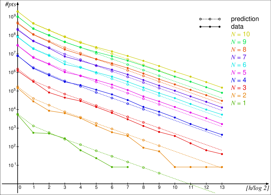
Figure 2. Expected and actual number of rational points in various height brackets, for $1\leq N\leq 10$.

It is also interesting to compare the observed value of $\lambda(N)$ such that no rational point of height $>\lambda(N)N^{13/2}$ exists on a curve in ${\mathcal{C}}_{N}$ with the estimates given above. For $N=1,2,3$, the largest points we found on curves in ${\mathcal{C}}_{N}$ have heights as follows.

size of curves	$N=1$	$N=2$	$N=3$
max. $H(P)$	145	10711	209040

We therefore find

$$\lambda(1)\approx 145.00\,,\quad\lambda(2)\approx 118.34\,,\quad\lambda(3)\approx 165.55\,,$$

corresponding to probabilities (for no larger point to exist, in the sense explained above) between 73% and 81%.

The record point on  $y^{2}=x^{6}-3x^{4}-x^{3}+3x^{2}+3$  has $x=-\frac{58189}{209040}$.

Similar considerations for general hyperelliptic curves of genus $g\geq 2$ lead to a heuristic estimate of $O(N^{(4g+5)/2}/H^{g-1})$ for the number of curves with a point of height $>H$. Therefore we would expect the points to be generically of height

$$H\ll N^{(4g+5)/(2g-2)+\varepsilon}=N^{2+\frac{9}{2(g-1)}+\varepsilon}\,.$$

6. Speculations on the Number of Points

We can also try to extract some information of the number of points (or point pairs) on hyperelliptic curves. Since the linear conditions on the coefficients coming from up to seven distinct $x$-coordinates are linearly independent, we would expect the following.

Let $R^{(m)}_{N}$ be the subset of ${\mathcal{C}}_{N}$ of curves that have at least $m$ pairs of rational points (i.e., points with $m$ distinct $x$-coordinates). For $0\leq m\leq 7$, there are constants $\gamma^{(m)}>0$ such that

$$\#R^{(m)}_{N}\sim\gamma^{(m)}\,N^{7-m/2}\,.$$

One caveat here is that the number of non-squarefree polynomials will be in the range of these sizes if $m\geq 4$, so the conclusion is not automatic. Indeed, the experimental data show a noticeable deviation from this expectation already for $m\geq 3$.

Let us be more precise and try to obtain numerical values for the $\gamma^{(m)}$. Assuming the occurrence or not of points with distinct $x$-coordinates to be independent for all $x\in{\mathbb{P}}^{1}({\mathbb{Q}})$, the generating function for the probability of having rational points with exactly $m$ distinct $x$-coordinates should be (assuming exact probability $\gamma(a:b)/2\sqrt{N}$ for a point $P\in C({\mathbb{Q}})$ with $x(P)=(a:b)$)

$$G(T)=\sum_{m=0}^{\infty}\operatorname{Prob}_{N}\bigl{(}\#x(C({\mathbb{Q}}))=m\bigr{)}T^{m}=\prod_{(a:b)\in{\mathbb{P}}^{1}({\mathbb{Q}})}\Bigl{(}1+\frac{\gamma(a:b)}{2\sqrt{N}}(T-1)\Bigr{)}\,.$$

The numbers $\gamma^{(m)}$ should then occur as the limits as $N\to\infty$ of the coefficients in the series

$$\sum_{m=0}^{\infty}\gamma^{(m)}(N)\,T^{m}=\frac{1-\sqrt{N}T\,G(\sqrt{N}T)}{1-\sqrt{N}T}=\frac{T\,G(\sqrt{N}T)-\frac{1}{\sqrt{N}}}{T-\frac{1}{\sqrt{N}}}\,,$$

where $\gamma^{(m)}(N)N^{-m/2}$ is an estimate for the fraction of curves with at least $m$ point pairs. Now, as $N\to\infty$ and coefficient-wise, this series behaves as

$$G(\sqrt{N}T)=\prod_{(a:b)}\Bigl{(}1-\frac{\gamma(a:b)}{2\sqrt{N}}+\frac{\gamma(a:b)}{2}\,T\Bigr{)}\longrightarrow\prod_{(a:b)}\Bigl{(}1+\frac{\gamma(a:b)}{2}\,T\Bigr{)}\,.$$

So $\gamma^{(m)}$ is the degree-$m$ “infinite elementary symmetric polynomial” in the numbers $\gamma(a:b)/2$. Using $(a:b)$ of height up to $1000$, we find

$$\gamma^{(1)}=\frac{\gamma}{2}\approx 2.399\,,\quad\gamma^{(2)}\approx 2.499\,,\quad\gamma^{(3)}\approx 1.504\,,\quad\gamma^{(4)}\approx 0.591\,,\text{\quad etc.}$$

In Figure 3, we compare the expected values $\gamma^{(m)}(N)/N^{m/2}$ with the observed numbers. For $m\leq 2$, there is good agreement, but for $m\geq 4$, there seem to be many more curves with at least $m$ pairs of points than predicted. Indeed, the data suggest a behavior of the form $\alpha^{m}$ for the fraction of curves in this range, with $\alpha\approx 0.5$ largely independent of $N$ (or even increasing: note the changes in slope when $N=4$ or $N=9$).

This seems to indicate that as soon as there are many points, it is much more likely that there are additional points than on average — the points “conspire” to generate more points. Maybe this is related to another observation, which is that in examples of curves with many rational points, the points tend to have many dependence relations in the Mordell-Weil group. One possible explanation might be that when there are already several points, they tend to be fairly small, so that there are many small linear combinations of them in the Mordell-Weil group. Such a small point in the Mordell-Weil group is represented by a pair of points on $C$ such that the quadratic polynomial whose roots are the $x$-coordinates of the two points has small height. A polynomial of small height has a good chance to split into linear factors. In this case, both points involved are rational points on $C$. It would be very interesting to turn this into a precise estimate for the number $\alpha$ that we observe.

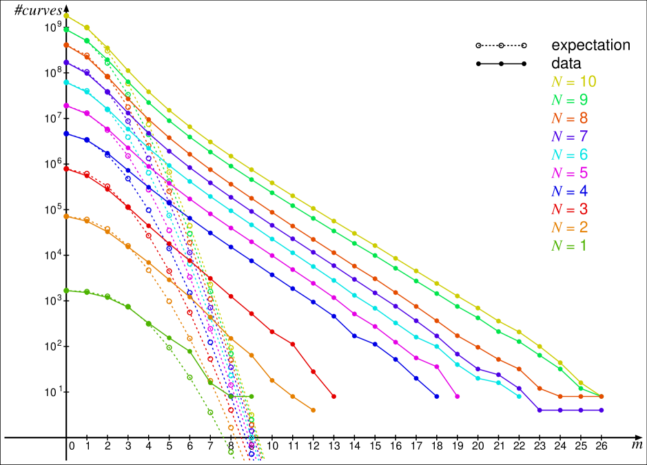
Figure 3. Expected and actual number of curves with at least $m$ pairs of rational points

In Figure 4, we show the proportion of curves in ${\mathcal{C}}_{N}$ with at least $m$ point pairs. It is striking how the graphs are all contained in a narrow strip near the line (in the logarithmic scaling used in the picture) corresponding to $m\mapsto 2^{-m}$.

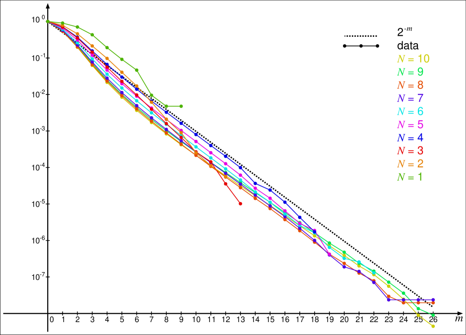
Figure 4. Proportion of curves with at least $m$ pairs of rational points

If these observations extend to larger $N$, then we should expect about $2^{-m}(2N+1)^{7}$ curves in ${\mathcal{C}}_{N}$ with $m$ or more point pairs. The largest number of point pairs on a curve in ${\mathcal{C}}_{N}$ should then be

$$\frac{7}{\log 2}\,\log(2N+1)+O(1)\,.$$

Conjecture 4 gives a slightly weaker statement, replacing the factor $7/\log 2$ by an arbitrary constant.

In order to test our conjecture, we conducted a search for curves with many points in ${\mathcal{C}}_{200}$. The table in Figure 5 lists the record curves we found (curves with more point pairs than all smaller curves). On each curve, we found all points of height up to $2^{17}-1=131\,071$ (and in some cases a few more). The column labeled “$F$” lists the coefficients of one example curve.

$$\begin{array}[]{|c|c|c|c|c|}\hline\cr N&F&\#C({\mathbb{Q}})&\frac{\#C({\mathbb{Q}})}{\log_{10}(2N+1)}\text{\LARGE}\\ \hline\cr 1&1,-1,0,1,-1,0,1&18&37.73\\ 2&1,2,0,-2,2,0,1&24&34.34\\ 3&1,-3,2,3,0,0,1&26&30.77\\ 4&4,4,0,-1,-4,0,1&36&37.73\\ 5&4,4,0,-5,-4,1,1&38&36.49\\ 6&1,6,-1,-5,0,-1,1&44&39.50\\ 7&4,-7,-5,5,1,2,1&52&44.21\\ 11&9,2,-11,-5,3,9,9&56&41.12\\ 13&9,-12,-4,13,-4,3,4&62&43.32\\ 16&4,1,-16,-13,16,8,1&68&44.78\\ 19&1,-18,-19,6,11,12,16&72&45.25\\ 20&4,3,20,5,-3,-20,16&74&45.88\\ 21&4,3,19,-21,-19,14,1&78&47.75\\ 24&9,24,-10,-20,2,-12,16&80&47.33\\ 36&9,3,-35,5,27,-20,36&82&44.01\\ 42&4,-13,23,7,-42,0,25&88&45.61\\ 47&9,-21,23,-7,-47,28,16&98&49.55\\ 54&9,-54,3,-2,-36,32,49&104&51.04\\ 66&25,-30,-37,-46,66,34,4&106&49.91\\ 67&1,-46,67,38,32,-32,4&114&53.51\\ 70&49,-60,-28,-70,-9,70,49&118&54.90\\ 72&1,2,63,-38,-72,36,9&120&55.52\\ 110&25,-32,80,110,-105,-78,49&124&52.89\\ 117&1,-26,87,83,-43,-117,64&126&53.14\\ 125&49,42,-85,-125,77,69,9&130&54.17\\ 132&81,-132,-16,71,76,-71,16&138&56.95\\ 143&81,-120,-28,-54,143,90,9&140&56.96\\ 184&1,98,-59,-184,161,46,1&142&55.32\\ 191&4,-4,156,-191,-159,171,144&146&56.52\\ \hline\cr\end{array}$$

Figure 5. Examples of curves with many points.

The constant in front of $\log(2N+1)$ that seems to fit our data best points to a value of $\alpha$ of about $0.68$ in that range (corresponding to the slope of the lines in the figure and indicating that the observed increase of $\alpha$ with $N$ persists). In Figure 6, we have plotted $\#C({\mathbb{Q}})$ against $\log(2N+1)$ for the curves in the table (and some more coming from an ongoing extended search). In addition, we show a selection of good curves from Elkies’ families, see below, and some other previously known examples. (“$\log$” in the figure is the logarithm with base $10$.) The sources of these examples are [Kul, KK, Sta]; the curve marked “Stahlke” on the left was communicated to me by Colin Stahlke; it appears in [Sto], where the Mordell-Weil group of its Jacobian is determined.

One of these examples is the curve with the largest number of point pairs found until very recently (see Keller and Kulesz [KK]). It has $N=22\,999\,624\,761$ and $m=294$. This curve has 12 automorphisms defined over ${\mathbb{Q}}$, and the 588 points are 49 orbits of 12 points each. Until 2008, the record for curves with only the hyperelliptic involution as a nontrivial automorphism was held by a curve found by Stahlke [Sta] with 366 known rational points. (In fact, there are at least 8 more points, see Section 7.)

Recently, Noam Elkies [El2] has constructed several K3 surfaces of the form $y^{2}=S(t,u,v)$ with a ternary sextic $S$ such that $S$ admits a large number ($>50$) of rational lines on which $S$ restricts to a perfect square. Each of these therefore provides a 2-dimensional family of genus 2 curves with more than 50 pairs of rational points. In one of these families, he found a curve with 536 rational points. (It is marked “Elkies 2008” in Figure 6.) In the course of a further systematic search in these families, we found several curves with still more points, some of which even beat the Keller and Kulesz record. The curve with the largest number of points discovered so far is

$$y^{2} =82342800x^{6}-470135160x^{5}+52485681x^{4}+2396040466x^{3}$$

$$\qquad{}+567207969x^{2}-985905640x+247747600\,;$$

it has (at least) 642 points. The $x$-coordinates of the points with $H(P)>10^{5}$ are as follows (the smaller points can easily be found using ratpoints, for example).

$$\frac{15121}{102391},\frac{130190}{93793},-\frac{141665}{55186},\frac{39628}{153245},\frac{30145}{169333},-\frac{140047}{169734},\frac{61203}{171017},\frac{148451}{182305},\frac{86648}{195399},$$

$$-\frac{199301}{54169},\frac{11795}{225434},-\frac{84639}{266663},\frac{283567}{143436},-\frac{291415}{171792},-\frac{314333}{195860},\frac{289902}{322289},\frac{405523}{327188},$$

$$-\frac{342731}{523857},\frac{24960}{630287},-\frac{665281}{83977},-\frac{688283}{82436},\frac{199504}{771597},\frac{233305}{795263},-\frac{799843}{183558},-\frac{867313}{1008993},$$

$$\frac{1142044}{157607},\frac{1399240}{322953},-\frac{1418023}{463891},\frac{1584712}{90191},\frac{726821}{2137953},\frac{2224780}{807321},-\frac{2849969}{629081},-\frac{3198658}{3291555},$$

$$\frac{675911}{3302518},-\frac{5666740}{2779443},\frac{1526015}{5872096},\frac{13402625}{4101272},\frac{12027943}{13799424},-\frac{71658936}{86391295},\frac{148596731}{35675865},$$

$$\frac{58018579}{158830656},\frac{208346440}{37486601},-\frac{1455780835}{761431834},-\frac{3898675687}{2462651894}.$$

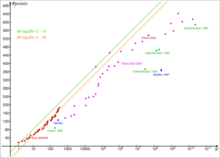
Figure 6. Curves with many points

The record so far for $\#C({\mathbb{Q}})/\log_{10}(2N+1)$ is held by the curve

$$y^{2}=37665x^{6}-220086x^{5}+212355x^{4}+268462x^{3}-209622x^{2}-69166x+49036$$

with $\#C({\mathbb{Q}})\geq 452$; the quotient is (at least) $78.88$.

7. Computations

Our data come from several sources.

7.1. Computations with (very) small curves

This began as a project whose aim it was to decide, for every genus 2 curve $C\in{\mathcal{C}}_{3}$, whether it possesses rational points. This experiment is described in [BS1], with more detailed explanation of the various methods used in [BS2, BS3, BS4].

These computations were later extended by the author. For those curves that do have rational points, we proceeded to find all rational points, or at least all rational points up to a height bound that is so large that we can safely assume that no larger points exist.

More precisely, the following was done. We determined a generating set for the Mordell-Weil group of the Jacobian of every curve (in a small number of cases, the rank is not yet proved to be correct: there is a difference of $2$ between the rank of the known subgroup and the 2-Selmer rank, which very likely comes from nontrivial elements of order 2 in the Shafarevich-Tate group). When the Mordell-Weil rank $r$ is zero, the set $C({\mathbb{Q}})$ of rational points on $C$ can be trivially determined. When $r=1$, a combination of Chabauty’s method and the Mordell-Weil sieve can be used to determine $C({\mathbb{Q}})$; this is described in [BS3]. For $r=2$, we can still use the Mordell-Weil sieve in order to find all points up to a height of $H=10^{1000}$ in reasonable time. For $r>2$, the sieving computation would take too long; in these cases, we have used a lattice point enumeration procedure on the Mordell-Weil group to find all points up to $H=10^{100}$. The following table summarizes what was done and gives the number of curves (up to isomorphism) for each value of the rank $r$. We denote the set of rational points on $C$ up to height $H$ by $C({\mathbb{Q}})_{H}$.

$r=0$	14 010 curves	$C({\mathbb{Q}})$ is determined.
$r=1$	46 575 curves	$C({\mathbb{Q}})$ is determined.
$r=2$	52 227 curves	$C({\mathbb{Q}})_{H}$ is determined for $H=10^{1000}$.
$r=3$	22 343 curves	$C({\mathbb{Q}})_{H}$ is determined for $H=10^{100}$.
$r=4$	2 318 curves	$C({\mathbb{Q}})_{H}$ is determined for $H=10^{100}$.
$r=5$	17 curves	$C({\mathbb{Q}})_{H}$ is determined for $H=10^{100}$.

Under the reasonable assumption that there are no points on these curves of height $>10^{100}$ (note that the largest point that we found has height about $2\cdot 10^{5}$), plus assuming that all the ranks are correct, this means that we have complete information on all rational points on curves in ${\mathcal{C}}_{3}$. We plan to extend our computations to ${\mathcal{C}}_{4}$ eventually.

7.2. All points with $H<2^{14}$ on curves with $N\leq 10$

Since $N=3$ is rather small, we also tried to get some information on somewhat larger curves. The author has written a program ratpoints (see [rp] for a description) that uses a quadratic sieve and fast bit-wise operations to search for rational points on hyperelliptic curves. On current hardware, it takes about 10 ms on average to find all points up to height $H=2^{14}-1=16383$ on a genus 2 curve.

We used up to 20 machines from the CLAMV teaching lab at Jacobs University Bremen for about one week in January 2008 to let ratpoints find all these points on all curves in ${\mathcal{C}}_{10}$. If $f\in{\mathbb{Z}}[x]$ is the polynomial defining the curve, then it is only necessary to look at one representative of the set

$$\{f(x),f(-x),x^{6}f(1/x),x^{6}f(-1/x)\}\,,$$

since the corresponding curves are isomorphic and the isomorphism preserves the height of the rational points. The total number of curves to be considered was therefore roughly $21^{7}/4\approx 450\cdot 10^{6}$, for a total of more than $100$ CPU days (the average time per curve on these machines was about 20 ms).

This gives us precise information on the frequency of points of height $<2^{14}$ on curves with $N\leq 10$. It also gives us close to complete information on curves with many points in this range, since curves with many points seem to have reasonably small points. We might have missed a few curves with (comparatively) many points that have one (or more?) additional point pair(s).

We plan to extend these computations to $N\leq 20$ (and possibly beyond), with the same height bound, once we have suitable hardware at our disposal.

7.3. Small curves with many points

To get some more data on curves with many points, we conducted a systematic search for curves in ${\mathcal{C}}_{50}$ with many points, making use of the observation that all curves in ${\mathcal{C}}_{10}$ that have comparatively many points tend to have points with $x$-coordinates $0$, $\infty$, $1$ and $-1$. Putting in the conditions that $F(0,1)$, $F(1,0)$, $F(1,1)$ and $F(-1,1)$ have to be squares reduces the search space to a sufficient extent so that a search up to $N=50$ is possible. The point search was first done with the bound $H=2^{10}-1=1023$; for those curves that had more than a certain number of points in this range, points were then counted up to height $H=2^{17}-1=131\,071$.

Based on the observation that all but one of the best curves that this computation revealed also have rational points at $x=\pm 2$ (maybe after a height-preserving isomorphism), we did a further systematic search for curves in ${\mathcal{C}}_{200}$ having rational points at all $x\in\{\infty,0,1,-1,2,-2\}$. Here the point search was done in three steps, using height bounds of $2^{12}-1=2047$, $2^{14}-1=16383$, and finally $2^{17}-1=131071$. Two threshold values for the number of points were used in order to decide whether to search for more points on a given curve.

We plan to extend these computations, too.

7.4. Curves with many points in Elkies’ families

Noam Elkies was so kind to provide us with explicit formulas for five ternary sextics $S(t,u,v)$ that admit many rational lines $\ell$ on which $S$ restricts to a perfect square. Setting the restriction of $S$ to a generic line equal to a square gives a curve of genus 2 that has a pair of rational points over each intersection point with a line $\ell$ as above. In this way, we obtain a 2-dimensional family of genus 2 curves with more than 50 pairs of rational points. We have conducted a systematic search among all lines $at+bu+cv=0$ with $a,b,c\in{\mathbb{Z}}$ and $\max\{|a|,|b|,|c|\}\leq 500$ in order to find curves with many points in these families.

There are two features of our computation that merit special mention. The first is that we used as a preliminary selection step a product $\prod_{p<X}\#C({\mathbb{F}}_{p})/p$ with $X=200$, which was required to be above a certain threshold value. The rationale behind this is that we expect a curve with many rational points also to have more ${\mathbb{F}}_{p}$-points than a random curve. Similar ideas have been used before. Note that each factor only depends on the reduction of the line $at+bu+cv=0$ mod $p$, so that we can precompute the relevant values and reduce the computation of the factors in the product to a table lookup.

The second is a systematic way of finding new rational points from known ones. If there are five rational points $(x_{i}/z_{i},y_{i}/z_{i}^{3})$ on a genus 2 curve $C$ that lie on a cubic $y=\alpha x^{3}+\beta x^{2}+\gamma x+\delta$, then the sixth intersection point of this cubic with $C$ is again a rational point. The condition is equivalent to the vanishing of the determinant of the matrix with rows $(z_{i}^{3},x_{i}z_{i}^{2},x_{i}^{2}z_{i},x_{i}^{3},y_{i})$. For reasons of efficiency, we have written a C program that first computes these determinants mod $2^{64}$ using native machine arithmetic; whenever a determinant appears to be zero, this is checked using exact arithmetic, and if the sixth intersection point is not yet known, it is recorded. We have applied this procedure to the points of height up to $10^{5}$ we found using ratpoints. This can produce quite a number of additional points of considerable height. For example, we were able to find eight more points on Stahlke’s curve from [Sta], so that this curve must have at least 374 rational points. Of course, in this way we can only find points within the subgroup of the Mordell-Weil group generated by the known points.

References

- [Bai] Stephan Baier, personal communication.
- [Beu] F. Beukers: The diophantine equation , Duke Math. J. 91, no. 1, 61–88 (1998).
- [BS1] N. Bruin and M. Stoll: Deciding existence of rational points on curves: an experiment, Experiment. Math. 17, 181–189 (2008).
- [BS2] N. Bruin and M. Stoll: 2-cover descent on hyperelliptic curves, to appear in Math. Comp.
- [BS3] N. Bruin and M. Stoll: The Mordell-Weil sieve: Proving non-existence of rational points on curves, in preparation.
- [BS4] N. Bruin and M. Stoll: Finding Mordell-Weil generators on genus 2 Jacobians, in preparation.
- [CHM] L. Caporaso, J. Harris and B. Mazur: Uniformity of rational points, J. Amer. Math. Soc. 10, 1–35 (1997).
- [DG] H. Darmon and A. Granville: On the equations and , Bull. London Math. Soc. 27, 513–543 (1995).
- [El1] N.D. Elkies: A parametrization of elliptic curves with a large integral point, at \hrefhttp://www.math.harvard.edu/ elkies/big_height.htmlhttp://www.math.harvard.edu/~elkies/big_height.html
- [El2] N.D. Elkies, personal communication.
- [Gra] A. Granville: Rational and integral points on quadratic twists of a given hyperelliptic curve, Internat. Math. Res. Notices 2007.8, Art. ID 027, 24 pp. (2007).
- [KK] W. Keller and L. Kulesz: Courbes algébriques de genre 2 et 3 possédant de nombreux points rationnels (French), C. R. Acad. Sci. Paris Sér. I Math. 321, 1469–1472 (1995).
- [Kul] L. Kulesz: Courbes algébriques de genre 2 possédant de nombreux points rationnels (French), C. R. Acad. Sci. Paris Sér. I Math. 321, 91–94 (1995).
- [PV] B. Poonen and J.F. Voloch: Random diophantine equations, in: Arithmetic of higher-dimensional algebraic varieties, B. Poonen and Yu. Tschinkel (eds.), Progress in Math. 226, pp. 175–184, Birkhäuser, 2004.
- [Sta] C. Stahlke: Algebraic curves over with many rational points and minimal automorphism group, Internat. Math. Res. Notices 1997, no. 1, 1–4 (1997).
- [Sto] M. Stoll: On the height constant for curves of genus two, II, Acta Arith. 104.2, 165–182 (2002)
-
[rp]
M. Stoll: Documentation for the ratpoints program,
Manuscript (2008).
arXiv:0803.3165v1 [math.NT]
ratpoints-2.0.1: \hrefhttp://www.mathe2.uni-bayreuth.de/stoll/programs/index.htmlhttp://www.mathe2.uni-bayreuth.de/stoll/programs/index.html