Protected Subspaces in Quantum Information

Abstract

In certain situations the state of a quantum system, after transmission through a quantum channel, can be perfectly restored. This can be done by “coding” the state space of the system before transmission into a “protected” part of a larger state space, and by applying a proper “decoding” map afterwards. By a version of the Heisenberg Principle, which we prove, such a protected space must be “dark” in the sense that no information leaks out during the transmission. We explain the role of the Knill-Laflamme condition in relation to protection and darkness, and we analyze several degrees of protection, whether related to error correction, or to state restauration after a measurement. Recent results on higher rank numerical ranges of operators are used to construct examples. In particular, dark spaces are constructed for any map of rank 2, for a biased permutations channel and for certain separable maps acting on multipartite systems. Furthermore, error correction subspaces are provided for a class of tri-unitary noise models.

I Introduction

We consider a quantum channel of finite dimension through which a quantum system in some state is sent. The output consists of another quantum state, and possibly some classical information. We are interested in the question to what extent the original quantum state can be recovered from that state and that information. In particular, we investigate if there are subspaces of the Hilbert space of the original system, on which the state can be perfectly restored.

In the literature a hierarchy of such spaces, which we shall call protected subspaces here, has been described. The strongest protection possible is provided in the case of a “decoherence free subspace” DG97 ; ZR97 ; LCW98a ; SL05 . In this case the channel acts on the subspace as a isometric transformation. All we have to do in order to recover the state, is to rotate it back.

The next strongest form of protection occurs when the channel acts on the subspace as a random choice between isometries, whose image spaces are mutually orthogonal. Then by measuring along a suitable partition of the output Hilbert space, it can be inferred from the output state which isometry has occurred, so that it can be rotated back. This situation is characterized by the well-known Knill–Laflamme criterion, BDSW96a ; KL97 and the protected subspace in this case is usually called an error correction subspace.

The weakest form of protection is provided in yet a third situation, which was encountered in the context of quantum trajectories and the purification tendency of states along these paths MK06 . In this case the deformation of the state is not caused by some given external device, but by the experimenter himself, who is performing a Kraus measurement Kr71 . Also in this case the “channel” acts as a random isometry, but the image spaces need not be orthogonal. It is now the measurement outcome (not the output state), that betrays to the experimenter which isometry has taken place. Using this information, he is able to undo the deformation of the component of the state that lies in the subspace considered.

It should be emphasized that the latter form of protection is far from a general error correction procedure. The experimenter only repairs the damage that he himself has incurred by his measurement.

Nevertheless, the above situations seem mathematically sufficiently similar to deserve study under a common title.

In all these three cases the experimenter learns nothing during the recovery operation about the component of the state inside our subspace. In this sense these subspaces can be considered “dark”, and this darkness is essential for the protection of information. Our main result (Theorem 3) is concerned with the equivalence between protection and darkness, which is a consequence of Heisenberg’s principle that no information on an unknown quantum state can be obtained without disturbing it (Corollary 2).

The question arises, for what channels protected subspaces are to be be found. We consider several examples in their Kraus decompositions. In each decomposition, we look for subspaces on which the channel acts as a multiple of an isometry, to be called a homometry here. Obviously, every (Kraus) operator $A$ acts homometrically on a one-dimensional space $\mathbbm{C}\psi$; its image $\mathbbm{C}A\psi$ is another one-dimensional space, and the shrinking factor is $\sqrt{\left\langle\,A\psi,A\psi\,\right\rangle}=\|A\psi\|$. However, one-dimensional spaces are useless as coding spaces for quantum states. What we shall need, therefore, is the recent theory of higher rank numerical ranges CKZ06b ; CKZ06 . With the help of this we shall be able to construct several examples.

The paper is organized as follows. A brief review of basic concepts including channels and instruments is presented in section II. We discuss Heisenberg’s principle in Section III. and prove our main Theorem, Theorem 3 in Section IV. In subsequent sections we analyze different forms of protected subspaces and compare their properties. In section V we review the notion of higher rank numerical range and quote some results on existence in the algebraic compression problem. Some examples of dark subspaces are presented in section VI, while an exemplary problem of finding an error correction code for a specific model of tri–unitary noise acting on a $3\times K$ system is solved in section VII.

II Channels and Instruments

Let $\mathcal{H}$ be a finite-dimensional complex Hilbert space, and let $\mathcal{B}(\mathcal{H})$ denote the space of all linear operators on $\mathcal{H}$. We consider $\mathcal{H}$ as the space of pure states of some quantum system. By a quantum operation or channel on this system we mean a completely positive map $\Phi:\mathcal{B}(\mathcal{H})\to\mathcal{B}(\mathcal{H})$ mapping the identity operator $\mathbbm{1}=\mathbbm{1}_{\mathcal{H}}$ to itself. The map $\Phi$ describes the operation “in the Heisenberg picture”, i.e. as an action on observables. Its description “in the Schrödinger picture”, i.e. as an action on density matrices $\rho$, is described by its adjoint $\Phi^{*}$. The maps $\Phi$ and $\Phi^{*}$ are related by

$$\forall_{\rho}\forall_{X\in\mathcal{B}(\mathcal{H})}:\quad\hbox{tr}\bigl{(}\Phi^{*}(\rho)X\bigr{)}=\hbox{tr}\bigl{(}\rho\Phi(X)\bigr{)}\;.$$

We note that the property $\Phi(\mathbbm{1})=\mathbbm{1}$, which we require for $\Phi$, is equivalent to trace preservation by $\Phi^{*}$:

$$\hbox{tr}\bigl{(}\Phi^{*}(\rho)\bigr{)}=\hbox{tr}\bigl{(}\Phi^{*}(\rho)\cdot\mathbbm{1}\bigr{)}=\hbox{tr}\bigl{(}\rho\cdot\Phi(\mathbbm{1})\bigr{)}=\hbox{tr}(\rho\cdot\mathbbm{1})=\hbox{tr}(\rho)\;.$$

By Stinespring’s theorem, every channel $\Phi:\mathcal{B}(\mathcal{H})\to\mathcal{B}(\mathcal{H})$ can be written as

$$\Phi(X)=V^{\dagger}(X\otimes\mathbbm{1}_{\mathcal{M}})V\;,$$ (1)

where $V$ is an isometry $\mathcal{H}\to\mathcal{H}\otimes\mathcal{M}$ for some auxiliary Hilbert space $\mathcal{M}$. The minimal dimension $r$ of $\mathcal{M}$ admitting such a representation is called the Choi rank Cho75a ; BZ06 of $\Phi$.

Any Stinespring representation of $\Phi$ naturally leads to a wider quantum operation

$$\Psi:\mathcal{B}(\mathcal{H})\otimes\mathcal{B}(\mathcal{M})\to\mathcal{B}(\mathcal{H}):X\otimes Y\mapsto V^{\dagger}(X\otimes Y)V\;,$$ (2)

which can be interpreted (in the Heisenberg picture) as the result of coupling the system to some ancilla having Hilbert space $\mathcal{M}$.

Thus Stinespring’s representation (1) can be symbolically rendered as in Fig. 1.

Figure 1: Stinespring’s dilation of $\Phi$ seen as coupling to an ancilla $\mathcal{M}$

In this picture, the cross stands for the substitution of $\mathbbm{1}_{\mathcal{M}}$ (in the Heisenberg picture, reading from right to left), or the partial trace (in the Schrödinger picture, reading from left to right). Physically, it corresponds to throwing away, or just ignoring, the ancilla after the interaction. In the picture, the fact that $\Psi$ is a compression, i.e. $\Psi=V^{\dagger}\cdot V$ for some isometry $V$, is symbolized by the triangular form of its box.

Now, by blocking the other exit in Fig. 1, we obtain the conjugate channel KNMR , $\Phi^{C}$:

$$\Phi^{C}:\mathcal{B}(\mathcal{M})\to\mathcal{B}(\mathcal{H}):\quad Y\mapsto\Psi(\mathbbm{1}_{\mathcal{H}}\otimes Y)=V^{\dagger}(\mathbbm{1}_{\mathcal{H}}\otimes Y)V\;.$$

See also Fig. 2.

Figure 2: The conjugate channel $\Phi^{C}$.

The main message of this paper is the following. The conjugate channel can be viewed as the flow of information into the environment. By Heisenberg’s Principle, to be explained below, such a flow prohibits the faithful transmission of information through the original channel $\Phi$. In particular, if the information encoded in some subspace of $\mathcal{H}$ is to be transmitted faithfully, nothing of it is visible from the outside: protection implies darkness. The degree of protection (decoherence free, strong or weak) is related to the degree of darkness, for which we shall define some terminology.

Any orthonormal basis $f=(f_{1},\ldots,f_{m})$ in $\mathcal{M}$ corresponds to a possible von Neumann measurement $\Pi_{f}^{*}$ on the ancilla, which maps a density matrix $\rho$ on $\mathcal{M}$ to a probability distribution $(\left\langle\,f_{1},\rho f_{1}\,\right\rangle,\left\langle\,f_{2},\rho f_{2}\,\right\rangle,\ldots,\left\langle\,f_{m},\rho f_{m}\,\right\rangle)$ on $\{1,2,\ldots,m\}$. (Cf. Fig. 3.) In the Heisenberg picture this is the map from the algebra $\mathbbm{C}^{m}$ with generators $e_{1}=(1,0,0,\ldots,0)$, $e_{2}=(0,1,0,\ldots,0)$, $\ldots$, $e_{m}=(0,0,\ldots,0,1)$, to $\mathcal{B}(\mathcal{M})$, given by

$$\Pi_{f}:\quad e_{i}\mapsto|f_{i}\rangle\langle f_{i}|\;.$$

Figure 3: Von Neumann measurement on $\mathcal{M}$.

In FIG. 3 the abelian algebra $\mathbbm{C}^{m}$ is indicated by a straight line since it only carries classical information. Quantum information is designated by a wavy line.

Let us now denote by $I_{f}$ the “partial inner product map”

$$\mathcal{H}\otimes\mathcal{M}\to\mathcal{H}:\quad\varphi\otimes\theta\mapsto\left\langle\,f,\theta\,\right\rangle\varphi\;,$$

and let us write

$$A_{i}:=I_{f_{i}}V\quad\in\mathcal{B}(\mathcal{H})\;.$$

Then since $I_{f_{i}}^{\dagger}XI_{f_{j}}=X\otimes|f_{i}\rangle\langle f_{j}|$, we obtain a decomposition of $\Phi$ along the basis $(f_{i})_{i=1}^{m}$ as follows:

$$\Phi(X)=\Psi(X\otimes\mathbbm{1}_{\mathcal{M}})=\sum_{i=1}^{m}\Psi\bigl{(}X\otimes|f_{i}\rangle\langle f_{i}|\bigr{)}=\sum_{i=1}^{m}V^{\dagger}I_{f_{i}}^{\dagger}XI_{f_{i}}V=\sum_{i=1}^{m}A_{j}^{\dagger}XA_{j}\;.$$ (3)

This is a Kraus decomposition of $\Phi$. Combining the coupling to the ancilla with a von Neumann measurement on the latter, we obtain an instrument in the language of Davies and Lewis DaL :

$$\Psi_{f}:\mathcal{B}(\mathcal{H})\otimes\mathbbm{C}^{m}\to\mathcal{B}(\mathcal{M}):\quad X\otimes e_{i}\mapsto V^{\dagger}(X\otimes|f_{i}\rangle\langle f_{i}|)V=A_{i}^{\dagger}XA_{i}\;.$$ (4)

The isometric property of $V$ is now expressed as

$$V^{\dagger}V=\sum_{i=1}^{m}A_{i}^{\dagger}A_{i}=\mathbbm{1}\;.$$ (5)

III Heisenberg’s Principle or Observer Effect

In quantum mechanics observables are represented as self-adjoint operators on a Hilbert space. When $A$ and $B$ are commuting operators, then they possess a common complete orthonormal set of eigenvectors. Each of these eigenvectors $\psi$ determines a state which associates sharply determined values to both observables $A$ and $B$.

But when $A$ and $B$ do not commute, such states may not exist. This important property of quantum mechanics was first discussed by Heisenberg Hei27 , and is called the Heisenberg Uncertainty Principle. It was formulated by Robertson Rob29 in the form

$$\sigma_{\psi}(A)\cdot\sigma_{\psi}(B)\geq\textstyle{{1\over 2}}|\left\langle\,\psi,(AB-BA)\psi\,\right\rangle|\;.$$

Here $\sigma_{\psi}(X)$ is the standard deviation of $X$ in the distribution induced by $\psi$. Already in the very same paper, Heisenberg introduced a second and very different principle, which is sometimes designated as the “Observer Effect”, and which we shall call the Heisenberg Principle here. Roughly speaking, it says that:

if $$A B$$ and do not commute, (6)

a measurement of $$B A$$ perturbs the probability distribution of . (7)

In the first half century of quantum mechanics, physicists, including Heisenberg himself, were satisfied with this formulation, and even considered it more or less identical to the Uncertainty Principle above.

In recent years it was realized that in fact we have here two different principles. Good quantitative formulations have been given of the Heisenberg Principle (for example Wer04 ; Jan06 ). For the purpose of the present paper we are satisfied with a qualitative (’yes-or-no’) version.

Let us first note that the formulation of the principle needs sharpening. As it stands, the condition is not needed: already in the trivial case that $A=B$ measurement of $B$ changes the probability distribution of $A$. Indeed changing the probability distribution of an observable is the very purpose of measurement! And also, when $A$ and $B$ commute, but are correlated, then gaining information on $B$ typically changes the distribution of $A$. A characteristic property of quantum theory only arises if we require that the outcome of the measurement of $A$ is not used in the determination of the new probability distribution of $B$. Even then, some states may go through unchanged.

Corrected for these observations, the Heisenberg Principle reads:

For noncommuting $$A B$$ and we cannot avoid that, (8)

for some initial states, a measurement of $$B A$$ changes the distribution of , (9)

even if we ignore the outcome of the measurement. (10)

The contraposition of the statement turns out to be mathematically more tractible:

If the probability distribution of $$A$$ is not altered in any initial state (11)

— by us performing some measurement and ignoring its outcome — (12)

then the object measured must commute with $$A$$. (13)

In this form it is sometimes called the ’nondemolition principle’.

Now let us make this statement precise. We start with a self-adjoint operator $A$ on $\mathcal{H}$. Its distribution in the state $\rho$ is determined by the numbers $\hbox{tr}(\rho g(A))$ when $g$ runs through the functions on the spectrum of $A$. Then some quantum operation is performed which on $\mathcal{B}(\mathcal{H})$ is described by a completely positive unit preserving map $\Phi$. We require that for all states $\rho$ and all functions $f$

$$\hbox{tr}\bigl{(}\Phi^{*}(\rho)g(A)\bigr{)}=\hbox{tr}\bigl{(}\rho g(A)\bigr{)}\;,$$

which is equivalent to

$$\Phi\bigl{(}g(A)\bigr{)}=g(A)\;.$$

I.e.: all elements of the *-algebra $\mathcal{A}$ consisting of functions of $A$ are left invariant by $\Phi$. Let us denote the commutant of $\mathcal{A}$ by $\mathcal{A}^{\prime}$,

$$\mathcal{A}^{\prime}=\{X\in\mathcal{B}(\mathcal{H})\,|\,\forall_{Y\in\mathcal{A}}\;:XY=YX\}\ .$$ (14)

Now, the quantum operation $\Phi$ is due to a measurement, so it is actually of the form

$$\Phi(X)=\Theta(X\otimes\mathbbm{1}),$$

where $\Theta:\mathcal{B}(\mathcal{H})\otimes\mathbbm{C}^{m}\to\mathcal{B}(\mathcal{H})$ is some instrument whose outcomes, labeled $1,2,\ldots,m$, in the state $\rho$ have probabilities $p_{1},p_{2},\ldots,p_{m}$ to occur, where

$$p_{j}=\hbox{tr}\bigl{(}\rho\Theta(\mathbbm{1}\otimes e_{j})\bigr{)}\;,$$

and where $\hbox{tr}\bigl{(}\rho\Theta(X\otimes e_{j})\bigr{)}/p_{j}$ is the expectation of $X$, conditioned on the outcome $j$. (This situation is comparable to, but more general than, that of $\Psi_{f}$ in (4).) Here $\mathbbm{C}^{m}$ is the algebra of measurement outcomes. Generalizing to arbitrary $\mathcal{A}$, we may now formulate the Heisenberg Principle as follows.

Proposition 1

(Heisenberg Principle.) Let $\mathcal{H}$ be a finite dimensional Hilbert space, and $\mathcal{B}$ some finite dimensional *-algebra. Let $\mathcal{A}$ be a sub-*-algebra of $\mathcal{B}(\mathcal{H})$, and let $\Theta$ be a completely positive unit preserving map $\mathcal{B}(\mathcal{H})\otimes\mathcal{B}\to\mathcal{B}(\mathcal{H})$. Suppose that for all $A\in\mathcal{A}$ we have

$$\Theta(A\otimes\mathbbm{1})=A\;.$$

Then for all $B\in\mathcal{B}$

$$\Theta(\mathbbm{1}\otimes B)\in\mathcal{A}^{\prime}\;.$$

Proof: For any density matrix $\rho$ on $\mathcal{H}$, define the quadratic form $D_{\rho}$ on $\mathcal{B}(\mathcal{H})\otimes\mathcal{B}$ by

$$D_{\rho}(X,Y):=\hbox{tr}\rho\bigl{(}\Theta(X^{*}Y)-\Theta(X)^{*}\Theta(Y)\bigr{)}\;.$$

By the Cauchy-Schwartz inequality for the completely positive map $\Theta$ this quadratic form is positive semidefinite. By assumption we have for all $A\in\mathcal{A}$:

$$D_{\rho}(A\otimes\mathbbm{1},A\otimes\mathbbm{1}) = \hbox{tr}\rho\bigl{(}\Theta(A^{*}A\otimes\mathbbm{1})-\Theta(A\otimes\mathbbm{1})^{*}\Theta(A\otimes\mathbbm{1})\bigr{)}$$

$$= \hbox{tr}\rho\bigl{(}A^{*}A\otimes\mathbbm{1}-(A\otimes\mathbbm{1})^{*}(A\otimes\mathbbm{1})\bigr{)}=0\;.$$

It then follows from the Cauchy-Schwartz inequality for $D_{\rho}$ itself that $D_{\rho}(A\otimes\mathbbm{1},\mathbbm{1}\otimes B)=0$ for all $B\in\mathcal{B}$. But then

$$\hbox{tr}\rho\bigl{(}A\Theta(\mathbbm{1}\otimes B)\bigr{)} = \hbox{tr}\rho\bigl{(}\Theta(A\otimes\mathbbm{1})\Theta(\mathbbm{1}\otimes B)\bigr{)}=\hbox{tr}\rho\bigl{(}\Theta\bigl{(}(A\otimes\mathbbm{1})(\mathbbm{1}\otimes B)\bigr{)}\bigr{)}=\hbox{tr}\rho\bigl{(}\Theta\bigl{(}(\mathbbm{1}\otimes B)(A\otimes\mathbbm{1})\bigr{)}\bigr{)}$$

$$= \hbox{tr}\rho\bigl{(}\Theta(\mathbbm{1}\otimes B)\Theta(A\otimes\mathbbm{1})\bigr{)}=\hbox{tr}\rho\bigl{(}\Theta(\mathbbm{1}\otimes B)A\bigr{)}.$$

Since this holds for all $\rho$, it follows that $\Theta(\mathbbm{1}\otimes B)$ commutes with $A$. $\square$

By taking $\mathcal{A}$ and $\mathcal{B}$ abelian, say $\mathcal{A}$ generated by some observable $A$, and $\mathcal{B}=\mathbbm{C}^{m}$ as above, and by choosing for $\Theta$ some instrument giving information about $B$, we obtain a statement of the type (13).

But there are other possible conclusions. We may choose $\mathcal{A}=\mathcal{B}(\mathcal{H})$, so that $\mathcal{A}^{\prime}=\mathbbm{C}\cdot\mathbbm{1}_{\mathcal{H}}$. Then the Heisenberg principle says that, if we wish to make sure that any possible state $\rho$ on $\mathcal{H}$ be unchanged by our measurement, no information at all concerning $\rho$ can be gained. This is expressed by the following corollary and FIG. 4.

Corollary 2

In the situation of Proposition 1, if for all $A\in\mathcal{B}(\mathcal{H})$ we have

$$\Theta(A\otimes\mathbbm{1})=A\;,$$

then there is a positive normalized linear form $\alpha$ on $\mathcal{B}$ such that for all $B\in\mathcal{B}$:

$$\Theta(\mathbbm{1}\otimes B)=\alpha(B)\cdot\mathbbm{1}_{\mathcal{H}}\;.$$

Indeed, the expectation of an outcome observable,

$$\hbox{tr}(\Theta^{*}\rho)(\mathbbm{1}\otimes B)=\hbox{tr}(\rho\Theta(\mathbbm{1}\otimes B))=\hbox{tr}(\rho\mathbbm{1}_{\mathcal{H}})\cdot\hbox{tr}(\alpha B)=\hbox{tr}(\alpha B)$$

does not depend on $\rho$ (see FIG. 4.)

Figure 4: Heisenberg’s Principle as an implication between diagrams

IV Protection and Darkness: the Knill-Laflamme Condition

Let $\mathcal{L}$ be a complex Hilbert space of dimension smaller than that of $\mathcal{H}$, and let $C:\mathcal{L}\to\mathcal{H}$ be some isometry. The range of $C$ is a subspace of $\mathcal{H}$, isomorphic with $\mathcal{L}$. Let $\Gamma:\mathcal{B}(\mathcal{H})\to\mathcal{B}(\mathcal{L})$ denote the compression map

$$\Gamma(X)=C^{\dagger}XC\;.$$

Note that $\Gamma$ is completely positive and identity-preserving. Compression maps are a convenient way of describing subspaces of a Hilbert space in the language of operations. Note that the operation $\Gamma^{*}$ (in the Schödinger picture) embeds density matrices on $\mathcal{L}$ into the range of $C$:

$$\Gamma^{*}(\rho)=C\rho C^{\dagger}\;.$$

Physically, $\Gamma$ is to be viewed as the “coding” operation.

Definition. We say that $\Gamma$ (or the subspace $C\mathcal{L}$ of $\mathcal{H}$) is protected against a channel $\Phi:\mathcal{B}(\mathcal{H})\to\mathcal{B}(\mathcal{H})$ if $\Gamma\circ\Phi$ is right-invertible, i.e. if there exists a “decoding” operation $\Delta:\mathcal{B}(\mathcal{L})\to\mathcal{B}(\mathcal{H})$ such that

$$\Gamma\circ\Phi\circ\Delta=\hbox{id}_{\mathcal{B}(\mathcal{L})}\;.$$ (15)

By virtue of (1) we may picture this state of affairs as in Fig. 5.

Figure 5: Strong protection of $\Gamma$ against $\Psi$

The subspace will be called weakly protected against an instrument $\Psi_{f}:\mathcal{B}(\mathcal{H})\otimes\mathbbm{C}^{m}\to\mathcal{B}(\mathcal{H})$ if $\Gamma\circ\Psi_{f}$ is right-invertible, i.e. if there exists a decoding operation $\Delta_{f}:\mathcal{B}(\mathcal{L})\to\mathcal{B}(\mathcal{H})\otimes\mathbbm{C}^{m}$ such that

$$\Gamma\circ\Psi_{f}\circ\Delta_{f}=\hbox{id}_{\mathcal{B}(\mathcal{L})}\;.$$ (16)

This is symbolically rendered in Fig. 6. The difference with Fig. 5 is that, in the case of weak protection, it is allowed to use the measurement outcome in the decoding. In the figure the classical information consisting of the measurement outcome, is symbolized by a straight line.

Figure 6: Weak protection of $\Gamma$ against $\Psi_{f}$

The above notions concern protection of information. Now we consider its availability to the external world.

Definition. Let $\Psi_{f}:\mathcal{B}(\mathcal{H})\otimes\mathbbm{C}^{m}\to\mathcal{B}(\mathcal{H})$ denote a quantum measurement (instrument) as described in (4). The subspace $C\mathcal{L}\subset\mathcal{H}$ (or the compression operation $\Gamma=C^{\dagger}\cdot C$), will be called dark with respect to $\Psi_{f}$ if for all $i=1,\ldots,m$ we have

$$\Gamma\circ\Psi_{f}(\mathbbm{1}\otimes e_{i})\in\mathbbm{C}\cdot\mathbbm{1}_{\mathcal{L}}\;.$$ (17)

This condition can be written in an equivalent form,

$$C^{\dagger}A_{i}^{\dagger}A_{i}C=\lambda_{i}\cdot\mathbbm{1}_{\mathcal{L}}{\rm\quad for\quad}i=1,\dots,m\;.$$ (18)

The subspace $C\mathcal{L}$ will be called completely dark for a channel $\Phi:\mathcal{B}(\mathcal{H})\to\mathcal{B}(\mathcal{H})$ if it is dark for all Kraus measurements $\Psi_{f}$ obtained by choosing different orthonormal bases in the ancilla space of some Stinespring dilation of $\Phi$; i.e.

$$\forall_{Y\in\mathcal{B}(\mathcal{M})}:\quad\Gamma\circ\Psi(\mathbbm{1}\otimes Y)\in\mathbbm{C}\cdot\mathbbm{1}_{\mathcal{L}}\;.$$ (19)

In terms of Kraus operators this is equivalent with the Knill-Laflamme condition:

$$C^{\dagger}A_{i}^{\dagger}A_{j}C=\alpha_{i,j}\cdot\mathbbm{1}_{\mathcal{L}}{\rm\quad for\quad}i,j=1,\dots,m\;.$$ (20)

Interpretation: From (17) and (18) we see that, if the von Neumann measurement along $f$ is performed, the measurement outcome $i$ has the same probability $\rho\bigl{(}\Gamma\circ\Psi_{f}(\mathbbm{1}\otimes e_{i})\bigr{)}=\rho(C^{\dagger}A_{i}^{\dagger}A_{i}C)=\lambda_{i}$, in all system states $\rho$, i.e. no information concerning the state $\rho$ can be read off from the $f$-measurement on the ancilla.

Complete darkness (i.e. (19) or the equivalent Knill-Laflamme condition (20)) says that no information whatsoever concerning the input state reaches the ancilla. Mathematically, the Knill-Laflamme condition says that the range of the conjugate channel lies entirely in the center $\mathbbm{C}\cdot\mathbbm{1}_{\mathcal{L}}$ of $\mathcal{B}(\mathcal{L})$. Let us emphasize again that if the space $C$ satisfies the conditions (20) for a map $\Psi$ represented by a particular set of the Kraus operators $\{A_{i}\}_{i=1}^{m}$, then $C$ also satisfies them for any other set of Kraus operators $\{B_{i}\}_{i=1}^{m^{\prime}}$, used to represent the same map $\Psi$.

Note also that the set of conditions (20), which express complete darkness, naturally defines a state $\alpha$, on the ancilla by a relation

$$\Gamma\circ\Psi(\mathbbm{1}\otimes Y)=\hbox{tr}(\alpha Y)\cdot\mathbbm{1}_{\mathcal{L}}\;.$$ (21)

satisfied by any $Y$. This quantum state acting on an auxiliary system is called the error correction matrix, since the density matrix $\alpha_{ij}$ appears in eq. (20). Observe that the density operator $\alpha$ depends only on the map $\Psi$ and not on the concrete form of the Kraus operators $A_{i}$, which represent the map and determine the matrix representation $\alpha_{ij}$ of $\alpha$. Relations between matrix elements of the same state represented in two different basis are governed by the Schrödinger lemma BZ06 , also called GHJW lemma Gi89 ; HJW93 .

We are now going to prove the equivalence of protection and darkness. In the case of strong protection and complete darkness this reproduces and puts into perspective the result of Knill and Laflamme KL97 In that case, if the state $\alpha$ is pure, then the decoding operation $\Delta$ can be realized by a unitary evolution, Hence the purity constraint for the error correction matrix, $\alpha=\alpha^{2}$, is the correct condition for a decoherence free subspace LBW99 – see also the proof of Theorem 3. As a quantitative measure, which characterizes to what extent a given protected space is close to a decoherence free space, one can use the von Neumann entropy of this state, $S=-{\rm Tr}\alpha\ln\alpha$. This code entropy KPZ08 is equal to zero if the protected space is decoherence free or if the information lost can be recovered by a reversible unitary operation. Observe that the code entropy $S$ characterizes the map $\Psi$ and the code space $C$, but does not depend on the particular Kraus form used to represent $\Psi$.

In this way we have determined a hierarchy in the set of protected spaces. Every decoherence free subspace belongs to the class of completely dark subspaces, which correspond to error correction codes. In turn the completely dark subspaces form a subset of the set of dark subspaces – see Fig. 7.

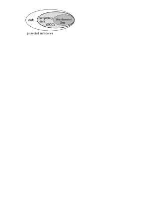
Figure 7: Sketch of the hierarchy of protected subspaces.

Theorem 3

(Equivalence of Protection and Darkness) Let $\mathcal{H}$, $\mathcal{M}$, and $\mathcal{L}$ be finite dimensional Hilbert spaces. Let $C:\mathcal{L}\to\mathcal{H}$ and $V:\mathcal{H}\to\mathcal{H}\otimes\mathcal{M}$ be isometries, and let $\Phi$, $\Psi$ and $\Psi_{f}$ be as defined in (1), (2) and (4). Then $C\mathcal{L}$ is weakly protected against the instrument $\Psi_{f}$ if and only if $C\mathcal{L}$ is dark for $\Psi_{f}$. It is strongly protected against $\Phi$ if and only if it is completely dark for $\Phi$.

Proof:

First assume that $C\mathcal{L}$ is strongly protected against $\Phi$, i.e. (15) holds for some decoding operation $\Delta$. Let $\Phi(X)=\Psi(X\otimes\mathbbm{1})$ for some compression $\Psi$. Define

$$\Theta:\mathcal{B}(\mathcal{L})\otimes\mathcal{B}(\mathcal{M})\to\mathcal{B}(\mathcal{L}):X\otimes Y\mapsto\Gamma\circ\Psi(\Delta(X)\otimes Y)\;.$$

Then $\Theta(X\otimes\mathbbm{1})=X$ for all $X\in\mathcal{B}(\mathcal{L})$, and by Corollary 2, since $\Delta(\mathbbm{1})=\mathbbm{1}$,

$$\Gamma\circ\Psi(\mathbbm{1}\otimes Y)=\Theta(\mathbbm{1}\otimes Y)\in\mathbbm{C}\cdot\mathbbm{1}\;.$$

so (19) holds, and $C\mathcal{L}$ is completely dark for $\Phi$.

Conversely, suppose that $C\mathcal{L}$ is completely dark for $\Psi$, and let $\alpha$ denote the density matrix given by (21) Then we may diagonalize:

$$\hbox{tr}(\alpha Y)=\sum_{i=1}^{m}a_{i}\left\langle\,f_{i},Yf_{i}\,\right\rangle$$

for some orthonormal set $(f_{i})_{i=1}^{m^{\prime}}$ (with $m^{\prime}\leq m$) of $\mathcal{B}(\mathcal{M})$ and positive numbers $a_{1},a_{2},\ldots,a_{m^{\prime}}$ summing up to 1. Now let $A_{i}:=I_{f_{i}}V$. Then for all $\psi\in\mathcal{L}$:

$$\left\langle\,A_{i}C\psi,A_{j}C\psi\,\right\rangle = \left\langle\,I_{f_{i}}VC\psi,I_{f_{j}}VC\psi\,\right\rangle$$

$$= \left\langle\,\psi,C^{\dagger}V^{\dagger}(\mathbbm{1}\otimes|f_{i}\rangle\langle f_{j}|)VC\psi\,\right\rangle$$

$$= \alpha(|f_{i}\rangle\langle f_{j}|)\cdot\|\psi\|^{2}$$

$$= a_{i}\delta_{ij}\cdot\|\psi\|^{2}\;.$$

So the ranges of $A_{i}C$ and $A_{j}C$ are orthogonal for $i\neq j$ and $A_{i}$ is homometric on $C\mathcal{L}$. Now define $D_{i}$ for $i=1,2,\ldots,m^{\prime}$ on these orthogonal ranges by

$$D_{i}\varphi=0\quad\hbox{if}\quad\varphi\perp\hbox{Range}\,(A_{i}C),\qquad D_{i}A_{i}C\psi=\sqrt{a_{i}}\psi\;.$$

($D_{i}$ “rotates back” the action of $A_{i}C$.) Let $\Delta$ denote the operation

$$\Delta(Z):=\sum_{i=1}^{m^{\prime}}D_{i}^{\dagger}ZD_{i}+\rho(Z)\left(\mathbbm{1}_{\mathcal{H}}-\sum_{j=1}^{m^{\prime}}D^{\dagger}D_{j}\right)\;.$$

for some arbitrary state $\rho$ on $\mathcal{B}(\mathcal{L})$. (The term with $\rho$ is intended to ensure that $\Delta(\mathbbm{1}_{\mathcal{L}})=\mathbbm{1}_{\mathcal{H}}$.) Then we have for all $Z\in\mathcal{B}(\mathcal{L})$:

$$\Gamma\circ\Phi\circ\Delta(Z) = \sum_{j=1}^{m^{\prime}}\sum_{i=1}^{m^{\prime}}C^{\dagger}A_{j}^{\dagger}D_{i}^{\dagger}ZD_{i}A_{j}C$$

$$= \sum_{j=1}^{m^{\prime}}\sum_{i=1}^{m^{\prime}}\frac{1}{a_{i}}C^{\dagger}A_{j}^{\dagger}A_{i}CZC^{\dagger}A_{i}^{\dagger}A_{j}C=\sum_{ij=1}^{m^{\prime}}\delta_{ij}a_{i}Z=Z\;.$$

So $C\mathcal{L}$ is strongly protected against $\Phi$ by (15).

Now let us prove the equivalence between weak protection and darkness. Assume that $C\mathcal{L}$ is weakly protected against $\Psi_{f}$, i.e. (16) holds for some $\Delta_{f}:\mathcal{B}(\mathcal{L})\to\mathcal{B}(\mathcal{H})\otimes\mathbbm{C}^{m}$, say $\Delta_{f}(X)=\sum_{j=1}^{m}\Delta^{j}_{f}(X)\otimes e_{j}$. Define $\Theta:\mathcal{B}(\mathcal{H})\otimes\mathbbm{C}^{m}\to\mathcal{B}(\mathcal{H})$ by

$$\Theta(X\otimes g):=\sum_{j=1}^{m}g(j)\Gamma\circ\Psi_{f}(\Delta^{j}(X)\otimes e_{j})\;.$$

Then by (16), $\Theta(X\otimes\mathbbm{1})=X$ for all $X\in\mathcal{B}(\mathcal{L})$. Hence by Corollary 2,

$$\Gamma\circ\Psi_{f}(\mathbbm{1}\otimes e_{i})=\Theta(\mathbbm{1}\otimes e_{i})\in\mathcal{B}(\mathcal{H})^{\prime}=\mathbbm{C}\cdot\mathbbm{1}_{\mathcal{L}}\;.$$

So (17) holds, and $C\mathcal{L}$ is dark for $\Psi_{f}$.

Conversely, assuming that $C\mathcal{L}$ is dark for $\Psi_{f}$, then $A_{l}C$ is homometric on $\mathcal{L}$ by (18), and we may define $D_{l}:\mathcal{H}\to\mathcal{L}$ by

$$D_{l}A_{l}C\psi:=\sqrt{\lambda_{l}}\psi\quad\hbox{if }\psi\in\mathcal{L},\qquad D_{l}\varphi=0\quad\hbox{ if }\varphi\perp\hbox{Range}\,(A_{l}C)\;.$$

(Briefly: $D_{l}=C^{\dagger}A_{l}^{\dagger}/\sqrt{\lambda_{l}}$ if $\lambda_{l}\neq 0$, zero otherwise.) Define the decoding operation $\Delta_{f}:\mathcal{B}(\mathcal{L})\to\mathcal{B}(\mathcal{H})\otimes\mathbbm{C}^{m}$ by

$$\Delta_{f}(Z):=\bigoplus_{l=1}^{m}\left(D_{l}^{\dagger}ZD_{l}+(\mathbbm{1}_{\mathcal{H}}-D_{l}^{\dagger}D_{l})\rho(Z)\right)$$

for some arbitrary state $\rho$ on $\mathcal{B}(\mathcal{L})$. Then, for $Z\in\mathcal{B}(\mathcal{L})$:

$$\Gamma\circ\Psi_{f}\circ\Delta_{f}(Z) = \Gamma\circ\Psi_{f}\left(\sum_{l=1}^{m}\bigl{(}D_{l}^{\dagger}ZD_{l}+(\mathbbm{1}-D_{l}^{\dagger}D_{l})\rho(Z)\bigr{)}\otimes e_{l}\right)$$

$$= C^{\dagger}V^{\dagger}\left(\sum_{l=1}^{m}\bigl{(}D_{l}^{\dagger}ZD_{l}+(\mathbbm{1}-D_{l}^{\dagger}D_{l})\rho(Z)\bigr{)}\otimes|f_{l}\rangle\langle f_{l}|\right)VC$$

$$= \sum_{l=1}^{m}C^{\dagger}A_{l}^{\dagger}D_{l}^{\dagger}ZD_{l}A_{l}C=\sum_{l=1}^{m}\frac{1}{\lambda_{l}}(C^{\dagger}A_{l}^{\dagger}A_{l}C)Z(C^{\dagger}A_{l}^{\dagger}A_{l}C)=\sum_{l=1}^{m}\lambda_{l}Z=Z\;.$$

$\square$

V Compression problems and generalized numerical range

For a given channel $\Phi:\mathcal{B}(\mathcal{H})\to\mathcal{B}(\mathcal{H})$ we are interested in the protected subspaces of $\mathcal{H}$. These are the subspaces on which the compressions of $A_{i}^{\dagger}A_{j}$ act as scalars. In this section we review this compression problem.

Let $T$ be an operator acting on a Hilbert space $\mathcal{H}$ of dimension $n$, say. For any $k\geq 1$, define the rank-$k$ numerical range of $T$ to be the subset of the complex plane given by

$$\Lambda_{k}(T)=\big{\{}\lambda\in{\mathbbm{C}}:C^{\dagger}TC=\lambda\mathbbm{1}\,\,{\rm for\,\,some\,\,}C:\mathbbm{C}^{k}\to\mathcal{H}\big{\}},$$ (22)

The elements of $\Lambda_{k}(T)$ can be called “compression-values” for $T$, as they are obtained through compressions of $T$ to a $k$-dimensional compression subspace. The case $k=1$ yields the standard numerical range for operators Bh97

$$\Lambda_{1}(T)=\{\langle\psi|{T\psi}\rangle\,:\,|\psi\rangle\in{\cal H}\,,\langle\psi|\psi\rangle=1\}.$$ (23)

It is clear that

$$\Lambda_{1}(T)\supseteq\Lambda_{2}(T)\supseteq\ldots\supseteq\Lambda_{n}(T).$$ (24)

The sets $\Lambda_{k}(T)$, $k>1$, are called higher-rank numerical ranges CKZ06b ; CHKZ07 . For any normal operator acting on ${\cal H}_{n}$ this is a compact subset of the complex plane. For unitary operators this set is included inside every convex hull $({\rm co}\,\Gamma)$, where $\Gamma$ is an arbitrary $(n+1-k)$-point subset (counting multiplicities) of the spectrum of $T$ CKZ06b . It was recently shown that for any normal operator the sets $\Lambda_{k}(T)$ are convex LS08 ; Wo08 while further properties of higher rank numerical range were investigated in CGHK08 ; LPS07 ; LPS07b .

The higher rank numerical range is easy to find for any Hermitian operator, $T=T^{\dagger}$ acting on an $n$-dimensional Hilbert space $\mathcal{H}$. Let us quote here a useful result proved in CKZ06b .

Lemma 4

Let $x_{1}\leq x_{2}\leq\dots\leq x_{n}$ denote the ordered spectrum (counting multiplicities) of a hermitian operator $T$. The rank-$k$ numerical range of $T$ is given by the interval

$$\Lambda_{k}(T)=[x_{k},x_{n+1-k}]\ ,$$ (25)

Note that the higher rank numerical range of a hermitian $T$ is nonempty for any $k\leq{\rm int}[(n+1)/2]$. Let us demonstrate an explicit construction of a compression to $\mathbbm{C}^{2}$ which solves equation (22) for a Hermitian matrix $T$ of size $n=4$. The latter’s eigenvalue equation reads $T|\phi_{i}\rangle=x_{i}|\phi_{i}\rangle$. Choose any real $\lambda\in\Lambda_{2}(T)=[x_{2},x_{3}]$. It may be represented as a convex combination of two pairs of eigenvalues $\{x_{1},x_{3}\}$ and $\{x_{2},x_{4}\}$ – see Fig. 8a. Writing

$$\lambda\ =\ (1-a)x_{1}+ax_{3}\ =\ (1-b)x_{2}+bx_{4}$$ (26)

one obtains the weights

$$a=\frac{\lambda-x_{1}}{x_{3}-x_{1}}=:\sin^{2}\theta_{1}{\rm\quad and\quad}b=\frac{\lambda-x_{2}}{x_{4}-x_{2}}=:\sin^{2}\theta_{2}$$ (27)

which determine real phases $\theta_{1}$ and $\theta_{2}$. These phases allow us to define an isometry $C:\mathbbm{C}^{2}\to\mathcal{H}$ by

$$C:\left\{\begin{array}[]{ccl}e_{1}&\mapsto&\cos\theta_{1}|\phi_{1}\rangle+\sin\theta_{1}|\phi_{3}\rangle\\ e_{2}&\mapsto&\cos\theta_{2}|\phi_{2}\rangle+\sin\theta_{2}|\phi_{4}\rangle\end{array}\right.,$$ (30)

Observe that

$$\left\langle\,e_{1},C^{\dagger}TCe_{1}\,\right\rangle=\cos\theta_{1}x_{1}\langle\phi_{1}|\psi_{1}\rangle+\sin\theta_{1}x_{3}\langle\phi_{3}|\psi_{1}\rangle=(1-a)x_{1}+ax_{3}=\lambda.$$ (31)

Similarly, we have $\left\langle\,e_{2},C^{\dagger}TCe_{2}\,\right\rangle=\lambda$. Further, we also have $\left\langle\,e_{1},C^{\dagger}TCe_{2}\,\right\rangle=0=\left\langle\,e_{2},C^{\dagger}TCe_{1}\,\right\rangle$. It follows that $C^{\dagger}TC=\mathbbm{1}$, and the isometry (30) provides a solution of the compression problem (22) as claimed. Note that one can select another pairing of eigenvalues, and the choice $\{x_{1},x_{4}\}$ and $\{x_{2},x_{3}\}$ allows us to get in this way another subspace $C^{\prime}\mathcal{L}$ spanned by vectors obtained by a superposition of states $|\phi_{1}\rangle$ with $|\phi_{4}\rangle$ and $|\phi_{2}\rangle$ with $|\phi_{3}\rangle$ respectively.

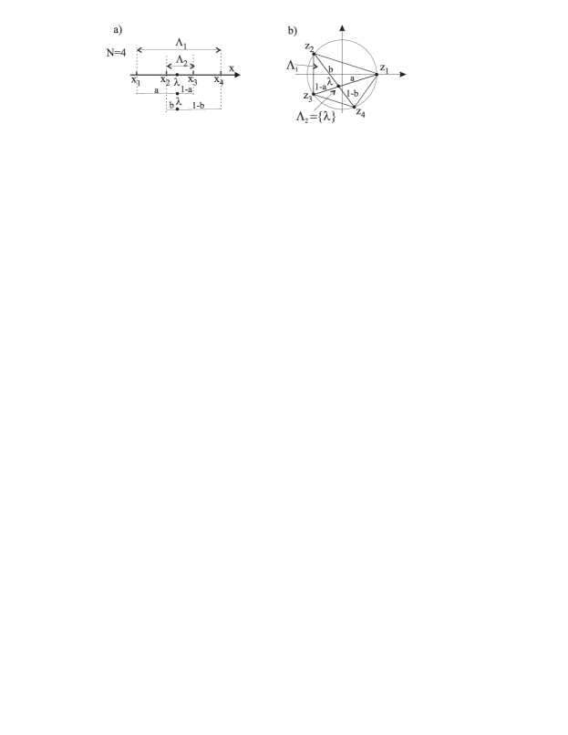
Figure 8: Standard numerical range $\Lambda_{1}$ and higher rank numerical range $\Lambda_{2}$ for a) Hermitian operator $T$ of size $4$ and b) non–degenerate unitary $U\in U(4)$. Observe similarity in finding the weights $a$ and $b$ used to construct superposition of states forming the subspace $C\mathcal{L}$ in both problems.

For a given operator $T$ one may try to solve its compression equation (22) and look for its numerical range $\Lambda_{k}(T)$. Alternatively, one may be interested in the following simple compression problem: For a given operator $T$ find all possible subspaces $C\mathcal{L}$ of a fixed size $k$ which satisfy (22).

Furthermore, it is natural to raise a more general, joint compression problem of order $M$. For a given set of $M$ operators $\{T_{1},\dots T_{M}\}$ acting on $\mathcal{H}_{n}$ find a subspace $C\mathcal{L}$ of dimensionality $k$ which solves simultaneously $M$ compression problems:

$$C^{\dagger}T_{m}C=\lambda_{m}\mathbbm{1}{\rm\quad for\quad}m=1,\dots,M\ .$$ (32)

Note that all compression constants, $\lambda_{m}\in\Lambda_{k}(T_{m})$, can be different, but the isometry $C$ needs to be the same.

VI Dark subspaces

In this section we provide several results concerning existence of darks spaces for several classes of quantum maps.

VI.1 Random external fields

Consider a noisy channel $\Phi$ given by

$$\Phi_{U}(X)=\sum_{i=1}^{r}q_{i}\,U_{i}^{\dagger}XU_{i},$$ (33)

where all operators $U_{i}$ are unitary while positive weights $q_{i}$ sum up to unity. Such maps are called random external fields AL87 or random unitary channels. The standard Kraus form (3) is obtained by setting $A_{i}=\sqrt{q_{i}}U_{i}$.

In this Kraus decomposition the whole space, and hence every subspace, is dark. This corresponds to the fact that the choice between the unitaries, which is made with the probability distribution $(q_{1},\ldots,q_{r})$, gives no information on the quantum state. And indeed, knowledge of the “external field”, i.e. of the outcome $i$, permits us to undo, by the inverse of $U_{i}$, the action of the channel.

VI.2 Rank two quantum channels

Let us now analyze a rank two channel,

$$\rho^{\prime}=\Phi_{2}(\rho)=A_{1}\rho A_{1}^{\dagger}+A_{2}\rho A_{2}^{\dagger}\ ,$$ (34)

Lemma 5

For any Kraus representation of any rank-two channel acting on a system of size $N$ there exist a dark subspace of dimension $k={\rm int}[(N+1)/2].$

Proof. We need to solve a joint compression problem (32) of order two, for two Hermitian operators $T_{1}=A_{1}^{\dagger}A_{1}$ and $T_{2}=A_{2}^{\dagger}A_{2}$. Due to Lemma 4 there exists a subspace $P_{k}$ of dimension $k={\rm int}[(N+1)/2]$ which solves the compression problem for the Hermitian operator $T_{1}$ of size $N$. It is also a solution of the compression problem for the other operator, since the trace preserving condition implies $T_{2}={\mathbbm{1}}-T_{1}$. $\square$

VI.3 Biased permutation channel

Consider a quantum map acting on a system of arbitrary size $n$ described by the Kraus form (3). Let us assume that all Kraus operators are given by ’biased permutations’

$$A_{i}=P_{i}\sqrt{D_{i}}\ ,\quad i=1,\dots,r\ .$$ (35)

where $D_{i}$ is a diagonal matrix containing non-negative entries, and $P_{i}$ denotes an arbitrary permutation of the $N$-element set. Hence all elements of the POVM form diagonal matrices,

$$T_{i}=A_{i}^{\dagger}A_{i}=\sqrt{D_{i}}P_{i}^{\dagger}P_{i}\sqrt{D_{i}}=D_{i}\ ,$$ (36)

in general not proportional to identity. Note that the Kraus operators defined in this way need not to be Hermitian. To satisfy the trace preserving condition (5) we need to assume that $\sum_{i=1}^{r}D_{i}={\mathbbm{1}}$. Let us define an auxiliary rectangular matrix of size $r\times N$, namely $S_{im}:=(D_{i})_{mm}\geq 0$. Then the above constraints for the matrices $D_{i}$ is equivalent to the statement that $S$ is stochastic, since the sum of all elements in each column is equal to 1,

$$\sum_{i=1}^{r}S_{im}=1{\rm\quad for\quad}m=1,\dots,N\ .$$ (37)

A map described by Kraus operators fulfilling relations (35) and (37) will be called a biased permutation channel.

We are going to construct a dark space for a wide class of such channels. For simplicity assume that the size of the system is even, $N=2k$. Let us additionally assume that all elements in each row of $B$ are ordered (increasingly or decreasingly) and that the matrix $S$ enjoys a symmetry relation,

$$S_{i,m}+S_{i,n-m+1}={\rm const}=:\lambda_{i}{\rm\quad for\quad}i=1,\dots,r;\quad m=1,\dots,k=n/2\ .$$ (38)

Then the numbers $\lambda_{i}$ can be defined by a sum of the entries in each row, $\lambda_{i}=\frac{2}{N}\sum_{m=1}^{N}S_{im}$.

Lemma 6

Assume that a biased permutation channel acting on a system of size $N=2k$ possesses the symmetry relation (38). Then it has a dark space of dimension $k=n/2$.

Proof. We need to find a joint compression subspace for the set of $r$ elements of POVM given by diagonal matrices $D_{i}$, with $i=1,\dots,r$. Since these matrices commute, they have the same set of eigenvectors, denoted by $|v_{m}\rangle$, $m=1,\dots,N$. Due to symmetry relation (38) we know that the barycenter of each spectrum, $\lambda_{i}$ belongs to the higher rank numerical range, $\Lambda_{k}(D_{i})$. Furthermore, this relation shows that (for any $i$) the number $\lambda_{i}$ can be represented as a sum of two eigenvalues of $D_{i}$ with the same weights, $\lambda_{i}=\frac{1}{2}(D_{i})_{mm}+\frac{1}{2}(D_{i})_{m^{\prime}m^{\prime}}$ with $m^{\prime}=n+1-m$. By construction this property holds for all operators $D_{i}$, $i=1,\dots r$. Hence the general construction of the higher order numerical range for Hermitian operators CKZ06 implies that the subspace

$$C_{k}:=\sum_{i=1}^{k}|\psi_{i}\rangle\langle\psi_{i}|{\rm\quad where\quad}|\psi_{i}\rangle:=\frac{1}{\sqrt{2}}(|v_{i}\rangle+|v_{1-i+N}\rangle)$$ (39)

fulfills the joint compression problem for all operators $T_{i}=D_{i}$, $i=1,\dots r$. Hence this subspace is dark as advertised. $\square$

To watch the above construction in action consider a three biased permutation channel acting on a two qubit system. Hence we set $r=3$ and $N=4$, and assume that five real weights satisfy $0<a<b<x/2<1/2$ and $0<c<d<x/2$. They can be used to define the channel by a stochastic matrix $S$

$$S=\begin{pmatrix}a&b&x-b&x-a\\ c&d&x-d&x-c\\ a^{\prime}&b^{\prime}&b^{\prime\prime}&a^{\prime\prime}\\ \end{pmatrix}\ ,$$ (40)

where $a^{\prime}=1-a-c$, $b^{\prime}=1-b-d$, $a^{\prime\prime}=1-2x+a+c$ and $b^{\prime\prime}=1-2x+b+d$. Note that this matrix satisfies the symmetry condition (38), the elements in each row are ordered, while mean weights in each row read $\lambda_{1}=\lambda_{2}=x/2$ and $\lambda_{3}=2(1-x)$.

To complete the definition of the channel we need to specify three permutation matrice of size four. For instance let us choose $P_{1}=P_{(1,2,3,4)}$, $P_{2}=P_{(1,2),(3,4)}$ and $P_{3}=P_{(1,4,3,2)}$, where according to the standard notion, the subscripts contain the permutation cycles. Then the biased permutation channel is defined by the three Kraus operators

$$A_{1}=\begin{pmatrix}0&\sqrt{b}&0&0\\ 0&0&\sqrt{x-b}&0\\ 0&0&0&\sqrt{x-a}\\ \sqrt{a}&0&0&0\\ \end{pmatrix}\ ,\ A_{2}=\begin{pmatrix}0&\sqrt{d}&0&0\\ \sqrt{c}&0&0&0\\ 0&0&0&\sqrt{x-c}\\ 0&0&\sqrt{x-d}&0\\ \end{pmatrix}\ ,\ A_{3}=\begin{pmatrix}0&0&0&\sqrt{a^{\prime\prime}}\\ \sqrt{a^{\prime}}&0&0&0\\ 0&\sqrt{b^{\prime}}&0&0\\ 0&0&\sqrt{b^{\prime\prime}}&0\\ \end{pmatrix}\ ,$$ (41)

which satisfy the trace preserving condition (5).

Since the barycenter $\lambda_{i}$ of the spectrum of the POVM element $T_{i}=D_{i}$ (given by a row of matrix (40)), is placed symmetrically, in all three cases it can be represented by a convex combination of pairs of eigenvalues with weights equal to $1/2$. Thus we define two pure states

$$|\psi_{1}\rangle:=\frac{1}{\sqrt{2}}(|v_{1}\rangle+|v_{4}\rangle)\ ,\quad|\psi_{2}\rangle:=\frac{1}{\sqrt{2}}(|v_{2}\rangle+|v_{3}\rangle)\ ,$$ (42)

and the two dimensional subspace spanned by them, $C=|\psi_{1}\rangle\langle\psi_{1}|+|\psi_{2}\rangle\langle\psi_{2}|$. It is easy to verify that the subspace $C$ satisfies $C^{\dagger}T_{1}C=\lambda_{1}\mathbbm{1}=C^{\dagger}T_{2}C$ while $C^{\dagger}T_{3}C=\lambda_{3}\mathbbm{1}$ so this space is dark. Note that the subspace $C\mathcal{L}$ cannot be used to design an error correcting code since $C^{\dagger}A_{1}^{\dagger}A_{2}C\notin\mathbbm{C}\cdot\mathbbm{1}$.

VI.4 Composed systems and separable channels

Consider a bipartite system of size $n=n_{A}\times n_{B}$. A quantum operation $\Phi$ acting on this bipartite system is called local, if it has a tensor product structure, $\Phi=\Phi_{A}\otimes\Phi_{B}$, where both maps $\Phi_{A}$ and $\Phi_{B}$ are completely positive and preserve the identity. If for both individual operations, $\Phi_{A}$ and $\Phi_{B}$, there exist protected subspaces $C_{k}$ and $Q_{l}$ respectively, then the product subspace $C_{k}\otimes Q_{l}$ of size $kl$ is also a protected subspace for the composite map $\Phi_{A}\otimes\Phi_{B}$.

Similar protected subspaces of the product form can be constructed for a wider class of separable maps (see e.g. BZ06 ),

$$\rho^{\prime}=\Phi^{*}(\rho)=\sum_{i=1}^{r}(A_{i}\otimes B_{i})\rho(A_{i}\otimes B_{i})^{\dagger}.$$ (43)

Assume that a subspace $C_{k}\in{\cal H}_{N_{A}}$ is a solution of the joint compression problem for the set of $r$ operators $A_{i}^{\dagger}A_{i}$, while a subspace $Q_{l}\in{\cal H}_{N_{B}}$ does the job for the set of $r$ operators $B_{i}^{\dagger}B_{i}$. It is then easy to see that the product subspace $C_{k}\otimes Q_{l}$ of dimension $kl$ is a dark subspace for the separable map (43).

It is straightforward to extend lemmas 3 and 4 for separable maps acting on composite systems and apply them to construct protected subspaces with a product structure. On the other hand, if for certain problems such product code subspace do not exist, one may still find a code subspace spanned by entangled states. Such a problem for the tri–unitary model is solved in following section.

VII Unitary noise and error correction codes

In this section we are going to study multiunitary noise (33), also called random external fields, and look for existence of error correction codes, i.e. completely protected subspaces. In general the number $r$ of unitary operators defining the channel can be arbitrary but we will restrict our attention to the cases in which this number is small.

VII.1 Bi–unitary noise model

The case in which $r=2$, referred to as bi-unitary noise was recently analyzed in CKZ06 ; CHKZ07 . Let us rewrite the dynamics in the form

$$\rho^{\prime}=\Phi^{*}(\rho)=qV_{1}^{\rho}V_{1}^{\dagger}+(1-q)V_{2}\rho V_{2}^{\dagger}\ .$$ (44)

and assume that we deal with the system of two qubits. Then both unitary matrices $V_{1}$ and $V_{2}$ belong to $U(4)$ while probability $p$ belongs to $[0,1]$. The problem of finding the compression $C$ for the above map is shown to be equivalent to the case

$$\rho^{\prime\prime}=\Phi^{*}(\rho)=q\rho+(1-q)U\rho U^{\dagger}$$ (45)

where $U=V_{1}^{\dagger}V_{2}$.

Thus the error correction matrix $\alpha$ of size two defined by eq. (21) reads

$$\alpha\ =\ \left(\begin{matrix}q&\sqrt{q(1-q)}\lambda\\ \sqrt{q(1-q)}\lambda^{*}&1-q\end{matrix}\right)$$ (46)

where $\lambda$ is solution of the compression problem for $U$

$$C^{\dagger}UC=\lambda\cdot\mathbbm{1}\ .$$ (47)

Thus to find the error correction space for the bi–unitary model it is sufficient to solve the compression equation for a single operator $U$. A solution exists for any unitary $U$ CKZ06 , but for simplicity we will consider here the generic case if the spectrum of $U$ is not degenerated. Assume that the phases these unimodular numbers $z_{1},...,z_{4}$ are ordered and that $|\psi_{i}\rangle$ denote the corresponding eigenvectors.

Let $\lambda$ denote the intersection point between two chords of the unit circle, $z_{1}z_{3}$ and $z_{2}z_{4}$; compare Fig. 8b. This point can be represented as a convex combination of each pair of complex eigenvalues,

$$\lambda\ =\ (1-a)z_{1}+az_{3}\ =\ (1-b)z_{2}+bz_{4}\ ,$$ (48)

where the non–negative weights read

$$a=\frac{\lambda-z_{1}}{z_{3}-z_{1}}=:\sin^{2}\theta_{1}{\rm\quad and\quad}b=\frac{\lambda-z_{2}}{z_{4}-z_{2}}=:\sin^{2}\theta_{2}$$ (49)

and determine real phases $\theta_{1}$ and $\theta_{2}$. Note similarity with respect to the construction used in the Hermitian case, in which (26) represents a convex combination of points on the real axis. In an analogy with the reasoning performed for a hermitian $T$ we define according to (30) an orthonormal pair of vectors $|\psi_{1}\rangle$ and $|\psi_{2}\rangle$ and define the associated isometry $C:e_{j}\mapsto\psi_{j}$. Since $\langle U\psi_{1}|\psi_{1}\rangle=\lambda=\langle U\psi_{2}|\psi_{2}\rangle$ and $\langle U\psi_{1}|\psi_{2}\rangle=0=\langle U\psi_{2}|\psi_{1}\rangle$ then $CUC=\lambda{\mathbbm{1}}$. Therefore $\lambda$ belongs to $\Lambda_{2}(U)$ as claimed and the range of $C$ provides the error correction code for the bi-unitray noise (45) acting on a two-qubit system.

In the case of doubly degenerated spectrum of $U$ the complex number $\lambda$ is equal to the degenerated eigenvalue, so its radius, $|\lambda|$, is equal to unity. In this case the matrix $\alpha$ given in (20) represents a pure state, $\alpha=\alpha^{2}$, so the two–dimensional subspace spanned by both eigenvectors corresponding to the degenerated eigenvalues is decoherence free.

Bi–unitary noise model for higher dimensional systems was analyzed in CHKZ07 . It was shown in this work that for a generic $U$ of size $N$ there exists a code subspace of dimensionality $k={\rm int}[(N+2)/3]$. This result implies that for a system of $m$ qubits and a generic $U$ of size $N=2^{m}$ there exists an error correction code supported on $m-2$ qubits. Furthermore, if $N=d^{m}$ and $d\geq 3$, there exists a code supported on $m-1$ quantum systems of size $d$.

VII.2 Tri–unitary noise model

Consider now a model of noise described by three unitary operations acting on a bipartite, $N=2\times N_{B}$ system,

$$\rho^{\prime}=\Phi^{*}(\rho)=q_{1}V_{1}\rho V_{1}^{\dagger}+q_{2}V_{2}\rho W_{2}^{\dagger}+(1-q_{1}-q_{2})V_{3}\rho V_{3}^{\dagger}\ .$$ (50)

Performing a unitary rotation in analogy to (45) we obtain an equivalent form

$$\rho^{\prime\prime}=\Phi^{*}(\rho)=q_{1}\rho+q_{2}U_{1}\rho U_{1}^{\dagger}+(1-q_{1}-q_{2})U_{2}\rho U_{2}^{\dagger}\ .$$ (51)

The model is thus characterized by two unitary matrices of size $N$, namely $U_{1}=V_{1}^{\dagger}V_{2}$ and $U_{2}=V_{1}^{\dagger}V_{3}$. and two weights $q_{1}$ and $q_{2}$, which we assume to be positive with their sum smaller than unity.

To find a simplest error correction code for this model one needs to find a two-dimensional subspace, which forms a joint solution of three compression problems

$$\left\{\begin{array}[]{ccc}C^{\dagger}U_{1}C&=&\lambda_{U_{1}}\mathbbm{1}\\ C^{\dagger}U_{2}C&=&\lambda_{U_{2}}\mathbbm{1}\\ C^{\dagger}WC&=&\lambda_{W}\mathbbm{1}\\ \end{array}\right.,$$ (52)

where $W=U_{1}^{\dagger}U_{2}$. Each of the above three problems may be solved using the notion of the higher rank numerical range of a unitary matrix. However, for generic unitary matrices $U_{1}$ and $U_{2}$ of size $4$ the corresponding compression subspaces do differ. Thus for a typical choice of the unitary matrices the tri–unitary noise model will not have an error correction code, for which it is required that the subspace $C$ solves all three problems simultaneously.

There exist several examples of two commuting matrices $U_{1}$ and $U_{2}$ of size $N=4$, such that they possess the same solution $C$ of the compression problem. However, to assure that it coincides with the solution of the same problem for $W=U_{1}^{\dagger}U_{2}$, we will analyze an exemplary system of size $n=2\times 3$. Consider two unitary matrices of a tensor product form,

$$\left\{\begin{array}[]{ccc}U_{1}&=&U_{A}^{\dagger}\otimes U_{B}\\ U_{2}&=&U_{A}\otimes U_{B}\end{array}\right.$$ (53)

where

$$U_{A}=\left(\begin{array}[]{ccc}1&0&0\\ 0&e^{-i\alpha}&0\\ 0&0&e^{i\alpha}\end{array}\right){\quad\rm and\quad}U_{B}=\left(\begin{array}[]{cc}1&0\\ 0&e^{i\xi}\end{array}\right)\ .$$ (54)

Observe that $U_{1}$ and $U_{2}$ do commute, so they share the same set of eigenvectors. Assume that the phases satisfy $\alpha\in(\pi/2,\pi)$ and $\xi\in\bigl{(}0,{\rm min}\{\alpha,2(\pi-\alpha)\}\bigr{)}$. Then the ordered spectra of both matrices read

$$U_{1}={\rm diag}\Big{\{}1,e^{i\xi},e^{i\alpha},e^{i(\alpha+\xi)},e^{-i\alpha},e^{i(\xi-\alpha)}\Big{\}},{\quad\quad}U_{2}={\rm diag}\Big{\{}1,e^{i\xi},e^{-i\alpha},e^{i(\xi-\alpha)},e^{i\alpha},e^{i(\alpha+\xi)}\Big{\}},$$ (55)

and differ only by the order of the eigenvalues. Both unitary matrices are represented in Fig. 9 in which $z_{i}$, $i=1,\dots,6$ denote the ordered eigenvalues of $U_{1}$ while $|\varphi_{i}\rangle,i=1,\ldots,6$ are eigenvectors of this matrix. The same states form also the set of eigenvectors of $U_{2}$, but they correspond to other eigenvalues. Let $z_{i}^{\prime}$ denote the ordered eigenvalues of $U_{2}$. Then $|\varphi_{3}\rangle$ corresponds to $z_{3}^{\prime}=z_{5}$ while $|\varphi_{5}\rangle$ corresponds to $z_{5}^{\prime}=z_{3}$.

The third of the unitaries also has also a tensor product form,

$$W=U_{1}^{\dagger}U_{2}=(U_{A}^{\dagger}\otimes U_{B})^{\dagger}(U_{A}\otimes U_{B})=U_{A}^{2}\otimes\mathbbm{1}_{2}.$$ (56)

Hence the spectrum of $W$, denoted by $z_{i}^{\prime\prime}$, consists of three pairs of doubly degenerated eigenvalues, $W={\rm diag}\Big{\{}1,1,e^{-2i\alpha},e^{-2i\alpha},e^{2i\alpha},e^{2i\alpha}\Big{\}}$, see Fig. 10.

Numerical range of rank two for matrices $U_{1}$, $U_{2}$ and $W$ is shown in the pictured as a gray region. Each point $\lambda\in\Lambda_{2}(U_{1})$ offers a subspace $C_{2}$ which forms a solution of the first of three equations (52). However, the other two equations restrict further constraints for $\lambda$.

To construct an error correction code for the tri-unitary noise model we are going to follow the strategy used above for solving the compression problem: we split the Hilbert space into a direct sum of two subspaces of size three, and try to construct a single state in each subspace. More formally we define the subspace

$$C_{2}=\sum_{i=1}^{2}|\psi_{i}\rangle\langle\psi_{i}|$$ (57)

where each state is obtained by a coherent superposition of three eigenstates of $U_{1}$,

$$\left\{\begin{array}[]{ccc}|\psi_{1}\rangle&=&\sqrt{a_{1}}|\varphi_{1}\rangle+\sqrt{a_{3}}|\varphi_{3}\rangle+\sqrt{a_{5}}|\varphi_{5}\rangle\\ |\psi_{2}\rangle&=&\sqrt{a_{2}}|\varphi_{2}\rangle+\sqrt{a_{4}}|\varphi_{4}\rangle+\sqrt{a_{6}}|\varphi_{6}\rangle\end{array}\right..$$ (58)

Since the unitary operators $U_{i}$ can be expressed as tensor product of diagonal matrices (e.g. $U_{2}=U_{A}\otimes U_{B}$), their joint set of eigenvectors consits of product pure states only. On the other hand, the states $|\psi_{1}\rangle$ and $|\psi_{2}\rangle$ are by construction entangled.

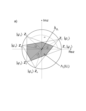
Figure 9: Numerical range (gray space): a) $\Lambda_{2}(U_{1})$; b) $\Lambda_{2}(U_{2})$

The weights $a_{1}$ are defined as a weights obtained by representing point $\lambda$ by a convex combination of the triples of eigenvalues. Since we wish to get a space $C$ being a joint solution of all three equations (52), we are going to require that the same weights $a_{i}$ can be used to form the compression value $\lambda$ as a combination of both triples of eigenvalues for each spectrum,

$$\left\{\begin{array}[]{ccccc}\lambda_{U_{1}}&=&a_{1}z_{1}+a_{3}z_{3}+a_{5}z_{5}&=&a_{2}z_{2}+a_{4}z_{4}+a_{6}z_{6}\\ \lambda_{U_{2}}&=&a_{1}z^{\prime}_{1}+a_{3}z^{\prime}_{3}+a_{5}z^{\prime}_{5}&=&a_{2}z^{\prime}_{2}+a_{4}z^{\prime}_{4}+a_{6}z^{\prime}_{6}\\ \lambda_{W}&=&a_{1}z^{\prime\prime}_{1}+a_{3}z^{\prime\prime}_{3}+a_{5}z^{\prime\prime}_{5}&=&a_{2}z^{\prime\prime}_{2}+a_{4}z^{\prime\prime}_{4}+a_{6}z^{\prime\prime}_{6}\end{array}\right.$$ (59)

where $z_{i}$, $z_{i}^{\prime}$ and $z_{i}^{\prime\prime}$ denote ordered spectra of $U_{1}$, $U_{2}$ and $W$, respectively. It is now clear that for a generic choice of $U_{1}$ and $U_{2}$ (which implies $W=U_{1}^{\dagger}U_{2}$), such a system has no solutions. However, if both diagonal matrices are of the special form (55), there exists a solution of the problem. The weights $a_{i}$ satisfy

$$\left\{\begin{array}[]{ccccc}a_{1}&=&a_{2}&=&1+\displaystyle\frac{1}{-1+\cos\alpha}\\ \\ a_{3}&=&a_{4}&=&\displaystyle\frac{1}{2-2\cos\alpha}\\ \\ a_{5}&=&a_{6}&=&\displaystyle\frac{1}{2-2\cos\alpha}\end{array}\right.$$ (60)

and imply the following compression values

$$\left\{\begin{array}[]{ccc}\lambda_{U_{1}}&=&0\\ \lambda_{U_{2}}&=&0\\ \lambda_{W}&=&-1-2\cos\alpha\end{array}\right..$$ (61)

Due to the symmetry of the problem the latter number $\lambda_{W}$ is real.

Substituting the weights (60) into (58) we get an explicit form (57) of the subspace $C$. It is now easy to check that this subspace satisfies simultaneously all three equations (52) with compression values given by (61), hence it provides a two dimensional error correction code for this noise model. This solution is correct for any unitaries $U_{1}$ and $U_{2}$ having any set of eigenvectors $|\varphi_{i}\rangle,\ i=1,\ldots,6$ and spectra given by (55) and parameterized by phases $\alpha$ and $\xi$.

The above construction can be generalized for a tri–unitary noise model acting on larger system of size $N=3\times K$ Ma07 . An error correction code of size $K$ exists in this case, if matrices $U_{1}$ and $U_{2}$ have the tensor product form (53), where $U_{A}={\rm diag}\Big{\{}1,e^{i\alpha},e^{-i\alpha}\Big{\}}$ as before and $U_{B}={\rm diag}\Big{\{}1,e^{i\xi_{2}},e^{i\xi_{3}},\dots,e^{i\xi_{K}}\Big{\}}$. The code subspace $C=\sum_{i=1}^{K}|\psi_{i}\rangle\langle\psi_{i}|$ is then obtained in an analogous way, by representing the Hilbert space as a direct product of $K$ subspaces of dimension three each and constructing each state $|\psi_{i}\rangle$ as a coherent superposition of three eigenstates of $U_{1}$ corresponding to a triple of eigenvalues $z_{l},z_{l+K}$ and $z_{l+2K}$ for $l=1,\dots K$. Note that the code space constructed here for the bipartite system does not have the tensor product structure, since it is spanned by entangled states (58).

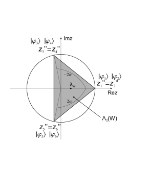
Figure 10: Numerical range $\Lambda_{2}(W)$ is represented by a dark triangle

VIII Conclusions

This paper concerns finite dimensional instruments or Kraus measurements, acting on a quantum system with Hilbert space $\mathcal{H}$. We have proved a version of Heisenberg’s Principle, which connects ‘darkness’ to ‘protection’ of a subspace $\mathcal{L}$ of $\mathcal{H}$. ‘Darkness’ expresses the lack of visibility of the information contained in $\mathcal{L}$ from the measurement outcome, and ‘protection’ the degree to which this information remains present in the quantum system. Complete darkness corresponds to complete recoverability of information as in error correction codes.

We have presented examples of darkness and protection: instruments arising from random external fields, arbitrary rank 2 channels, and biased permutation channels. Bi-unitary noise models were analyzed recently in regard to their error correction properties in CKZ06 ; CHKZ07 . Here we have also considered tri-unitary noise. For a a certain class of tri-unitary noise models acting on a $3\times K$ quantum system, we have explicitly constructed an error correction code of size $K$. Although this particular noise model might be considered as not very realistic, we tend to believe that the technique proposed can be applied to a broader class of quantum systems.

IX Acknowledgements

We enjoyed fruitful discussions with J. A. Holbrook, P. Horodecki and D. Kribs. We acknowledge financial support by the Polish Research Network LFPPI and by the European Research Project SCALA.

References

- (1) L.-M. Duan and G.-C. Guo, Phys. Rev. Lett. 79, 1953 (1997).
- (2) P. Zanardi and M. Rasetti, Phys. Rev. Lett. 79, 3306 (1997).
- (3) D.A. Lidar, I.L. Chuang, and K.B. Whaley, Phys. Rev. Lett. 81, 2594 (1998).
- (4) A. Shabani and D. A. Lidar, Phys. Rev. A 72, 042303 (2005).
- (5) C. H. Bennett, D. P. DiVincenzo, J. A. Smolin, and W. K. Wootters Phys. Rev. A 54, 3824 (1996).
- (6) E. Knill and R. Laflamme, Phys. Rev. A 55, 900 (1997).
- (7) H. Maassen and B. Kümmerer, Purification of quantum trajectories. In: Institute of Mathematical Statistics, Lecture Notes – Monograph Series Vol. 48 (eds. Dee Denteneer, Frank den Hollander, Evgeny Verbitsky), pp. 252-261 (2006) and also quant-ph/0505084
- (8) K. Kraus, General state changes in quantum theory, Ann. Phys. 64, 311 (1971).
- (9) M.-D. Choi, D. W. Kribs, and K. Życzkowski, Higher-Rank Numerical Ranges and Compression Problems, Lin. Alg. Appl. 418, 828-839 (2006)
- (10) M. D. Choi, D. W. Kribs and K. Życzkowski, Quantum error correcting codes from the compression formalism, Rep. Math. Phys. 58, 77 (2006).
- (11) M.-D. Choi, Completely positive linear maps on complex matrices, Linear Alg. Appl. 10, 285 (1975).
- (12) I. Bengtsson and K. Życzkowski, Geometry of Quantum States: An Introduction to Quantum Entanglement, Cambridge University Press, Cambridge 2006.
- (13) C. King, K. Matsumoto, M. Nathanson, M. B. Ruskai, Properties of Conjugate Channels with Applications to Additivity and Multiplicativity, Markov Process Related Fields 13, 391-423 (2007).
- (14) E. B. Davies, J. T. Lewis, An Operational Approach to Quantum Probability, Comm. Math. Phys. 17, 239-260 (1970).
- (15) W. Heisenberg, Über den anschaulichen Inhalt der Quantentheoretischen Kinematik und Mechanik, Z. Phys. 43, 172-198 (1927).
- (16) H. Robertson, The uncertainty principle, Phys. Rev. 34, 163-164 (1929).
- (17) R.F. Werner, The uncertainty relation for joint measurement of position and momentum, Quant. Inf. Comp. 4, 546-562 (2004).
- (18) B. Janssens, Unifying decoherence and the Heisenberg principle, www.arxiv.org/quant-ph/0606093.
- (19) N. Gisin, Stochastic quantum dynamics and relativity, Helv. Phys. Acta 62, 363 (1989).
- (20) L. P. Hughston and R. Jozsa and W. K. Wootters, A complete classification of quantum ensembles having a given density matrix, Phys. Lett. A 183, 14 (1993).
- (21) D.A. Lidar, D. Bacon, and K.B. Whaley, Phys. Rev. Lett. 82, 4556 (1999).
- (22) D.W. Kribs, A. Pasieka, K. Życzkowski, Entropy of a quantum error correction code, Open Syst. Inf. Dyn. 15, 329-343 (2008)
- (23) R. Bhatia, Matrix Analysis, Springer Verlag, New York 1997.
- (24) M. D. Choi, J. A. Holbrook, D. W. Kribs and K. Życzkowski, Operators and Matrices 1, 409 (2007).
- (25) C.-K. Li, and N.-S. Sze, Canonical forms, higher rank numerical ranges, totally isotropic subspaces, and matrix equations, Proc. Amer. Math. Soc. 136, 3013-3023 (2008).
- (26) H. Woerdeman, The higher rank numerical range is convex, Lin. & Multilin. Algebra 56, 65-67 (2008).
- (27) M.-D. Choi, M. Giesinger J.A. Holbrook, D.W. Kribs, Geometry of higher-rank numerical ranges, Lin. & Multilin. Algebra 56, 53-64 (2008).
- (28) C.-K. Li, Y.-T. Poon and N.-S. Sze, Condition for the higher rank numerical range to be non-empty, Lin. & Multilin. Algebra 57, 365-368 (2009).
- (29) C.-K. Li, Y.-T. Poon and N.-S. Sze, Higher rank numerical ranges and low rank perturbations of quantum channels, J. Math. Analysis Appl. 348, 843-855 (2008)
- (30) R. Alicki and K. Lendi, Quantum Dynamical Semigroups and Their Applications, LNP 286, Springer, Berlin (1987)
- (31) K. Majgier, Quantum error correction codes for unitary models of noise (in Polish), Master thesis, Jagiellonian University, Cracow, June 2007; see http://chaos.if.uj.edu.pl/karol/prace/Majgier07.pdf