Thermal instability in X-ray photoionized media
in Active Galactic Nuclei:

Abstract

Context. A photoionized gas under constant pressure can display a thermal instability, with three or more solutions for possible thermal equilibrium. A unique solution of the structure of the irradiated medium is obtained only if electron conduction is considered.

Aims. The subject of our study is to estimate how the efect of thermal conduction affects the structure and transmitted spectrum of the warm absorber computed by solving radiative transfer with the code titan.

Methods. We developed a new computational mode for the code titan to obtain several solutions for a given external conditions and we test a posteriori which solution is the closest one to the required integral condition based on conduction.

Results. We demonstrate that the automatic mode of the code titan provides the solution to the radiative transfer which is generally consistent with the estimated exact solution within a few per cent accuracy, with larger errors for some line intensities (up to 20 per cent) for iron lines at intermediate ionization state.

1 Introduction

Recent modeling of the warm absorbing medium in the central regions of active galactic nuclei (AGN) has shown the cloud models in constant total (gas plus radiation) pressure (Różańska et al. 2006; Gonçalves et al. 2006; Chevallier et al. 2007) being more sophisticated with respect to those in constant density (Netzer 1993; Kaspi et al. 2001; Kaastra et al. 2002), or models invoking a continuous wind (Steenbrugge et al. 2005; Chelouche & Netzer 2005). Constant pressure models, however, are not simple to deal with, as they require to address the subject of thermal instability.

The existence of thermally unstable bubbles in gas affected by external illumination was studied by Field (1965) with applications made to the interstellar and intergalactic medium. More generally, thermal instabilities develop in photoionized gas in thermal equilibrium, i.e. in gas where the radiative heating is balanced by radiative cooling (e.g. Krolik et al. 1981). These authors have shown that for a certain range of the ionization parameter, a medium illuminated by X-rays can achieve local thermal equilibrium for three different values of the temperature and the density. Such multiple solutions provide a natural explanation for the two-phase gas scenario where colder and denser clouds at $\sim 10^{4}$ K are embedded in a hotter medium at $\sim 10^{8}$ K and are at the origin of the description of the Interstellar Medium, the Warm Absorber and illuminated accretion disk atmospheres in terms of a clumpy medium (Krolik et al. 1981; Smith & Raine 1988; Raymond 1993; Różańska & Czerny 1996; Torricelli-Ciamponi & Courvoisier 1998; Różańska 1999; Krolik & Kriss 2001).

The uniqueness of the equilibrium state can be restored when the electron conduction is taken into account (e.g. Begelman & McKee 1990; McKee & Begelman 1990). Mathematically, it happens because the energy balance equation with conduction becomes a differential instead of an algebraic equation. Physically, the equilibrium distribution is achieved either by stationary heat transport, or by evaporation or condensation of the material.

Analitycal estimations of the role of thermal conducion in planetary nebulae (Sage & Seaton 1973) have shown that thermal conduction is not an important process for heating filamentary regions in whic the ionization is maintained by diffuse radiation.

The influence of thermal conduction in AGN and galactic black holes (GBH) was studied in several papers, in the context of disk/corona boundary (Maciolek-Niedzwiecki et al. 1997; Różańska 1999; Dullemond 1999), disk evaporation (Meyer & Meyer-Hofmeister 1994; Liu et al. 1999; Różańska & Czerny 2000b), clumpy accretion inflow (Torricelli-Ciamponi & Courvoisier 1998), and clumpy outflow (Krolik 1998). But the efect was never studied in the case of warm absorbers, so far. There is a big importance to do it, since high resolutions spectra by X-ray statelites require proper models to deal with.

Presently, no complex radiative transfer code for regions illuminated by X-rays address the conduction term; therefore, codes tread thermal instabilities in two main approaches: i) by fixing the discontinuity position at the optical depth found during the first integration (Nayakshin et al. 2000), ii) by finding a continuous intermediate but approximate solution, as discussed first by by Różańska et al. (2002) and later in more details by Gonçalves et al. (2007, hereafter Paper I)

In Paper I we have estimated the maximum error which can be made due to arbitrariness in the discontinuity location when the conduction is not included. In the present paper (hereafter Paper II), we develop a method to determine the exact location of the discontinuity, by determining iteratively the warm absorber cloud structure and radiative transfer complete solution with a self-consistent location of the discontinuity and by comparing the so-obtained spectrum to the spectrum produced in a standard way by the TITAN code. This position is crutial since in the models of warm absorber under constant pressure the amount of energy absrobed in lines strongly depends on the structure of the cloud.

In the next section, we recall some generalities about the model and the TITAN transfer-photoionization code, and we describe our approach to incorporate the effect of thermal conduction. Results are presented and compared to analitical model of Sage & Seaton (1973) in Sect. 3. Section 4 is dedicated to the physical discussion of these models.

2 Methodology

It is well known that a numerical difficulty appears when trying to estimate the importance of thermal conduction. The fundamental quantity, i.e. the heat conductive flux, is proportional to the temperature gradient. In the numerical approach to the radiative transfer, the computations are performed using a certain grid, defined by a given number of layers with a given thickness, that are used to reproduce the total gas slab. This grid imposes a limit to the temperature gradient. Even if the temperature distribution clearly shows a discontinuity, i.e. the temperature difference between two consecutive layers, $\Delta T$, is a large fraction of the highest value, $T$, the estimated temperature gradient, $\Delta T/\Delta z$ may not be large since the geometrical width of the layer, $\Delta z$, where the sharp temperature drop occurs, is set by the coarse spatial grid. In order to estimate accurately the heat conductive flux, the grid would have to be refined too much for practical use, since the actual spatial extension of the transition zone, is of order of the Field length (see: Różańska 1999), and its optical depth for electron scattering, $\Delta\tau_{\rm es}$, can be estimated as

$$\Delta\tau_{\rm es}={\kappa_{0}\over\Lambda}T^{7/4}\sigma_{T}=5.3\times 10^{-6}\leavevmode\nobreak\ \leavevmode\nobreak\ T_{6}^{7/4}\Lambda_{-23}^{-1/2},$$ (1)

where $\kappa_{0}$ is the conduction coefficient (see Appendix A), $\Lambda$ is the cooling function in $10^{23}$ erg cm³ s^-1, $\sigma_{T}$ - Thomson cross section, $T_{6}$ - temperature in $10^{6}$ K. Therefore, the direct approach which consists of including the conduction term into the computations can only be done in the case of a very simplified approach to the radiative transfer, where such a fine grid is acceptable (e.g. Różańska 1999).

In this study, we use an integral formulation of the solution to the problem, which is not grid-dependent (Różańska & Czerny 2000a). The method is based on the integral criterion for the location of the discontinuity. Therefore, we do not include the conduction flux in the energy balance but we aim at determining the unique position of the discontinuity. To estimate this unique position, we solve the radiative transfer within an irradiated cloud under constant pressure using the TITAN code.

TITAN is a transfer-photoionization code developed by Dumont et al. (2000); Collin et al. (2004) to correctly model optically thick (Thomson optical depth up to several tens) ionized media; it can be applied equally to thinner media (Thomson depth $\sim$ 0.001 to 0.1). The code solves full radiative transfer through the photoionized gas together with the ionization equilibrium, the thermal equilibrium and the statistical equilibrium of all the levels of each ion. Our atomic data include $\sim 10^{3}$ lines from ions and atoms of H, He, C, N, O, Ne, Mg, Si, S, and Fe. The code relies on the accelerated lambda iteration (ALI) method, which allows for the exact treatment of the transfer of both the continuum and the lines. It includes all relevant physical processes (e.g., photoionization, radiative and dielectronic recombination, fluorescence and Auger processes, collisional ionization, radiative and collisional excitation/de-excitation, etc.) and all induced processes. As an output, it gives the ionization, density, and temperature structures, as well as the reflected, outward, and transmitted spectra. The energy balance is ensured locally with a precision of 0.01%, and globally with a precision of 1%. For more details on the code and its evolution, see Paper I and references therein.

The code presently offers three operational modes:

• The first mode, used in a number of previous papers (e.g. Dumont et al. 2002; Różańska et al. 2002; Collin et al. 2003), is based on the subsequent (instead of simultaneous) determination of the density and the temperature. As explained in Paper I, this solution is smooth (without a sharp discontinuity) but it does not satisfy accurately the condition of the constant pressure. Such a solution corresponds to the default, automatic mode of the TITAN code and it will be denoted here as an “intermediate state” (I).

• The second mode, described in Paper I, preserves precisely the condition of the constant pressure and it locally finds multiple solutions to the temperature and the density in the instability zone. In this mode, the code is set to choose either the hottest solution, or the coldest solution, as the actual solution. In this way two separate solutions are obtained: one with the most extended hot zone at the cloud irradiated surface (state H) and the second one with the narrowest hot zone (state C).

• A third operation mode has been developed for the purpose of this work. In such a mode, multiple local solutions for the density and the temperature are searched for, but the actual discontinuous transition from the hot to the cold branch is set in advance, somewhere within the instability strip, at an arbitrarily imposed value of the column density, $N_{H}$.

2.1 Conduction flux and the location of the transition zone

We have used this third operational mode of the code to calculate a series of models for an ionized cloud with a given set of parameters, only varying the position $x$ of the temperature discontinuity. We denote such states as NH($x$), with the parameter $x$ being the column density in $10^{23}$ units, i.e. $x=N_{H}/10^{23}$ cm^-2. For each of the models NH($x$), we have calculated the value of the integral $A$ (right hand of Eq. 4, see Appendix A) with the purpose of verifying whether the position of the discontinuity is consistent with the criterion for the discontinuity position provided by the conduction flux ($A=0.$; see Eq. 5). In this way we estimated the position $x$ for which the value of the integral $A$ is the closest to zero. The corresponding model was taken as the correct solution to the radiative transfer with the conduction term. We have then analyzed the properties of such a model, and we have compared them to the properties of the model obtained from the TITAN computations in its automatic mode (state I). These results were used to estimate quantitatively the errors made in the transition spectra when the faster, automatic mode is used. This is important since the method used in the present paper to account for the electronic conduction, although physically correct, is highly time-consuming and it would be unrealistic to use as such for the interpretation of observational data.

3 Results

3.1 Reference cloud

Our reference cloud has been modeled under constant total pressure equilibrium. It is characterized by an ionizing parameter $\xi=10^{3}$ erg s^-1 cm, a column density $N_{H}=2\times 10^{23}$ cm^-2, and a number density $n_{H}=10^{7}$ cm^-3, at the illuminated side of the cloud. Such cloud parameters fall within the range of conditions valid for the Warm Absorber in active galactic nuclei.

Abundances are cosmic (Allen 1973). This is a simple choice since the present work is aimed at testing the sensitivity of the cloud structure to the adopted description of the thermal instability. The actual abundanced in a given active galactic nucleus are unknown. Warm absorber material is outflowing from the nuclear region of an AGN, so this material is likely to have a long and complex history, being first an interstellar material of a host galaxy, later reaching the inner region where the intense starburst activity takes place (such activity frequently - or perhaps always - accompany the nuclear activity), the remnants of this starburst activity flow toward the black hole forming an accretion disk, and only next this material flows out in a form of disk wind before actually reaching a black hole. Therefore, in modelling a given active nucleus, we actually should determine the chemical composition from the fits to the data. In most cases, when such an attempt was made (mostly for iron, occasionally for lighter elements) the composition was rougly solar within a factor of a few. Therefore, the choice of standard composition is natural for the test purposes.

We have assumed this cloud to be normally illuminated by a power-law incident flux with slope $\Gamma=2$ from 10 eV to 100 keV. Such a cloud is highly stratified in temperature, as it is subject to a thermal instability. In order to model our cloud, the medium has been divided into a few hundreds of layers, using an adaptive grid. The first layer is hot ($T\sim 10^{6}K$) and shows no thermal instability. The last layer is cold ($T\sim 10^{4}K$) and it shows no thermal instability either. In the innermost regions of the ionized cloud, two instability zones exist (see Paper I), which may partially overlap. The whole thermal instability zone spans the range $N_{H}$ $\sim 1.65$–$1.92\times 10^{23}$ cm^-2.

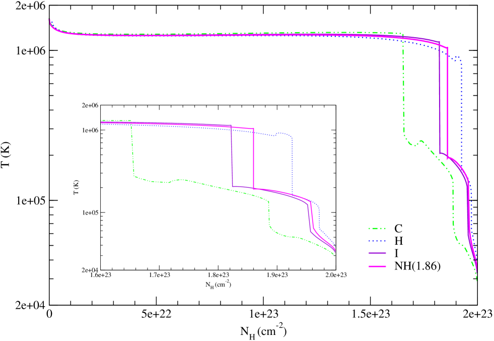
Figure 1: Temperature profile versus the column density for our reference cloud in the extreme C and H states, in the intermediate I state resulting from TITAN  in its automatic operational mode, and in the state NH(1.86) with the position of the temperature drop consistent with the conduction based criterion. Inserted box: zoom of the temperature profile on the thermal instability zone.

The extension of the instability zones and consequently the limits to the exact location of the temperature discontinuity is provided by the two extreme models, H and C, corresponding to the lowest and the highest values of the hydrogen column density measured at the discontinuity.

For our reference cloud, the values of the hydrogen column are $1.92\times 10^{23}$ cm^-2 for the state H, and $1.54\times 10^{23}$ cm^-2 for the state C (in our notations, those values correspond to the NH(1.92) and NH(1.54) states, respectively).

The temperature profiles with the sharp drops for the states C and H are shown in Fig. 1. Since the intermediate state is closer to the H state than to the C state, we will calculate the sequence of the intermediate states from NH(1.78) to NH(1.89).

For all these states we have calculated the value of the integral $A$ from Eq. 5 in the Appendix A. This requires the construction of the heating/cooling curves as function of the temperature in various layers. The curves have a complex shape, since multiple instability zones actually exist within the cloud. The integral gains a positive contribution from the beginning of the instability zone as the heating/cooling is positive, whereas, at the end of the transition region, the contribution is negative. This result is depicted in Fig. 2.

The best agreement with the condition $A=0$ is achieved for a given state NH($x$) with $1.85<x<1.87$, consistent with the real temperature drop being located somewhere between $1.85\times 10^{23}$ cm^-2and $1.87\times 10^{23}$ cm^-2. NH($x$) model computations being extremely time-consuming, we did not calculate the $1.85<x<1.87$ states very densely. Among the computed models, the NH(1.86) state offers the best agreement with the condition $A=0$.

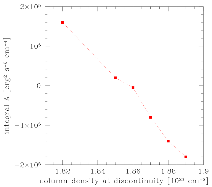
Figure 2: Variation of integral $A$ (units erg² s^-2 cm^-4) as a function of the column density (units cm^-2) for several intermediate states labeled after the adopted position of the discontinuity. The best agreement between the adopted position and the position indicated by $A=0$ is obtained for model NH(1.86).

Defining our equilibrium condition using Eq. 5 given in the Appendix, we have assumed the left-hand part of this equation to be null, i.e. $A=0$. This requires that either $F_{cond}(T_{hot})=F_{cond}(T_{cold})$, or else that both $F_{cond}(T_{hot})$ and $F_{cond}(T_{cold})$ are null (or at least negligible as compared to the integral, when it is non null). We have tested that hypothesis a posteriori: calculating the left-hand side of Eq. 4, we have found it to be negligible.

Finally, it is interesting to note that the models where the adopted temperature drop roughly coincides with the estimated location of the temperature drop from the conduction criterion are numerically stable (see Appendix B).

In addition to the adopted NH(1.86) state, we also estimated the conduction flux above and below the temperature drop for a few additional cloud states. Our results show that the energy flux carried by electrons is always at least five orders of magnitude lower than the incident radiation flux. This is also true at the cloud surface since, although the temperature is higher there, the temperature drop is quite shallow. In an effort to further test our conclusions, we have refined the spacial grid by a factor of 100, at the expense of increasing the computational time considerably; our results show that the conduction flux calculated directly from the temperature profile remain negligible. Therefore, we conclude that outside the instability zone, the electron conduction is negligible and the temperature drop is unresolved in TITAN.

3.2 Transmission spectra

In Paper I we have shown that the transmission spectra for the H and C states are considerably different, thus demonstrating the importance of a sufficiently accurate measure of the temperature drop location. Thanks to the method developed in this paper, we were able to identify the (approximate) location that is consistent with the condition resulting from the introduction of the electron conduction term. We are now capable to compare the transmission spectrum obtained for state NH(1.86) with the spectra resulting from states H and C. These were also compared with the standard I state resulting from the default TITAN mode (faster and numerically more stable than the other modes).

Figure 3 shows a pure transmitted spectra (i.e. covering factor $\sim 1$) at resolution $\nu/\Delta\nu=300$, and Table 1 the comparison of the strongest lines present in H, C, I, and NH(1.86) models. The continuum in NH(1.86) shows somewhat less absorption than in I, but the maximum difference, located around 1 keV, is never larger than 27%. The maximum relative difference between the measured lines in NH(1.86) and I models is less than 24% for the 200 strongest features. Most of the strongest lines show a difference less than 1%, because they are saturated; some lines show a 20% difference (e.g. Fe XII and Fe XIII) which is related to a change of ionization fraction, due to a different ionic column density (see Paper I). For the outward and reflected spectra (emitted in all directions but the normal), the difference between models I and NH(1.86) is again weak, i.e. less than 25%. We therefore conclude that the I model can be used safely to describe such a medium, which falls within the range of conditions valid for the Warm Absorber in AGN.

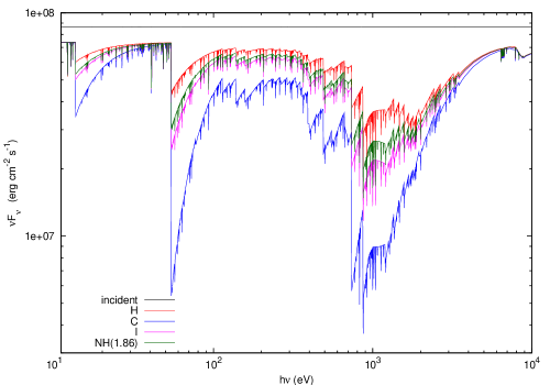
Figure 3: Transmitted continuum flux $\nu F(\nu)$ (in erg s^-1 cm^-2 s^-1) vs. Energy (in eV) for our H, C, I, and NH(1.86) models. The plotted energy range is 10 eV to 10 keV; no differences are observed in the different models outside this range. The spectral resolution $\nu/\Delta\nu$ is 300.

ION	$h\nu$	Line Flux	$|$1-I/NH(1.86)$|$
	(eV)	NH(1.86)	(%)
HI	1.020e+01	-1.2e+05	1
HI	1.209e+01	-7.2e+04	1
HeII	4.080e+01	-7.0e+04	0.2
HeII	4.836e+01	-5.7e+04	1
HI	1.275e+01	-5.4e+04	0.2
HeII	5.100e+01	-4.3e+04	1
HI	1.305e+01	-4.0e+04	0.9
FeXVII	8.260e+02	-3.9e+04	6
HeII	5.223e+01	-3.6e+04	0.5
OVIII	6.533e+02	-3.7e+04	6
CVI	3.674e+02	-3.5e+04	5
FeXV	4.366e+01	-2.7e+04	9
FeXXI	1.001e+03	-3.4e+04	20
FeXXII	1.042e+03	-3.3e+04	20
SiIX	2.066e+02	-2.5e+04	7
SiX	2.448e+02	-2.5e+04	5
FeXXII	1.110e+02	-2.6e+04	3
SXI	3.100e+02	-2.5e+04	4
SXIV	2.908e+01	-2.5e+04	0.7
SiXI	2.833e+02	-2.4e+04	5
CVI	4.354e+02	-2.6e+04	7
SiXII	2.450e+01	-2.4e+04	2
SX	2.599e+02	-2.3e+04	6
FeXX	9.336e+01	-2.5e+04	6
FeXXIII	9.334e+01	-2.4e+04	5
FeXXI	1.213e+02	-2.3e+04	3
NVII	5.001e+02	-2.4e+04	9
NeVII	2.665e+01	-2.1e+04	6
OVII	6.655e+02	-2.2e+04	0.05

Table 1: Table highlighting the differences between the transmitted spectra resulting from I and NH(1.86) models. For a small sample of 29 lines, we give the ion name, the energy of the line (eV), the line-integrated flux for NH(1.86) (arbitrary units), and the relative difference with the I model (in percent). The lines are sorted from the strongest to the weakest, as observed in model NH(1.86).

3.3 The structure of the conductive layer

Since we determined the position of the transition layer we can calculate a posteriori the structure of this sharp transition zone in a semi-analytical way, including the conduction flux. For that purpose we obtained first the heating/cooling function as a function of the temperature for the total pressure characterizing the model NH(1.86) in the transition zone. We stress that the heating/cooling is obtained for a constant presure, not constant density, as this assumption esentially influences its shape, as nicely explained in Goncalves et al. (2007). The resulting heating/cooling curve is shown in Fig. 4.

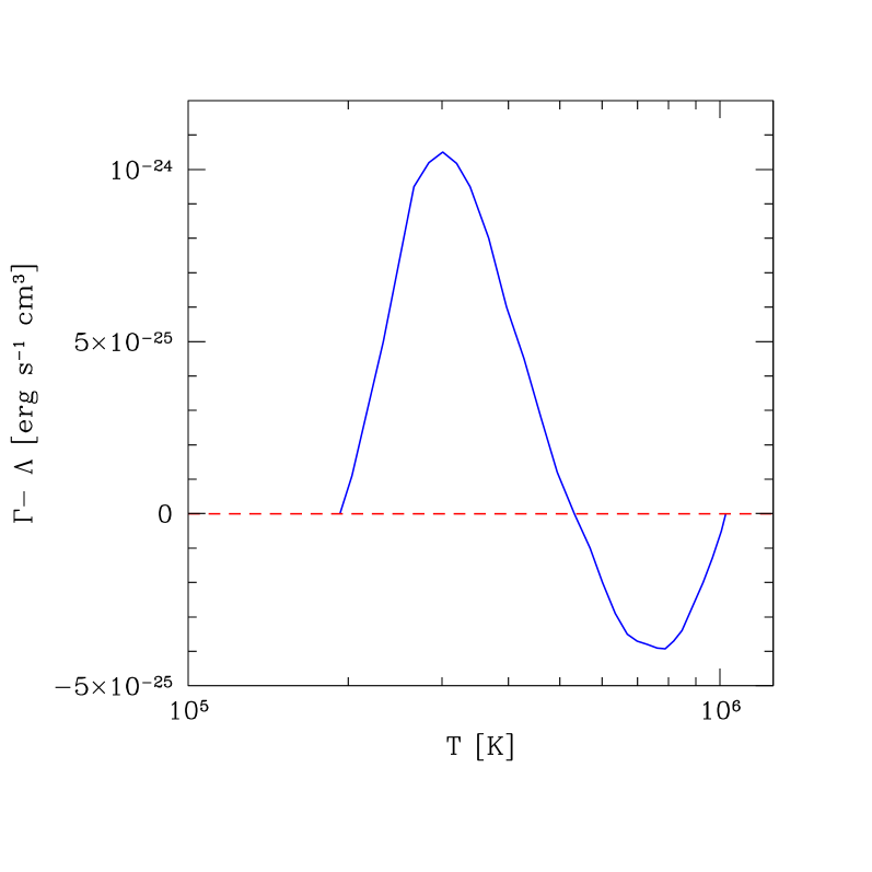
Figure 4: The heating/cooling curve for model NH(1.86) at the position of the conductive discontinuity as a function of the temperature, obtained under constant pressure condition. The curve crosses zero (radiative balance) for three values of the temperature. Compton heating as well as all atomic heating/cooling processes are included.

Having this curve, and assuming constant pressure in the sharp transition zone we can now easily obtain the conduction flux as a function of the temperature from the integral form of the conduction equation (see Eq. 4 in the Appendix and replace $T_{hot}$) and replacing $T_{hot}$ with a set of intermediate value of $T$. Next, returning to the expression for conduction flux we can obtain the spacial temperature gradient in the constant pressure zone. The resulting flux and the temperature profile are shown in Fig. 5. The hydrogen column within this zone is equal to $1.54\times 10^{20}$ cm so the zone unresolved in radiative transfer computations should not strongly contribute to the spectrum although it is not totally negligible.

In the transition zone the conductive flux is still orders of magnitude smaller than the radiative flux but nevertheless it contributes significantly to the total energy balace in this zone since the derivative of the conduction flux is large. The conductive flux balances the departure of the heating/cooling curve from zero and since the single heating or cooling mechanism gives values of order of $10^{-24}$ erg s^-1 cm³ the flux derivative is of the same order of magnitude as the heat deposit or loss, just due to the geometrical narrowness of the zone. Therefore, just comparing the two fluxes instead of their derivatives, as done e.g. by Sage & Seaton (1973) in their analysis may be misleading.

The global significance of the conduction-dominated narrow zone itself of course is affected by its narrowness, and from this point of view the simple argument of Sage & Seaton (1973) is correct and the zone does not contribute strongly to the final transmission spectra so the fact that in our numerical computations of the radiative transfer we neglected this zone completely is fully justified.

The important effect of electron conduction is, however, in the determination of the position of the discontinuity, and this is the real effect we search for, as explained in Sect. 2. Having semi-analytical results we can now check if the conduction is effective enough to move the position of the transition zone.

If the initial position of the transition zone for some reason is not consistent with the conduction criterion (see Appendix) the transition zone will move with the velocity rougly given by the ratio of the conduction flux to the local energy density, i.e. $2F_{cond}/(5n_{H}kT)\sim 10$ km s^-1. This speed is strongly subsonic. The whole size of the reference cloud where three solutions for the radiative equilibrium are possible covers the range of $3\times 10^{22}$ cm^-2 in hydrogen colun and the spatial distance of $\sim 10^{14}$ cm, i.e. the conduction flux will adjust the front position in about 3 years. Slowly moving ($v<500$ km s^-1) distant (above $\sim 3\times 10^{16}$ cm) cloud in the radiation field of an active nucleus has time to reach such equilibrium since the motion of the front due to systematically decreasing flux is slower than the effect of conduction estimated above. The fact that the irradiation in an AGN is time-dependent complicates the problem, as discussed by Chevallier et al. (2007).

A question remains whether such a narrow zone can exist and be stable. The first issue is related to the mean free path of electrons. In the likely presence of a weak magnetic field this seems to be possible. The mean free path of an electron for a micro-Gauss magnetic field is a fraction of a cm, much smaller than the size of the transition region. Stability issue is another problem. A study e.g. by Różańska (1999) in the context of disk/corona border indicated marginal stability.

However, a magnetic field may also reduce heat conduction and in this case we may strongly overestimate the conduction flux. The issue was discussed other astrophysical contexts like wind collisions but the theory is rather complex and uncertain. Recent Chandra observations of a planetary nebule PN BD+30^∘3639 by Nordon et al. (2009) suggest complex structure of such a zone, with ions penetrating the contact discontinuity boundary. The countrate in AGN observation is much lower so at present the search for such traces in AGN warm absorber is likely to be premature.

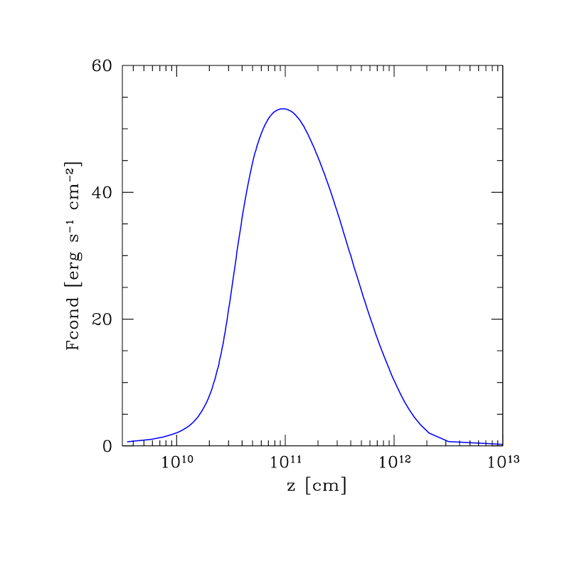
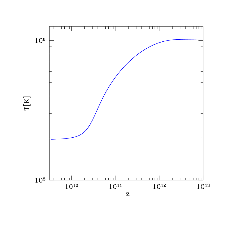
Figure 5: The spacially resolved temperature (upper panel) and conduction flux (lower panel) profiles in the transition zone obtained from semi-analytical approximation (see text). The transition is sharp in comparison with extension of a whole reference cloud $\sim 10^{15}$ cm.

4 Discussion

This study represents an important contribution to the understanding of the technical aspects behind radiative transfer computations in stratified media under total constant pressure. It is well known that an irradiated gas in constant pressure will develop thermal instabilities, if the electron conduction is neglected (e.g. Krolik et al. 1981). These instabilities appear as technical problems in radiative transfer and photoionization codes. Therefore, various codes use different approaches to address this problem.

In this paper we tested the different numerical approaches used by the TITAN code. We constructed a subset of radiative transfer solutions, all for the same column density of the cloud and the same incident radiation flux, and identified the one which is close to satisfy the equilibrium condition derived from the electron conduction theory. We found that the approximate solution obtained by the standard, automatic mode of the TITAN code provides a satisfactory representation of the transmitted spectra. We find that most line intensities resulting from this automatic mode are in agreement with the values derived from the electron conduction theory, reaching an accuracy of the order of 1%, with only a few exceptions (mostly iron lines at intermediate ionization state) where the discrepancy between the solutions reached 20%.

We have tested our methodology and hypothesis on a given cloud, described by a single set of parameters; these were chosen among the range of conditions usually met in the modeling of the X-ray ionized gas near the central regions of AGN, and are fully compatible with a Warm Absorber medium. An issue remains – that of computations based on the conduction criterion being much more time-consuming (at least by a factor 20), than the standard radiative transfer computations, which are already quite long. Therefore, it is not feasible to apply this computation method to directly obtain solutions for a grid of models, for instance. The results of this work provide, nevertheless, important evidence that the standard, automatic computing mode of the TITAN code is not strongly affected by systematical errors caused by neglecting to include the electron conduction. This is important, since constant pressure models are a much better approximation than constant density models, with applications in several physical circumstances, e.g. the Warm Absorber clouds, or the disk/corona transition zone in an accretion disk onto a black hole.

On the other hand, our analysis does not address the evolutionary aspect of the presence of thermal instability. In this paper, as in other papers devoted to the modeling of the Warm Absorber, we assumed that the very existence of the clouds (instead of a continuous wind) is a result of this instability, but we did not address the timescales for the cloud formation and its survival. A first attempt at this exercise can be found in Paper I and in Chevallier et al. (2007). Additional discussions on these aspects of the thermal instability have been reported in other contexts i.e.: the hot medium in galaxy clusters (Kim & Narayan 2003), and the multiphase interstellar medium (Inoue et al. 2006). In the case of AGN the issue of the medium fragmentation is additionally made more complex by the fact that the irradiation flux itself varies significantly in time, so the cloud can never achieve a full thermal equilibrium (e.g. Chevallier et al. 2007). Those issues are clearly beyond of the scope of the present paper.

Appendix A

We recall the main relations for energy balance with the thermal conduction effect included (see Różańska & Czerny 2000a), which are used and eventually modified for the purpose of this study. The energy balance at $z$ (i.e. which permits to compute the temperature at this position) across the boundary between the hot and cold media in the static case is given by

$$\frac{\mathrm{d}F_{cond}}{\mathrm{d}z}=n_{e}n_{H}(Q^{+}-\Lambda)\;,$$ (2)

where $Q^{+}$ and $\Lambda$ determine the heating and cooling rates of the matter by energy exchange with radiation only, respectively, and $n_{e}\sim 1.18n_{H}$ for such cosmic abundances. Note that the total density is $n=2.25n_{H}$. Note also that $Q^{+}$ and $\Lambda$ are the usual definition of volumic coefficients par particle, explaining the factor $n_{e}n_{H}$. On the left-hand side of Eq. 2 appears the conductive heat flux $F_{cond}$, defined as

$$F_{cond}=-\kappa_{0}T^{5/2}\frac{\mathrm{d}T}{\mathrm{d}z}\;,$$ (3)

where $\kappa_{0}=5.6\times 10^{-7}$ erg cm^-1 s^-1 K^-7/2 is the conductivity constant for a typical astrophysical plasma with cosmic abundances (Allen 1973). The typical value of $\Lambda$ is of order of $10^{-23}$ erg cm³ s^-1. In the code Titan, the term on left hand side of Eq. 2 is neglected while the right hand side is calculated carefully, with line and continuum emission/absorption processes.

Under the condition of constant gaseous pressure (i.e. perfect gas), we can express Eq. 2 performing an integral (Eq. 8 in Różańska & Czerny (2000a)) over the temperature in the thermal instability region from the cold solution $T_{cold}$ to the hot solution $T_{hot}$. Under the constant total (gaseous + radiative) equilibrium of our clouds $P_{tot}=P_{gas}+P_{rad}$, both gaseous and radiative pressures vary in the thermal instability region, in a non-local dependence of the temperature. This assumption cannot be done on theoretical grounds. However we observe that this variation is weak, so the non-local dependence is not drastic, and use the local value of the gaseous and radiative pressure is consistent with the way we have computed the heating and cooling curves for our code. Eq. 8 from Różańska & Czerny (2000a) becomes, when inserting the factor $n_{e}n_{H}=1.118/(2.25k)^{2}(P_{tot}-P_{rad})^{2}/T^{2}$, where $k=1.38\times 10^{-16}$ erg K^-1 is the Boltzmann constant,

$$F_{cond}^{2}(T_{cold})-F_{cond}^{2}(T_{hot})=$$ (4)

$$2\kappa_{0}\frac{1.18}{2.25^{2}k^{2}}(P_{tot}-P_{rad})^{2}\int_{T_{cold}}^{T_{hot}}(Q^{+}-\Lambda)\sqrt{T}\mathrm{d}T\,,$$

where the conductive heat flux at temperatures $T_{hot}$ and $T_{cold}$ should be small enough to be neglected. We denote by $A$ the right-hand part of Eq. 5. Usual calculation of the thermal conduction effect require $A=0$. Each quantity $F_{cond}^{2}(T_{hot})$ or $F_{cond}^{2}(T_{cold})$ should be small, as the temperature gradient outside the thermal instability zone is small. But the difference could be of the same order of magnitude than $A$. We will neglect the left-hand side of Eq. 4 and we will check the consistency of the assumption a posteriori:

$$2\kappa_{0}{{1.18}\over{2.25^{2}k^{2}}}(P_{tot}-P_{rad})^{2}\int_{T_{cold}}^{T_{hot}}(Q^{+}-\Lambda)\sqrt{T}\mathrm{d}T=A=0.$$ (5)

Appendix B

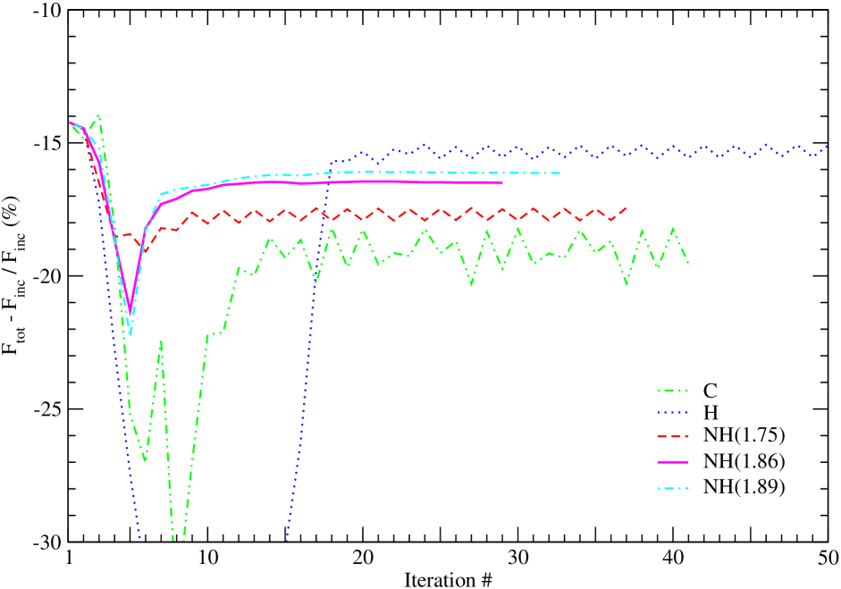
Figure 6: The convergence properties of our reference cloud as a function of the iteration number up to iteration 50, for the states H (no change up to iteration 65) C, and NH(1.86). Note that the NH(1.86) model converges more rapidly and without oscillations.

It is interesting to note that finding the exact location of the discontinuity in the model provides also a solution to some numerical problems which are met in titan used in the second (nonstandard) operational mode, used in Paper I. If we attempt to determine the type H state of the cloud (i.e. we choose always the hottest solution in the multiple solution region; see Sect. 2) we actually face the problem of the small regular oscillations in the state properties, which translate into the small but finite oscillations in the total energy balance of the cloud. To illustrate this we present in Fig 6 the dependence of our estimator of convergence, on the number of iterations for different states. The oscillations in total energy balance correspond to the oscillations in the location of the main temperature drop (see Fig. 1).

The oscillations cease to exist if we impose the position of the temperature discontinuity quite close to the position required by the conduction condition $A=0.$. Specifically, oscillations are not present in all models from NH(1.82) to NH(1.89).