Continuous frequency spectrum of the global hydromagnetic oscillations of a magnetically confined mountain on an accreting neutron star

Abstract

We compute the continuous part of the ideal-magnetohydrodynamic (ideal-MHD) frequency spectrum of a polar mountain produced by magnetic burial on an accreting neutron star. Applying the formalism developed by Hellsten & Spies (1979), extended to include gravity, we solve the singular eigenvalue problem subject to line-tying boundary conditions. This spectrum divides into an Alfvén part and a cusp part. The eigenfunctions are chirped and anharmonic with an exponential envelope, and the eigenfrequencies cover the whole spectrum above a minimum $\omega_{\mathrm{low}}$. For equilibria with accreted mass $1.2\times 10^{-6}\la M_{a}/M_{\odot}\la 1.7\times 10^{-4}$ and surface magnetic fields $10^{11}\la B_{\ast}/\mathrm{G}\la 10^{13}$, $\omega_{\mathrm{low}}$ is approximately independent of $B_{\ast}$, and increases with $M_{a}$. The results are consistent with the Alfvén spectrum excited in numerical simulations with the zeus-mp solver. The spectrum is modified substantially by the Coriolis force in neutron stars spinning faster than $\sim 100$ Hz. The implications for gravitational wave searches for low-mass X-ray binaries are considered briefly.

1 Introduction

Radio and X-ray observations suggest that the magnetic dipole moments, $\mu$, of neutron stars in accreting binaries decrease with accreted mass, $M_{a}$ (Taam & van de Heuvel, 1986; van den Heuvel & Bitzaraki, 1995). One physical mechanism capable of reducing $\mu$ by the amount observed is magnetic screening or burial (Bisnovatyi-Kogan & Komberg, 1974; Romani, 1990; Konar & Bhattacharya, 1997; Zhang, 1998; Melatos & Phinney, 2001; Choudhuri & Konar, 2002; Payne & Melatos, 2004; Lovelace et al., 2005). Magnetic burial occurs when accreting plasma, flowing inside the Alfvén radius, is channelled onto the magnetic poles of the neutron star. The hydrostatic pressure at the base of the accreted column overcomes the magnetic tension and the column spreads equatorwards, distorting the frozen-in magnetic flux (Melatos & Phinney, 2001). Self-consistent magnetohydrodynamic (MHD) equilibria respecting the flux-freezing, ideal-MHD constraint were computed by Payne & Melatos (2004), who found that the magnetic field is compressed into an equatorial belt, which confines the accreted mountain at the poles. A key result is that $\mu$ drops significantly once $M_{a}$ exceeds the critical mass $M_{c}\sim 10^{-5}M_{\odot}$. This characteristic value exceeds simple estimates based on local MHD force balance at the polar cap , i.e. without the equatorial magnetic belt (Brown & Bildsten, 1998; Litwin et al., 2001).

Counterintuitively, magnetic mountain equilibria prove to be marginally stable (Payne & Melatos, 2007; Vigelius & Melatos, 2008c). An axisymmetric mountain is susceptible to the undular submode of the Parker instability, but the instability is transitory, saturating after $\sim 10$ Alfvén times to give a nearly axisymmetric, mountain-like state, which oscillates in a superposition of small-amplitude, global, Alfvén and acoustic modes (Payne & Melatos, 2007; Vigelius & Melatos, 2008c). The magnetic line-tying boundary condition at the stellar surface is crucial in stabilizing the mountain.

The Alfvén and acoustic oscillations help to shape the gravitational wave spectrum emitted by low-mass X-ray binaries (Vigelius & Melatos, 2008a), furnishing a new observational probe of the surface magnetic structure of neutron stars. The oscillations may also manifest themselves as small, Hz-to-kHz variations in the X-ray pulse shape. Accordingly, a linear eigenmode analysis of the ideal-MHD spectrum is required to take full advantage of future gravitational-wave and X-ray timing experiments. Here, we take a first step by computing the continuous part of the ideal-MHD spectrum analytically for axisymmetric magnetic mountains, closely following the approach of Hellsten & Spies (1979).

Realistically, however, the detection of the gravitational-wave imprint from mountain oscillations will not be possible in the near future. While Advanced Laser Interferometer Gravitational Wave Observatory (Advanced LIGO) may detect the unperturbed mountain (Watts et al., 2008; Vigelius & Melatos, 2008a), the detection of modulations of the main signal from mountain oscillations will have to await next-generation interferometers. On the other hand, X-ray-profile changes can currently be measured with an accuracy of $\sim 1$ per cent (Muno et al., 2002; Hartman et al., 2008) and we know that the accretion rate changes by $\sim 10$ per cent per day. Unfortunately, the X-ray fluctuations will be only poorly frequency-matched to the mountain oscillations in general.

Generally, an inhomogenuous MHD configuration supports linear eigenmodes (Lifschitz, 1989; Goedbloed & Poedts, 2004), whose frequency spectrum divides into a discrete and a continuous part. Discrete eigenvalues are fixed by the boundary conditions. Continuous eigenvalues arise from singularity in the underlying Sturm-Liouville problem, which allows the boundary conditions to be satisfied for any eigenvalue within a range.

In earlier work, stochastically excited mountain oscillations were investigated numerically by perturbing equilibrium stars with different $M_{a}$ in the ideal-MHD solver zeus-mp (Hayes et al., 2006), and computing the spectrum (Payne & Melatos, 2007; Vigelius & Melatos, 2008c). However, this approach is restricted to the subset of the full MHD spectrum resolved by zeus-mp and is computationally expensive. In this article, we attack the problem analytically. The article is organised as follows. In section 2, we introduce curvilinear field line coordinates to describe the equilibrium and establish the associated metric. We derive the linearized, ideal-MHD equations in these coordinates in section 3, extending the analysis by Hellsten & Spies (1979) to include the gravitational field of a central point mass. The continuous frequency spectrum and the corresponding eigenfunctions are evaluated in section 4, as a function of $M_{a}$ and the magnetic field strength before burial. We conclude by discussing the implications for gravitational wave observations of accreting millisecond pulsars in section 5.

2 Hydromagnetic equilibrium

The equilibrium structure of a magnetically confined mountain in ideal MHD is described by the force balance equation

$$\nabla P-(\nabla\times\mn@boldsymbol{B})\times\mn@boldsymbol{B}=N\mn@boldsymbol{g},$$ (1)

supplemented by $\nabla\mn@boldsymbol{\cdot}\mn@boldsymbol{B}=0$ and an equation of state $P(N)$, which we take to be isothermal: $P=c_{s}^{2}N$. Here, P, $\mn@boldsymbol{B}$, $N$, $\mn@boldsymbol{g}$, and $c_{s}$ denote the pressure, magnetic field, mass density, gravitational acceleration, and isothermal sound speed, respectively.

If we introduce a cylindrical coordinate system $(r,\varphi,z)$ and assume axisymmetry, we can write

$$\mn@boldsymbol{B}=\nabla\varphi\times\nabla\Psi,$$ (2)

where $\Psi$ is the magnetic flux, measured in G cm². Payne & Melatos (2004) computed unique, self-consistent, MHD equilibria by solving (1) in spherical coordinates subject to the flux-freezing constraint of ideal MHD. In this article, we convert these solutions to cylindrical coordinates before constructing the associated field line coordinates.

Throughout this article, we work in cgs-like units, such that $\mu_{0}=1$. Furthermore, we normalize the isothermal sound speed and the gravitational constant, viz. $c_{s}=G=1$.

2.1 Field line coordinates

A magnetic mountain is created by continuously deforming a dipole magnetic field during the accretion process. The flux surfaces are closed at all times, a topology that is preserved even for a uniform $B_{\varphi}\neq 0$. We can therefore introduce orthogonal curvilinear coordinates $(\Psi,\eta,\varphi)$, called field line coordinates, which “follow” the shape of the flux surface. In these coordinates, $\eta$ measures arc length along a magnetic field line, normalized to the domain $0\leq\eta\leq 1$, where $\eta=0$ corresponds to the footpoint at the surface, and $\eta=1$ corresponds to the outer radial boundary or, when the field line is closed, to the surface. $\Psi$ is the flux function in (2) and $\varphi$ is the usual azimuthal angle in cylindrical coordinates. In the field line coordinates, the metric becomes (Hellsten & Spies, 1979)

$$\mathrm{d}s^{2}=\frac{1}{r^{2}B^{2}}\mathrm{d}\Psi^{2}+J^{2}B^{2}\mathrm{d}\eta^{2}+r^{2}\mathrm{d}\varphi^{2},$$ (3)

with the Jacobian $J$ given by

$$J=(\mn@boldsymbol{B}\mn@boldsymbol{\cdot}\nabla\eta)^{-1}.$$ (4)

Note that, for $B_{\varphi}=0$, we have $J=B^{-1}$. However, in keeping with Hellsten & Spies (1979) we uphold the more general notation in order to facilitate the inclusion of a toroidal field component in future work.

The contravariant components of the force balance equation (1) in the $\Psi$ and $\eta$ directions read respectively

$$\frac{\partial P}{\partial\Psi}+\frac{1}{J}\frac{\partial}{\partial\Psi}(JB^{2})=A_{0}N,$$ (5)

and

$$\frac{\partial P}{\partial\eta}=A_{1}N.$$ (6)

The gravitational acceleration is directed radially inward to the centre of the star (mass $M$). Ignoring self gravity, we have

$$\mn@boldsymbol{g}=A_{0}\mn@boldsymbol{e}_{\Psi}+A_{1}\mn@boldsymbol{e}_{\eta},$$ (7)

with

$$A_{0}=\mn@boldsymbol{g}\mn@boldsymbol{\cdot}\mn@boldsymbol{e}_{\Psi}=-\frac{M}{(r^{2}+z^{2})^{3/2}}\left(r\frac{\partial r}{\partial\Psi}+z\frac{\partial z}{\partial\Psi}\right),$$ (8)

and

$$A_{1}=\mn@boldsymbol{g}\mn@boldsymbol{\cdot}\mn@boldsymbol{e}_{\eta}=-\frac{M}{(r^{2}+z^{2})^{3/2}}\left(r\frac{\partial r}{\partial\eta}+z\frac{\partial z}{\partial\eta}\right).$$ (9)

Payne & Melatos (2004) took $\mn@boldsymbol{g}$ to be constant to simplify the analysis, but we prefer to use Eqs. (8) and (9) to allow direct comparison with the numerical results of Payne & Melatos (2007) and Vigelius & Melatos (2008c).

For later comparison, we note that (5) and (6) become formally identical to Eqs. (13) and (14) of Hellsten & Spies (1979) for a stationary fluid in the absence of gravity, rotating around the $z$ axis with constant angular velocity $\Omega$, if we substitute

$$A_{0}=\Omega^{2}r\frac{\partial r}{\partial\Psi},$$ (10)

and

$$A_{1}=\Omega^{2}r\frac{\partial r}{\partial\eta}.$$ (11)

Of course, we cannot write the centrifugal force in the form (7), as it is not radial, so the substitution (10) and (11) is algebraic, not physical.

2.2 Accreted magnetic mountain

Figure 1: Hydromagnetic structure of a magnetically confined mountain with $M_{a}=M_{c}$ in spherical polar and field line coordinates. The left panel displays the density contours (dashed) $\log_{10}(N/N_{0})=-13,-12,-11,-10.7,-10.5,-10.3$, with $N_{0}=5.2\times 10^{19}$ g cm^-3, the magnetic field strength contours (dotted) $\log_{10}(B/B_{0})=-7,-6,-5.5$, with $B_{0}=2.55\times 10^{18}$ G, and the magnetic field lines (solid) with footpoints at $R=R_{\ast}$ and $\theta=0.10,0.12,0.15,0.20,0.39,0.79$, in the $R$-$\theta$ plane, where $(R,\theta,\varphi)$ are standard spherical polar coordinates. The right panel presents the same information in the $\Psi$-$\eta$ plane, where $\Psi$ is normalized to the flux surface that closes at the inner edge of the accretion disk $\Psi_{a}$, and $\eta$ is the arc length along a field line, normalized to $0\leq\eta\leq 1$.

Throughout this paper, we study magnetic mountain equilibria on the surface of a curvature-downscaled star with radius $R_{\ast}^{\prime}=2.7\times 10^{3}$ cm and mass $M_{\ast}^{\prime}=1.0\times 10^{-5}M_{\odot}$. The downscaling transformation preserves the equilibrium shape of the mountain [exactly in the small $M_{a}$ limit and approximately in the large $M_{a}$ limit; see Payne & Melatos (2004); Vigelius & Melatos (2008c)], as long as the hydrostatic scale height $h_{0}=53.82$ cm keeps its original value for a realistic star. Base units are $M_{0}=8.1\times 10^{24}$ g, $N_{0}=5.2\times 10^{19}$ g cm^-3, $B_{0}=7.2\times 10^{17}$ G, and $\tau_{0}=5.4\times 10^{-7}$ s, for mass, density, magnetic field, and time respectively. In order to upscale the frequencies back to a realistic neutron star, we employ the relation $\omega^{2}\propto(h_{0}/R_{\ast})^{2}$ (Payne & Melatos, 2006). While, strictly speaking, this relation only applies to waves travelling latitudinally, we note that the field lines are predominantly parallel to the neutron star surface (Fig. 1, left panel) and the error will be small.

An equilibrium configuration with $M_{a}=M_{c}=1.2\times 10^{-4}M_{\odot}$ is displayed in Fig. 1. $M_{c}$ denotes the critical accreted mass beyond which the magnetic dipole moment is substantially reduced (Payne & Melatos, 2004). The left panel shows the density contours (dashed) and the magnetic field lines (solid), i.e. the flux surfaces $\Psi=\mathrm{const}$, projected into a meridonial plane. The equilibrium configuration extends over $0\leq\tilde{x}=(R-R_{\ast})/h_{0}\leq 10$ and $0\leq\theta\leq\pi$, where $R$ measures the radius in spherical polar coordinates, and $\theta$ is the colatitude. North-south symmetry is assumed. The mountain is confined to the magnetic pole and the distorted magnetic belt is clearly visible at $\theta\geq 0.5$ and $r\geq 52$. The right panel shows the same plot in the $\Psi$-$\eta$ plane. Of course, the field lines are projected onto straight lines in this plot. The density contours appear distorted since $\eta$ is normalized to the domain $0\leq\eta\leq 1$.

Contours of $B$ are plotted as dotted curves in both panels of Fig. 1 for $\log_{10}(B/B_{0})=-7,-6,-5.5$. The magnetic belt with its enhanced magnetic field is clearly visible between $0.6\leq\theta\leq 1.4$ in the left panel. The dotted curves trace out isosurfaces of magnetic pressure and are therefore useful for visualizing the Lorentz force confining the mountain.

3 Global linear MHD oscillations

We now consider the behaviour of small-amplitude perturbations of the magnetic mountain equilibria described in section 2. The linearized equations of ideal MHD are projected onto the field line coordinate system in section 3.1. The singularities in these equations, which determine the form of the continuous MHD spectrum, are located in section 3.2.

3.1 Equations of motion

Following the notation and approach of Hellsten & Spies (1979), we expand the velocity and magnetic field perturbations in terms of their contravariant vector components:

$$\mn@boldsymbol{v}=v^{\Psi}\mn@boldsymbol{e}_{\Psi}+v^{\eta}\mn@boldsymbol{e}_{\eta}+v^{\varphi}\mn@boldsymbol{e}_{\varphi},$$ (12)

$$\mn@boldsymbol{b}=b^{\Psi}\mn@boldsymbol{e}_{\Psi}+b^{\eta}\mn@boldsymbol{e}_{\eta}+b^{\varphi}\mn@boldsymbol{e}_{\varphi}.$$ (13)

As in any curvilinear coordinate system, the components do not have the same units in general, e.g. $v^{\Psi}$ and $v^{\varphi}$ have units G cm² s^-1 and s^-1 respectively, since $\mn@boldsymbol{e}_{\Psi}$ and $\mn@boldsymbol{e}_{\varphi}$ have units (cm G)^-1 and cm respectively. The total pressure perturbation is defined as

$$\pi=p+\mn@boldsymbol{B}\mn@boldsymbol{\cdot}\mn@boldsymbol{b}={n}+JB^{2}b^{\eta},$$ (14)

where $p$ denotes the hydrostatic pressure perturbation.

We then Fourier decompose the perturbed variables with respect to time and $\varphi$, e.g. $\mn@boldsymbol{v}\propto\exp[\mathrm{i}(-\omega t+m\varphi)]$, recalling that the equilibrium is assumed to be axisymmetric. Thus we can write down the components of the linearized momentum balance equation,

$$0 = \frac{\omega^{2}Nv^{\Psi}}{r^{2}B^{2}}-\frac{\mathrm{i}\omega A_{0}{n}x}{r^{2}B^{2}}$$ (15)

$$+\mathrm{i}\omega\frac{\partial\pi}{\partial\Psi}+\frac{\mathrm{i}\omega}{J}b^{\eta}\frac{\partial}{\partial\Psi}(J^{2}B^{2})-\frac{\mathrm{i}\omega}{J}\frac{\partial}{\partial\eta}\left(\frac{b^{\Psi}}{r^{2}B^{2}}\right),$$

$$0 = \omega^{2}NJ^{2}B^{2}v^{\eta}-\mathrm{i}\omega A_{1}{n}$$ (16)

$$+\mathrm{i}\omega\frac{\partial\pi}{\partial\eta}-\mathrm{i}\omega\frac{\partial}{\partial\eta}\left(JB^{2}b^{\eta}\right)-\mathrm{i}\omega b^{\Psi}\frac{\partial}{\partial\Psi}(JB^{2}),$$

$$0 = \omega^{2}Nr^{2}v^{\varphi}-\omega m\pi-\frac{\mathrm{i}\omega}{J}\frac{\partial}{\partial\eta}\left(r^{2}b^{\varphi}\right),$$ (17)

the components of the linearized induction equation, $\partial\mn@boldsymbol{b}/\partial t=\nabla\times(\mn@boldsymbol{v}\times\mn@boldsymbol{B})$,

$$\mathrm{i}\omega b^{\Psi}+\frac{1}{J}\frac{\partial v^{\Psi}}{\partial\eta}=0,$$ (18)

$$\mathrm{i}\omega b^{\eta}-\frac{1}{J}\left(\frac{\partial v^{\Psi}}{\partial\Psi}+\mathrm{i}mv^{\varphi}\right)=0,$$ (19)

$$\mathrm{i}\omega b^{\varphi}+\frac{1}{J}\frac{\partial v^{\varphi}}{\partial\eta}=0,$$ (20)

and the linearized mass continuity equation, $\partial n/\partial t+\nabla\mn@boldsymbol{\cdot}(N\mn@boldsymbol{v})=0$,

$$\mathrm{i}\omega n = \mathrm{i}\omega JNb^{\eta}+N\frac{\partial v^{\eta}}{\partial\eta}$$ (21)

$$+\left(\frac{\partial N}{\partial\Psi}+\frac{N}{J}\frac{\partial J}{\partial\Psi}\right)v^{\Psi}+\left(\frac{\partial N}{\partial\eta}+\frac{N}{J}\frac{\partial J}{\partial\eta}\right)v^{\eta}.$$

Equations (15)–(21) are derived by writing down the vector operators in the curvilinear coordinate system, e.g.

$$\nabla f=(rB)^{2}\frac{\partial f}{\partial\Psi}\mn@boldsymbol{e}_{\Psi}+\frac{\partial f}{\partial\eta}\mn@boldsymbol{e}_{\eta}+\frac{1}{r^{2}}\frac{\partial f}{\partial\varphi}\mn@boldsymbol{e}_{\varphi}.$$ (22)

3.2 Singular eigenvalue problem

Equations (15)–(21) can be cast into the form (Hellsten & Spies, 1979)

$$\textbf{{C}}\frac{\partial\mn@boldsymbol{X}}{\partial\Psi}+\textbf{{D}}\mn@boldsymbol{X}+\textbf{{E}}\mn@boldsymbol{Y}=0,$$ (23)

$$\textbf{{F}}\mn@boldsymbol{Y}+\textbf{{G}}\mn@boldsymbol{X}=0.$$ (24)

In (23) and (24), $\mn@boldsymbol{X}$ is a 2-vector with elements $v^{\Psi}$ and $\pi$, while $\mn@boldsymbol{Y}$ is the five-vector $(v^{\eta},v^{\varphi},b^{\Psi},b^{\eta},b^{\varphi})^{\mathrm{T}}$. C and D are matrices, while E, F, and G are differential matrix operators involving ordinary derivatives in $\eta$. Using (24), $\mn@boldsymbol{Y}$ can be eliminated from (23) to give

$$\frac{\partial\mn@boldsymbol{X}}{\partial\Psi}+\textbf{{C}}^{-1}(\textbf{{D}}-\textbf{{E}}\textbf{{F}}^{-1}\textbf{{G}})\mn@boldsymbol{X}=0.$$ (25)

The continuous part of the frequency spectrum consists of the values of $\omega$ for which (25) becomes singular at a flux surface. This happens when either

$$\textbf{{C}}\mn@boldsymbol{X}=0$$ (26)

or

$$\textbf{{F}}\mn@boldsymbol{Y}=0$$ (27)

have nontrivial solutions at some $\Psi=\Psi_{0}$. The flow continuum, equation (26), has only the trivial eigenvalue $\omega=0$. Equation (27) defines the Alfvén and cusp continua. It can be rewritten in the form (Hellsten & Spies, 1979)

$$\omega^{2}\textbf{{P}}\mn@boldsymbol{\eta}+\textbf{{L}}\mn@boldsymbol{\eta}=0,$$ (28)

where $\mn@boldsymbol{\eta}=(Jv^{\eta}$, $v^{\varphi})^{\mathrm{T}}$ and the matrices P and L are given by

$$\textbf{{P}}=N\left(\begin{array}[]{cc}B^{2}&0\\ 0&r^{2}\\ \end{array}\right),$$ (29)

$$\textbf{{L}}=\left[\begin{array}[]{ccc}\mn@boldsymbol{B}\mn@boldsymbol{\cdot}\nabla\left(\frac{PB^{2}}{B^{2}+P}\mn@boldsymbol{B}\mn@boldsymbol{\cdot}\nabla\right)+A&0\\ 0&\mn@boldsymbol{B}\mn@boldsymbol{\cdot}\nabla\left(r^{2}\mn@boldsymbol{B}\mn@boldsymbol{\cdot}\nabla\right)\end{array}\right],$$ (30)

with

$$A=\mn@boldsymbol{B}\mn@boldsymbol{\cdot}\nabla\left(\frac{B^{3}NA_{1}}{B^{2}+P}\right)-BA_{1}\mn@boldsymbol{B}\mn@boldsymbol{\cdot}\nabla N+\frac{B^{2}N^{2}A_{1}^{2}}{B^{2}+P}.$$ (31)

The eigenvalue equation (28) decouples into two second-order, ordinary differential equations (involving derivatives $\mn@boldsymbol{B}\mn@boldsymbol{\cdot}\nabla=B\mathrm{d}/\mathrm{d}\eta$), one for the Alfvén continuum and one for the cusp continuum. The problem is self-adjoint (Hellsten & Spies, 1979), so the eigenvalues $\omega^{2}$ are real. In the absence of gravity ($A=0$), the operator L is negative and both continua are real ($\omega^{2}\geq 0$). Gravity provides a constant offset $A$, such that the Alfvén continuum is stable while the cusp continuum may be unstable. We note that the cusp continuum is the two-dimensional equivalent of the slow magnetosonic continuum in a one-dimensional, gravitating plasma slab (see section 4.2 and references therein for a full discussion).

4 Continuous spectrum of a magnetic mountain

4.1 Algorithm

We solve equation (28) numerically for the continuous spectrum by following the procedure below.

1. We compute the axisymmetric Grad-Shafranov equilibrium, employing an iterative relaxation algorithm developed by Payne & Melatos (2004) (see section 2.2).

2. The magnetic field equation, $\mathrm{d}\mn@boldsymbol{r}/\mathrm{d}\eta=\mn@boldsymbol{B}(\mn@boldsymbol{r})$, is integrated via a fourth order Runge-Kutta algorithm (Press et al., 1986) to obtain field lines $r=r(\eta,\Psi_{0})$, $z=z(\eta,\Psi_{0})$ starting from different footpoints $\Psi_{0}$ at the stellar surface.

3. The field values and their derivatives are evaluated along the field lines. The entries in P and L are computed by spline interpolation in $\eta$.

4. We find $\omega^{2}$ and the associated eigenfunction by using a shooting algorithm (Press et al., 1986) to integrate (28) separately for the Alfvén and cusp continua. The integrator is fourth-order Runge-Kutta with adaptive step size control.

The boundary conditions for the eigenfunctions along any field line ($\Psi_{0},\varphi_{0}$), are:

$$\mathrm{(i)}\;Jv^{\eta}(\eta=0)=v^{\varphi}(\eta=0)=0,\;v^{\eta}(\eta=1)=v^{\varphi}(\eta=1)=0$$

when the field line is closed, or

$$\mathrm{(ii)}\;\partial_{\eta}(Jv^{\eta})(\eta=1)=\partial_{\eta}v^{\varphi}(\eta=1)=0$$

when the field line leaves the integration area, consistent with Payne & Melatos (2007) and Vigelius & Melatos (2008c). The boundary conditions at the stellar surface enforce line tying, while the zero-gradient outer boundary condition crudely approximates the magnetosphere-accretion disk coupling [cf. the discussion in Vigelius & Melatos (2008c)].

We present the eigenfunctions $Jv^{\eta}$ and $v^{\varphi}$ for four selected fieldlines in section 4.2, two leaving the integration volume and two returning to the surface. The continuous spectrum and its dependence on the accreted mass $M_{a}$ and surface magnetic field strength $B_{\ast}$ are discussed in section 4.3.

4.2 Eigenfunctions

We preface this subsection by briefly reviewing the physical origin of the continuous spectrum in a plane-parallel, gravitating (but not self-gravitating) plasma slab. This analogous system can be treated analytically and is helpful when interpreting the results for a magnetic mountain. Here, we follow the exposition in Goedbloed & Poedts (2004).

Consider an infinite slab in Cartesian coordinates $(x,y,z)$, whose magnetic flux surfaces are perpendicular to the gravitational acceleration (directed along the $x$-axis). We render the problem one-dimensional by assuming that all equilibrium quantities $N(x)$ and $\mn@boldsymbol{B}(x)=B(x)\mn@boldsymbol{e}_{y}$ depend only on the height $x$ or, equivalently, on $\Psi(x)$. In this case, equation (25) exhibits a genuine singularity, i.e. the associated eigenfunctions become singular, when the eigenvalue $\omega^{2}$ equals the local Alfvén or slow magnetosonic frequency, i.e. either $\omega^{2}=\omega^{2}_{\mathrm{A}}(x)=(\mn@boldsymbol{k}_{0}\mn@boldsymbol{\cdot}\mn@boldsymbol{B})^{2}/N$ or $\omega^{2}=\omega^{2}_{\mathrm{S}}(x)=N\omega^{2}_{\mathrm{A}}(x)/(N+B^{2})$. The horizontal wave vector $\mn@boldsymbol{k}_{0}$ is the projection of $\mn@boldsymbol{k}$ onto the magnetic flux surface. All eigenfunctions can be written as $\xi(\mn@boldsymbol{x})=\xi_{0}(\Psi)\exp[\mathrm{i}(k_{y}y+k_{z}z)]$, with $k_{0}=(k_{y}^{2}+k_{z}^{2})^{1/2}$. It can be shown that $v^{\Psi}$ is then square integrable, involving a logarithmic singularity, while $v^{z}$ is not square integrable for the Alfvén continuum, and $v^{y}$ is not square integrable for the slow modes. In addition, (25) exhibits an apparent singularity, when $\omega^{2}$ equals the local magnetosonic turning point frequencies, i.e. the slow and fast magnetosonic frequencies for $k_{x}=0$. In this case, the eigenfunctions remain finite.

The mountain equilibrium exhibits logarithmic singularities in $\mn@boldsymbol{X}$ and $\mn@boldsymbol{Y}$ for the Alfvén and cusp continuum Hellsten & Spies (1979). Naturally, in a realistic scenario perturbations are damped by nonideal effects such as viscosity and resistivity and singular eigenfunctions cannot arise. For example, resistivity will limit the maximum fractional amplitude of a magnetic perturbation to $\delta B/B\leq\ln[(\tau_{\mathrm{C}}\eta)^{1/2}]$, where $\tau_{\mathrm{C}}$ is a characteristic time scale and $\eta$ is the resistivity. If we choose $\tau_{\mathrm{C}}=\tau_{\mathrm{A}}=2.2\times 10^{-2}$ cm s^-1 and $\eta=1.3\times 10^{27}$ (Vigelius & Melatos, 2008b) we find $\delta B/B\la 30$. Of course, the linear approximation breaks down at such a high fractional amplitude.

Figure 2: Toroidal velocity eigenfunctions $v^{\varphi}$ of the Alfvén continuum for a magnetic mountain with accreted mass $M_{a}=M_{c}=1.2\times 10^{-4}M_{\odot}$. The foot points of the field lines ➀, ➁, ➂, and ➃ are at $\theta=0.1,0.2,0.6,1$ rad (left panel, tracing the field lines of the mountain in the meridional plane). The right panels graph $v^{\varphi}$ against arc length, $\eta$, along the four field lines (top to bottom) for node numbers $n=0$ (left), 1 (middle), 30 (right). $h_{0}=53.82$ cm is the characteristic scale height (units of axes in left panel) and $c_{s}=10^{8}$ cm s^-1 is the sound speed. $\eta$ is normalized to the length of the field line, such that $0\leq\eta\leq 1$.

We are now ready to apply these ideas to the continuous spectrum of a two-dimensional, magnetically confined mountain. In a two-dimensional system, all eigenfunctions are functions of $\Psi$ and $\eta$. Fig. 2 (right panels) shows the eigenfunctions $v^{\varphi}(\eta)$ for the Alfvén continuum [lower row of Eq. (28)] of an accreted mountain with $M_{a}=M_{c}$. The foot points of the field lines are at $\theta=0.1,0.2,0.6,1$ rad, corresponding to $\Psi_{0}/\Psi_{a}=0.03,0.12,0.96,2.12$. Here, $\Psi_{a}$ is the flux surface that closes at the inner edge of the accretion disk. The field lines are traced out and labelled in the left panel. The right panels show $v^{\varphi}(\eta)$ for the same field lines (top to bottom) for different numbers $n=0,1,30$, where $n$ equals the number of nodes in the eigenfunction.

Field lines ➀ and ➁ leave the integration volume, while field lines ➂ and ➃ close back onto the surface. Field line ➀ exhibits only small curvature. Consequently, $v^{\varphi}$ is sinusoidal. Its envelope increases exponentially $\propto\exp(1.5\eta)$ (best seen in the rightmost panel). Its wavelength also increases with $\eta$, which can be understood by noting that the Alfvén speed $v_{\mathrm{A}}\propto\exp(4.5\eta)$ increases towards the outer boundary. In contrast, field line ➁ runs parallel to the stellar surface until it takes a sharp turn at $\eta\approx 0.8$. Thus, $v^{\varphi}$ is a sine wave whose amplitude and wavelength remain constant until the curvature term $\mn@boldsymbol{B}\cdot\nabla$ changes at the bend, sharply increasing the amplitude and the wavelength.

The closed field lines ➂ and ➃ behave like field line ➁. Line ➂ shows a spiky feature at $\eta=0.5$ (equator) due to the change of curvature locally. Line ➃ is almost a perfect sine wave for all $\eta$. Recall that, in a plane-parallel slab, $N$ and $B$ (and consequently $v_{\mathrm{A}}$) remain constant for all $\eta$. The eigenfunctions are hence pure sine waves with the dispersion relation $v_{\mathrm{A}}=\omega/k$. We discuss this dispersion relation quantitatively in the next section.

Figure 3: Field-aligned velocity eigenfunctions $Jv^{\eta}$ of the cusp continuum for a magnetic mountain with accreted mass $M_{a}=M_{c}=1.2\times 10^{-4}M_{\odot}$. The foot points of the field lines ➀, ➁, ➂, and ➃ are at $\theta=0.1,0.2,0.6,1$ rad (left panel, tracing the field lines of the mountain in the meridional plane). The right panels graph $Jv^{\eta}$ against arc length, $\eta$, along the four field lines (top to bottom) for node numbers $n=0$ (left), 1 (middle), 30 (right). $h_{0}=53.82$ cm is the characteristic scale height (units of axes in left panel) and $c_{s}=10^{8}$ cm s^-1 is the sound speed. $\eta$ is normalized to the length of the field line, such that $0\leq\eta\leq 1$.

The eigenfunctions $Jv^{\eta}$ of the cusp continuum, displayed in Fig. 3 (right panels), behave similarly. Field lines ➀ and ➁ run parallel to the stellar surface until they bend radially outwards. Along these field lines, $Jv^{\eta}$ is essentially sinusoidal, with a sharp rise in amplitude at $\eta\approx 0.4$ and $\eta\approx 0.8$ respectively. This behaviour can be explained by the presence of the coefficient $NB^{2}/(B^{2}+N)$, which contains the partial hydrodynamic pressure (the factor $B^{2}$ comes in since we compute $Jv^{\eta}$ instead of $v^{\eta}$), which is absent in the equations for the Alfvén continuum. A comparison with Fig. 1 shows that $B$ and $N$ flatten out considerably at $\eta=0.4$ ($\eta=0.8$) for field line ➀ (➁). Consequently, the derivative of the coefficient is steep up to that point and becomes negligible thereafter. Field lines ➂ and ➃ behave essentially like their Alfvén counterparts, showing the same sharp spike at $\eta=0.5$ as lines ➀ and ➁. Remember that the field lines ➂ and ➃  cover only one hemisphere, i.e. $\eta=1$ corresponds to the equator (see Fig. 1).

We summarize our results so far. The eigenfunctions for the Alfvén continuum are sine waves with an exponential envelope. The wave length increases with $\eta$ due to the increase in the Alfvén speed. The eigenfunctions of the cusp continuum show a characteristic spike at the point where the field lines point radially outwards (and, less distinctly, at the equator for the closed field lines). This spike is a consequence of the flattening out of the $\eta$ profile of the partial hydrodynamic pressure.

4.3 Eigenvalues

We now evaluate the frequency spectrum for the magnetic mountain in Figs. 2 and 3 by computing $\omega^{2}$ for polar (footpoint at $\theta=0.01$ rad) and equatorial (footpoint at $\theta=1.6$ rad) field lines. Since $B(R=R_{\ast})$ decreases monotonically with $\Psi$, these two field lines bracket the continuous spectrum of the whole configuration. The results in section 4.2 for the four field lines in Figs. 2 and 3 do not show any evidence for a spectrum that folds over onto itself, a feature in some other MHD systems [cf. the discussion in Goedbloed & Poedts (2004)]. The spectrum folds onto itself when the characteristic speeds (Alfvén and slow-magnetosonic in the plane parallel slab) have local extrema in the $\Psi$ range considered.

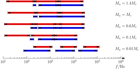
Figure 4: Alfvén (red bands) and cusp (blue bands) continuous frequency spectrum (in Hz) for magnetic mountains with (from top to bottom) $M_{a}/M_{c}=1.4,1,0.6,0.1,0.01$, computed for the node numbers (left bands to right bands) $n=0,10,100$.

Fig. 4 displays $\omega^{2}$ for $M_{a}/M_{c}=1.4,1,0.6,0.1,0.01$. We upscale all frequencies to a realistic neutron star according to $\omega^{2}\propto(h_{0}/R_{\ast})^{2}$ (Vigelius & Melatos, 2008c). The Alfvén (cusp) continuum is drawn in red (blue), as a shaded interval with double-headed arrows, for node numbers $n=0,10,100$. We stress that the gaps appearing in Fig. 4 stem from our choices of $n$; in fact, the whole spectrum $\omega^{2}\geq\omega^{2}_{\mathrm{min}}$ is covered without gaps by nodes $n\geq 0$. Furthermore, both the Alfvén and the cusp continua for different $n$ overlap. Overlap is common in some MHD systems, where multiple degeneracies of the eigenfunctions occur.

Let us compare the results in Fig. 4 to the frequency spectrum of a plane parallel slab. We remind the reader that, in a one-dimensional system like the plane-parallel slab, the spectra for different $n$ are defined by the dispersion relations given in paragraph two of section 4.2, since the equilibrium values and thus the coefficients of equation (28) do not depend on $\eta$. The lower bound for the Alfvén continuum is measured from Fig. 4 to be $\omega_{\mathrm{A,low}}/(2\pi\,\mathrm{Hz})=15.6$ for $M_{a}/M_{c}=1$. At the same time, the local Alfvén frequency for the polar field line, lies in the range $3.39\leq\omega_{\mathrm{A}}/(2\pi\,\mathrm{Hz})\,\leq 55.38$. Our aim is to pick the $n=0$ mode, so we assume $k_{0}\approx 1/h_{0}$. In our two-dimensional system, $\omega^{2}_{\mathrm{S}}$ and $\omega^{2}_{\mathrm{A}}$ are both functions of $\eta$. The first grid cell is centered at $\theta=0.01$ rad and hence determines the lowest polar field line that we can choose. This field line runs almost parallel to the $z$ axis, i.e. $r\approx\mathrm{const}$. Hence, the bottom row of (28) reduces to the dispersion relation for Alfvén waves. Consequently, $\omega_{\mathrm{A,low}}$ lies in the range of the local Alfvén frequencies. On the other hand, we can write down the dispersion relation for the cusp continuum assuming that $N$ and $B$ do not depend on $\eta$, viz. $\omega^{2}=\omega_{\mathrm{S}}^{2}-A/(NB^{2})$. The singular frequencies are offset by a constant due to the gravitational force. We compute $\omega(\eta)$ for the polar field line to be $154\leq\omega/(2\pi\,\mathrm{Hz})\leq 366$. Again, we find that $\omega_{\mathrm{C,low}}/(2\pi\,\mathrm{Hz})=189$ (cusp continuum) lies in this range.

For completeness, we display $\omega$ for the four field lines in section 4.2 as a function of the node number $n$ in Fig. 5. The Alfvén (cusp) eigenfrequencies are plotted as plus (star) symbols. For field lines ➀ and ➁, we find $\omega_{\mathrm{C}}>\omega_{\mathrm{A}}$, consistent with the discussion in the previous paragraph. However, field lines ➂ and ➃ obey $\omega_{\mathrm{A}}>\omega_{\mathrm{C}}$. The reason is that the latter fieldlines stay close to the surface. As a consequence, the constant offset, which is set by the gravitational force, is on average $\approx 2.5$ times lower for ➂ and ➃, compared to ➀ and ➁. We find $\omega_{\mathrm{A}}\rightarrow\omega_{\mathrm{C}}$ for $n\rightarrow 0$ for ➂ and ➃ , because $A$ is neglible in this case and the eigenfrequencies depend on the node number as $\omega^{2}\propto n^{2}$ with different coefficients for $\omega_{\mathrm{A}}$ and $\omega_{\mathrm{C}}$.

Figure 5: Alfvén (star) and cusp (plus) eigenfrequencies for a magnetic mountain with $M_{a}=M_{c}$ and $B_{\ast}=10^{12}$ G for the four field lines ➀–➃ in section 4.2 (four panels, labelled at top left) as a function of node number $0\leq n\leq 10$.

We are now in a position to explore the dependence of $\omega_{\mathrm{low}}$ on the accreted mass $M_{a}$ (Fig. 4) and on the surface magnetic field $B_{\ast}$ (Fig. 6). We do this by computing the Alfvén and cusp frequency ranges employing the dispersion relations for constant field values established in the previous paragraphs and examine how they change with $M_{a}$ and $B_{\ast}$, respectively. The results are tabulated in table 1.

Table 1: Comparison of the lower bounds of the Alfvén and cusp frequency spectra with the range computed under the assumption of constant field values (see text in section 4.3). The top and bottom panels record the eigenfrequencies versus accreted mass $M_{a}$ and surface magnetic field $B_{\ast}$ respectively.

$M_{a}/M_{c}$	$\omega_{\mathrm{A,low}}/2\pi$	$\omega_{\mathrm{C,low}}/2\pi$	Alfvén range	cusp range
	[Hz]	[Hz]	[Hz]	[Hz]
0.01	191	74	$17.9-1537$	$37.9-390$
0.1	11.4	200	$1.76-65.7$	$158-519$
0.6	11.1	146	$2.17-33.3$	$40.3-481$
1	16	189	$2.81-55.4$	$99.1-483$
1.4	14	183	$2.50-45.7$	$26.8-474$
$B_{\ast}/10^{12}\mathrm{G}$	$\omega_{\mathrm{A,low}}/2\pi$	$\omega_{\mathrm{C,low}}/2\pi$	Alfvén range	cusp range
	$[\mathrm{Hz}]$	$[\mathrm{Hz}]$	[Hz]	[Hz]
0.1	11.8	164	$2.57-40.5$	$101-368$
1	13.8	177	$2.57-40.5$	$101-368$
10	13.8	177	$2.57-40.5$	$101-368$

The lower bounds for the Alfvén (cusp) continuum are found to be $\omega_{\mathrm{A,low}}/(2\pi\,\mathrm{Hz})=191,15.6,13.7$ [$\omega_{\mathrm{C,low}}/(2\pi\,\mathrm{Hz})=73.7,189,183$] for $M_{a}/M_{c}=0.01,1,1.4$, respectively. It is interesting to compare $M_{a}=0.01M_{c}$ (early stage of magnetic burial) with $M_{a}=M_{c}$ (middle stage). For $M_{a}=0.01M_{c}$, the mass density is $\approx 0.03$ times the value at $M_{a}=M_{c}$ and we find $\bar{B}(M_{a}=0.01M_{c})\approx 2\bar{B}(M_{a}=M_{c})$, where $\bar{B}$ is averaged over field line ➀. The gravitational term $A$ is only moderately affected, with $\bar{A}(M_{a}=0.01M_{c})\approx 0.5\bar{A}(M_{a}=M_{c})$. On the other hand, we find $\bar{B}(M_{a}=1.4M_{c})\approx 0.95\bar{B}(M_{a}=M_{c})$, $\bar{N}(M_{a}=1.4M_{c})\approx 1.24\bar{N}(M_{a}=M_{c})$, and $\bar{A}(M_{a}=1.4M_{c})\approx 1.1\bar{A}(M_{a}=M_{c})$. This is the reason why $\omega_{\mathrm{low}}$ peaks at $M=M_{c}$. For $M=1.4M_{c}$, the magnetic field strength remains unchanged but the additional accreted matter increases $N$.

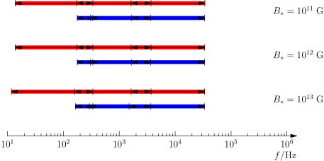
Figure 6: Alfvén (red bands) and cusp (blue bands) continuous frequency spectrum (in Hz) for magnetic mountains with (from top to bottom) polar magnetic field strength $B_{\ast}/\mathrm{G}=10^{13},10^{12},10^{11}$, computed for the node numbers (left bands to right bands) $n=0,10,100$.

We redo the analysis of the previous paragraph, this time varying the polar magnetic field $B_{\ast}$ (Fig. 6). The lower bounds for the Alfvén (cusp) continuum are $\omega_{\mathrm{A,low}}/(2\pi\,\mathrm{Hz})=11.7,13.8,13.8$ [$\omega_{\mathrm{C,low}}/(2\pi\,\mathrm{Hz})=164,177,177$] for $B_{\ast}/\mathrm{G}=10^{11},10^{12},10^{13}$ and $M_{a}=M_{c}$ respectively. The continuous spectrum does not shift much as $B_{\ast}$ varies over two decades. This is not surprising: $M_{c}$ scales as $M_{c}\propto B_{\ast}^{2}$, so that two mountains with a different $B_{\ast}$ but the same $M_{a}/M_{c}$ effectively share the same steady-state hydromagnetic structure and hence the same MHD spectrum.

4.4 Rotational splitting

One expects to find magnetically confined mountains on rapidly rotating neutron stars with $0.1\,\mathrm{kHz}\la\Omega/2\pi\la 0.7\,\mathrm{kHz}$, e.g. in low-mass X-ray binaries, and accreting millisecond pulsars. In such objects, the Coriolis force is an important factor in determining stability. We do not treat the Coriolis force in this article, because our main aim is to compare the analytically derived MHD spectrum with the output from zeus-mp simulations in the literature, which set $\Omega=0$ (Payne & Melatos, 2007; Vigelius & Melatos, 2008c). However, the framework in section 3 and Hellsten & Spies (1979) can easily accomodate $\Omega\neq 0$, as foreshadowed at the end of section 3.1.

Rotation splits the Alfvén and cusp continua, possibly destabilizing them. We perform an order-of-magnitude calculation to estimate the influence of rapid rotation on stability. Note first that the constant term $A$ due to gravitation exceeds its centrifugal counterpart ($A_{\mathrm{1,grav}}\sim GM_{\ast}/R_{\ast}\gg A_{\mathrm{1,rot}}\sim\Omega^{2}R_{\ast}$), justifiying the neglect of the centrifugal force in previous numerical papers (Payne & Melatos, 2007; Vigelius & Melatos, 2008c). For $\Omega\neq 0$, the two equations of (28) couple via the Coriolis force (Hellsten & Spies, 1979):

$$0 = \sigma^{2}NB^{2}Jv^{\theta}-\i 2\sigma\Omega Nr(\mn@boldsymbol{B}\mn@boldsymbol{\cdot}\nabla r)v^{\varphi}+$$ (32)

$$\mn@boldsymbol{B}\mn@boldsymbol{\cdot}\nabla\frac{pB^{2}}{B^{2}+\gamma p}\mn@boldsymbol{B}\mn@boldsymbol{\cdot}\nabla Jv^{\theta},$$

and

$$0=\sigma^{2}Nr^{2}v^{\varphi}+\i 2\sigma\Omega Nr(\mn@boldsymbol{B}\mn@boldsymbol{\cdot}\nabla r)Jv^{\theta}+\mn@boldsymbol{B}\mn@boldsymbol{\cdot}\nabla r^{2}\mn@boldsymbol{B}\mn@boldsymbol{\cdot}\nabla v^{\varphi}.$$ (33)

Clearly, the Coriolis force, which produces the second term in each equation, dominates the other terms. For (32), we find $|[2\sigma\Omega Nr(\mn@boldsymbol{B}\mn@boldsymbol{\cdot}\nabla r)]/(\sigma^{2}NB)|\sim\Omega/\sigma=10^{2}\gg 1$, and for the third term $|[2\sigma\Omega Nr(\mn@boldsymbol{B}\mn@boldsymbol{\cdot}\nabla r)]/[\mn@boldsymbol{B}\mn@boldsymbol{\cdot}\nabla(NB^{2})(B^{2}+\gamma p)\mn@boldsymbol{B}\mn@boldsymbol{\cdot}\nabla J]|\sim(\sigma\Omega\eta^{2})/c_{s}^{2}=10^{6}\gg 1$. Equivalently, for (33), we find $|[2\sigma\Omega Nr(\mn@boldsymbol{B}\mn@boldsymbol{\cdot}\nabla rJ)]/(\sigma^{2}Nr^{2})|\sim\Omega/\sigma=10^{2}\gg 1$, and $|[2\sigma\Omega Nr(\mn@boldsymbol{B}\mn@boldsymbol{\cdot}\nabla rJ)]/(\mn@boldsymbol{B}\mn@boldsymbol{\cdot}\nabla r^{2}\mn@boldsymbol{B}\mn@boldsymbol{\cdot}\nabla)|\sim\sigma\Omega N/B^{2}=10^{6}\gg 1$. A more general analysis including rotation is therefore needed in the future.

5 Discussion

In this article, we compute semi-analytically the continuous part of the ideal-MHD frequency spectrum of axisymmetric, magnetically confined mountains. We find that the continuous spectrum covers all frequencies above a minimum $\omega_{\mathrm{min}}$. Furthermore, we find $\omega^{2}_{\mathrm{min}}>0$ in all the configurations ($0.01\leq M_{a}/M_{c}\leq 1.4$) we study. This further substantiates two important properties deduced previously from numerical simulations: (i) magnetic mountains are marginally stable, i.e., $\omega$ has zero imaginary part; and (ii) mountains relax hydromagnetically through the undulating submode of the three-dimensional Parker instability (Vigelius & Melatos, 2008c), which possesses discrete eigenvalues only. We also find that, for $M_{a}\ga M_{c}$, when the magnetic structure of the mountain substantially deviates from a dipole, $\omega_{\mathrm{min}}$ for the Alfvén and cusp continua depends weakly on $M_{a}$ and $B_{\ast}$.

Figure 7: Fourier transform $\epsilon(f)$ of the mass ellipticity taken from zeus-mp simulations of magnetic mountains with $M_{a}=M_{c}$ (solid), $M_{a}=1.4M_{c}$ (dotted), and $M_{a}=0.6M_{c}$ (dashed). The continuous Alfvén spectrum is clearly visible for $M_{a}=M_{c}$ as a band starting at $\approx 11$ Hz. We mark the theoretical analytic values of $f_{\mathrm{A,low}}=11.1,16,14\;\mathrm{Hz}$ for $M_{a}/M_{c}=0.6,1,1.4$, respectively, as vertical lines. Note that the cusp continuum, with $\omega_{\mathrm{C,low}}=177.07$ Hz, lies outside the range of this plot, since it exceeds the Nyquist limiting frequency $\omega_{\mathrm{N}}=44.5$ Hz.

How do our analytic results compare with numerical simulations of oscillating magnetic mountains (Payne & Melatos, 2007; Vigelius & Melatos, 2008c)? To answer this question, we perform an axisymmetric ideal-MHD simulation of a magnetic mountain with $M_{a}=M_{c}$, which is perturbed slightly at $t=0$. The simulation is performed using the parallel ideal-MHD solver zeus-mp (Hayes et al., 2006). Fig. 7 shows the Fourier transform $\epsilon(f)$ of the mass ellipticity $\epsilon(t)$, which is proportional to the mass quadrupole moment of the mountain [see Eq. (2) in Vigelius & Melatos (2008c)]. We choose $\epsilon$ to compute the spectrum as (i) it is directly measurable from future gravitational wave data (Vigelius & Melatos, 2008a) and (ii) it is an integrated quantity sampling $N$ and $\mn@boldsymbol{B}$ everywhere, so it is sensitive to all global oscillation modes.

Besides the constant offset at $f=0$, the simulation with $M_{a}=M_{c}$ (solid curve in Fig. 7) exhibits a continuous spectrum with a lower boundary at $f\approx 11\;\mathrm{Hz}$. This is consistent with the analytic theory in section 4, which yields $f_{\mathrm{A,low}}=16\;\mathrm{Hz}$, indicated as a vertical line in Fig. 7. The width of a frequency bin is $\delta f=1.45$ Hz, so we conclude that the lower boundary of the simulated spectrum almost coincides with $f_{\mathrm{A,low}}$. It appears that the lowest modes of the continuous Alfvén spectrum are indeed excited in zeus-mp simulations, substantiating the claim that global MHD mountain oscillations are Alfvénic (Payne & Melatos, 2007). For $M_{a}=1.4M_{c}$ (dotted curve in Fig. 7), we see a continuous spectrum at $f\ga 7$ Hz, albeit less distinctly than in the $M_{a}=M_{c}$ case. The $M_{a}=0.6M_{c}$ simulation (dashed) shows a peak at $f=23$ Hz and no obvious continuous spectrum.

We do not attempt a unambiguous identification of the oscillation modes seen in the above simulation. As an integrated quantity, the behaviour of $\epsilon$ is determined by a global superposition of different eigenmodes, both, continuous and discrete. These eigenmodes are stochastically excited through numerical inaccuracies (Vigelius & Melatos, 2008c) in the simulation displayed in Fig. 7 and identifying the frequency spectrum of $\epsilon$ with the underlying eigenfunctions is hence difficult. The calculations undertaken in this article are but a first step towards a thorough investigation of the complete eigenvalue problem.

In the context of future gravitational wave observations of magnetic mountains in low-mass X-ray binaries (Melatos & Payne, 2005), the MHD oscillation spectrum enters the gravitational wave signal through sidebands and broadening near the Fourier peaks at $f_{\ast}$ and $2f_{\ast}$, where $f_{\ast}$ is the spin frequency of the neutron star. Vigelius & Melatos (2008a) showed that the sidebands can be observed in principle with next-generation interferometers. However, in order to exploit these features fully to probe the physics of surface magnetic fields on accreting neutron stars, we need to know more about how the oscillations are excited (e.g. by the variable accretion torque) and damped. The analytic technique in this article is a useful tool for such investigations.

The oscillation modes may be perpetually re-excited, e.g. through starquakes, variable accretion torques (Lai, 1999), and possibly cyclonic flows during type I X-ray bursts (Spitkovsky et al., 2002). Vigelius & Melatos (2008a) show that a perturbation of the fluid density causes a fractional change in the signal-to-noise ratio $d$ of $\delta d/d\approx n/N$. Similarly, in a (very crude) model where the pulse shape is determined by the positions of the footpoints of the magnetic field lines at the polar cap boundary, the fractional change in pulse parameters (e.g. full-width half-maximum) is comparable to the fractional perturbation amplitude. Unfortunately, the excitation mechanisms are poorly understood and it is unclear if the amplitude of the perturbation is sufficient to cause observable features in the gravitational wave spectrum. Ultimately, gravitational wave observations will yield valuable information about the underlying excitation physics.

Glampedakis et al. (2007) investigated ideal-MHD modes in magnetars, taking into account the coupling between the fluid core and the elastic crust. They found that global core-crust modes can explain quasi-periodic oscillations (QPOs) observed during giant flares in the soft gamma-ray repeaters SGR 1806$-$20 and SGR 1900$+$14. In contrast, Levin (2006) argued that continuous coupled modes in magnetars decay too rapidly to account for the observed QPOs. This debate was reviewed recently by Watts & Strohmayer (2007). Using a series expansion, Lee (2007, 2008) calculated the discrete eigenmodes of magnetars. While low frequency QPOs can be identified with fundamental toroidal torsional modes, higher frequency ($100\la f\la 1000$ Hz) can be attributed to a variety of modes, such as spheroidal shear modes or core/crust interfacial modes.

The aim of this paper is to interprete analytically and physically the magnetic mountain oscillations seen in nonrotating numerical simulations (Payne & Melatos, 2007; Vigelius & Melatos, 2008a). For rapidly rotating objects with $\Omega/2\pi\ga 0.1$ kHz, like accreting millisecond pulsars, the continuous spectrum is strongly modified by rotation, as shown in section 4.4. We will calculate the rotational splitting in a forthcoming paper.

References

- Bisnovatyi-Kogan & Komberg (1974) Bisnovatyi-Kogan G. S., Komberg B. V., 1974, Soviet Astronomy, 18, 217
- Brown & Bildsten (1998) Brown E. F., Bildsten L., 1998, ApJ, 496, 915
- Choudhuri & Konar (2002) Choudhuri A. R., Konar S., 2002, MNRAS, 332, 933
- Glampedakis et al. (2007) Glampedakis K., Samuelsson L., Andersson N., 2007, Ap&SS, 308, 607
- Goedbloed & Poedts (2004) Goedbloed J. P. H., Poedts S., 2004, Principles of Magnetohydrodynamics. Cambridge University Press, Cambridge.
- Hartman et al. (2008) Hartman J. M., Patruno A., Chakrabarty D., Kaplan D. L., Markwardt C. B., Morgan E. H., Ray P. S., van der Klis M., Wijnands R., 2008, ApJ, 675, 1468
- Hayes et al. (2006) Hayes J. C., Norman M. L., Fiedler R. A., Bordner J. O., Li P. S., Clark S. E., ud-Doula A., Mac Low M.-M., 2006, ApJS, 165, 188
- Hellsten & Spies (1979) Hellsten T. A. K., Spies G. O., 1979, Physics of Fluids, 22, 743
- Konar & Bhattacharya (1997) Konar S., Bhattacharya D., 1997, MNRAS, 284, 311
- Lai (1999) Lai D., 1999, ApJ, 524, 1030
- Lee (2007) Lee U., 2007, MNRAS, 374, 1015
- Lee (2008) Lee U., 2008, MNRAS, 385, 2069
- Levin (2006) Levin Y., 2006, MNRAS, 368, L35
- Lifschitz (1989) Lifschitz A. E., 1989, Magnetohydrodynamics and Spectral Theory. Kluwer Academic Publishers, London.
- Litwin et al. (2001) Litwin C., Brown E. F., Rosner R., 2001, ApJ, 553, 788
- Lovelace et al. (2005) Lovelace R. V. E., Romanova M. M., Bisnovatyi-Kogan G. S., 2005, ApJ, 625, 957
- Melatos & Payne (2005) Melatos A., Payne D. J. B., 2005, ApJ, 623, 1044
- Melatos & Phinney (2001) Melatos A., Phinney E. S., 2001, Publ. Astronom. Soc. Aust., 18, 421
- Mouschovias (1974) Mouschovias T. C., 1974, ApJ, 192, 37
- Muno et al. (2002) Muno M. P., Özel F., Chakrabarty D., 2002, ApJ, 581, 550
- Parker (1967) Parker E. N., 1967, ApJ, 149, 535
- Payne & Melatos (2004) Payne D. J. B., Melatos A., 2004, MNRAS, 351, 569
- Payne & Melatos (2006) Payne D. J. B., Melatos A., 2006, ApJ, 641, 471
- Payne & Melatos (2007) Payne D. J. B., Melatos A., 2007, MNRAS, 376, 609
- Press et al. (1986) Press W. H., Flannery B. P., Teukolsky S. A., 1986, Numerical recipes. The art of scientific computing. Cambridge: University Press, 1986
- Romani (1990) Romani R. W., 1990, Nature, 347, 741
- Spitkovsky et al. (2002) Spitkovsky A., Levin Y., Ushomirsky G., 2002, ApJ, 566, 1018
- Taam & van de Heuvel (1986) Taam R. E., van de Heuvel E. P. J., 1986, ApJ, 305, 235
- van den Heuvel & Bitzaraki (1995) van den Heuvel E. P. J., Bitzaraki O., 1995, A&A, 297, L41+
- Vigelius & Melatos (2008a) Vigelius M., Melatos A., 2008a, MNRAS(submitted)
- Vigelius & Melatos (2008b) Vigelius M., Melatos A., 2008b, MNRAS(submitted)
- Vigelius & Melatos (2008c) Vigelius M., Melatos A., 2008c, MNRAS, 386, 1294
- Watts et al. (2008) Watts A., Krishnan B., Bildsten L., Schutz B., 2008, preprint (astro-ph/0803.4097)
- Watts & Strohmayer (2007) Watts A. L., Strohmayer T. E., 2007, Advances in Space Research, 40, 1446
- Zhang (1998) Zhang C. M., 1998, Ap&SS, 262, 97