Spontaneous Emergence of Modularity in a Model of Evolving Individuals and in Real Networks

Abstract

We investigate the selective forces that promote the emergence of modularity in nature. We demonstrate the spontaneous emergence of modularity in a population of individuals that evolve in a changing environment. We show that the level of modularity correlates with the rapidity and severity of environmental change. The modularity arises as a synergistic response to the noise in the environment in the presence of horizontal gene transfer. We suggest that the hierarchical structure observed in the natural world may be a broken symmetry state, which generically results from evolution in a changing environment. To support our results, we analyze experimental protein interaction data and show that protein interaction networks became increasingly modular as evolution proceeded over the last four billion years. We also discuss a method to determine the divergence time of a protein.

I introduction

Modularity abounds in biology. Elements of hierarchy—modules—are found in developmental biology, evolutionary biology, and ecology Shapiro (2004, 2005); Misevic et al. (2006). Modularity is observed at levels that span molecules, cells, tissues, organs, organisms, and societies. At the genomic level, there are introns, exons, chromosomes, and genes. Moreover, there are mechanisms to rearrange and transmit the information that is modularly encoded at the genomic level, such as gene duplication, transposition, and horizontal gene transfer Shapiro (1992); Goldenfeld and Woese (2007). We define a module to be a component that can operate relatively independently of the rest of the system. From a structural perspective, existence of modularity means there are more intra-module connections than inter-module connections. From a functional perspective, a module is a unit that can perform largely the same function in different contexts. Modularity has been characterized in a variety of network systems by physical methods Lipson et al. (2002); Tanase-Nicola et al. (2006). Selection for stability, for example, has been shown to select for modular networks Variano et al. (2004). A dictionary of constituent parts, or network motifs, has been identified for the transcriptional regulation network of E. coli Shen-Orr et al. (2002). And once modularity has arisen, so that the goals a species face become modular, modularly varying goals have been shown to select for modular structure Kashtan and Alon (2005). Horizontal gene transfer has been suggested to be essential to the evolution of a universal genetic code Vetsigian et al. (2006).

How does modularity arise in nature? It has been suggested that by being modular, a system will tend to be both more robust to perturbations and more evolvable Csete and Doyle (2002); Kitano (2004); Oikonomou and Cluzel (2006). It has further been suggested that there is a selective pressure for positive evolvability in a population of individuals in a changing environment Earl and Deem (2004). Thus, we have hypothesized that modularity arises spontaneously from the generic requirement that a population of individuals in a changing environment be evolvable Deem (2007). Support for this hypothesis had been elusive Gardener and Zuidema (2003).

In this article, we extend the analysis presented in Sun and Deem (2007), as well as discuss experimental data. In Section II, we introduce the spin glass model for the replication rate in evolution. In Section III, we show spontaneous evolution of hierarchy in a system under changing environmental conditions with horizontal gene transfer. Specifically, we show that in the presence of horizontal gene transfer, environmental change leads to the spontaneous emergence of modularity in a generic model of a population of evolving individuals. The model describes evolution in a rugged landscape, when the environment is changing and when horizontal gene transfer is possible. Modularity grows spontaneously even when the horizontal gene transfer event is of a random length and starting location. In Section IV, we discuss experimental evidence in support of our simulation results. First we review the evidence showing that the bacterial metabolic networks in more variable environments are more modular. Next, we show using a measure of protein divergence time that modularity in protein interaction networks and protein domain interaction networks appears to have increased with time. We conclude in Section V. Additional details are presented in Appendices.

II spin glass model of evolution

To represent the replication rate, or microscopic fitness, of the individuals, we use a spin glass model that has proved useful in previous studies of evolution Kauffman and Levin (1987); Deem and Lee (2003); Sun et al. (2005). The choice of a spin glass model, with many local fitness optima, is motivated by our assumption that evolution occurs on a rugged landscape. In other words, our results pertain only to those evolutionary processes that occur on such rugged fitness landscapes. A spin glass model generically represents such rugged fitness landscapes. We present illustrative results for some numerical values of the parameters in the model. The qualitative nature of our results are insensitive to the specific values of these parameters. In this model, spontaneous emergence of modularity, however, generically occurs for a population of evolving individuals and depends only on the presence of a changing environment and the presence of horizontal gene transfer. This spin glass model is appropriate because it provides a rugged, difficult landscape upon which evolution struggles to occur, and so there can be a pressure for more efficient evolutionary structures to arise. This rugged landscape of this model is expected to reproduce the slow dynamics of evolution Anderson (1983); Stein and Anderson (1984); Kauffman and Levin (1987); Perelson and Macken (1995); Mezard et al. (1987), and we have used correlated random energy models in a number of protein evolution Bogarad and Deem (1999); Earl and Deem (2004) and immune system evolution studies Deem and Lee (2003); Sun et al. (2005, 2006). There are three time scales in our system: the fastest time scale of sequence evolution of population as descendants replace parents, the intermediate time scale of environmental change, and the longest time scale of the change to the structure of interactions between elements of the sequence space. The symmetry of a uniformly random structure is broken by the spontaneous emergence of modular structure as a response to environmental change.

We use the following spin glass form for the microscopic fitness of proteins in our system (for a discussion on the spin glass approach to evolution, see Deem and Lee (2003); Earl and Deem (2004); Sun et al. (2005, 2006)):

$$H^{\alpha}(s^{\alpha,l})=\frac{1}{2\sqrt{N_{D}}}\sum_{i\neq j}\sigma_{i,j}(s^{\alpha,l}_{i},s^{\alpha,l}_{j})\cdot\Delta_{i,j}^{\alpha},$$ (1)

where $s^{\alpha,l}_{i}$, $1\leq i\leq N$, is a string of length $N$ that specifies the identity of “individual” $l$. The term $s^{\alpha,l}_{i}$ may represent the amino acid at position $i$ within the sequence of a protein, the label of a protein at gene $i$ in the genome, or the type of transcriptional regulatory element at non-coding position $i$. For these three examples, the modularity that may develop represents the formation of secondary structure, protein-protein interaction motifs, or regulatory structure, respectively. The different individuals are enumerated by $l$, with $1\leq l\leq N_{\rm size}$, where we have $N_{\rm size}$ different individuals. The different possible forms of the structure of the interaction between the $s^{\alpha,l}_{i}$ are enumerated by $\alpha$, $1\leq\alpha\leq D_{\rm size}$, where we choose $D_{\rm size}$ possible structures. These structures of the interaction represent, for example, the protein fold, protein interaction pathways, or constraints on regulation. The term $\sigma_{i,j}(s_{i},s_{j})$, is the numerical value of the interaction matrix, symmetric in $i$ and $j$, whose elements are each taken from a Gaussian distribution with zero mean and unit variance. It differs for each $i$, $j$, $s_{i}$, and $s_{j}$. The effect of the environment is encoded by these random couplings. When the environment changes with severity $p$, each of the couplings is with probability $p$ randomly redrawn from the Gaussian distribution. The term $\Delta_{i,j}^{\alpha}$ defines the structure of the interaction, i.e. the contact matrix, or connections in structure, for structure $\alpha$. The matrix is symmetric, with elements 0 or 1. In order to guarantee that the emergence of modularity comes from redistribution of connections rather than an increase in the number of connections, we constrain $\sum_{i>j+1}\Delta_{i,j}^{\alpha}=N_{D}=346$. Any value of $N_{D}$ such that the connection matrix is neither all unity nor all zero would give qualitatively similar results. We take $\Delta_{i,i}^{\alpha}=0$ and $\Delta_{i,i\pm 1}^{\alpha}=1$.

Horizontal gene transfer is assumed, for specificity, to transfer any of the 12 blocks of length 10 in the sequence (i.e. sequence elements 1 …10, 11 …20, 21 …30, etc.). This horizontal gene transfer event represents transfer of pieces of genes, collections of genes, or stretches of non-coding regulatory information between individuals. Modularity is defined, conjugate to the horizontal gene transfer event, to be the number of connections within the 12 $10\times 10$ blocks along the diagonal

$$M^{\alpha}=\sum_{k=0}^{11}\sum_{i=1,j=i+2}^{10}\Delta_{10k+i,10k+j}^{\alpha},$$ (2)

so that $i,j$ are within the $1+k^{th}$ diagonal block of size $10$. Even a random distribution of contacts will have a non-zero absolute modularity, $M_{0}$, and so it is the excess modularity that measures the degree of spontaneous symmetry breaking, $\delta M^{\alpha}=M^{\alpha}-M_{0}$. Emergence of modularity means that as a result of evolution, connections in structure are not evenly distributed between positions. The interactions are greater in the local, diagonal blocks than in the rest of the matrix, and so $\delta M^{\alpha}>0$. In other words, $\delta M^{\alpha}$ is the order parameter of spontaneous symmetry breaking of the approximately uniform distribution of contacts, and in the broken symmetry phase, where the distribution of contacts is not uniform, and $\delta M^{\alpha}\neq 0$.

In order to see the emergence of modularity, we need a set of individuals in a changing environment. Moreover, since we want to watch the evolution of the structural connections $\Delta_{i,j}^{\alpha}$, we need a population of these sets, each set with a different $\Delta_{i,j}^{\alpha}$. We take the population size to be $D_{\rm size}=300$ different structures, $1\leq\alpha\leq D_{\rm size}$, and each given structure has a set of $N_{\rm size}=1000$ different sequences, $1\leq l\leq N_{\rm size}$, associated with them. In total there are $D_{\rm size}\times N_{\rm size}=3\cdot 10^{5}$ different individuals, replicating at the rate given by the microscopic fitness associated with its set [see Eq. (3), below]. The average excess modularity is given by $\delta M=M-M_{0}=\frac{1}{D_{\rm size}}\sum_{\alpha=1}^{D_{\rm size}}M^{\alpha}-M_{0}$.

The structures, $\Delta_{i,j}^{\alpha}$, are initialized by first randomly generating one such structure with $N_{D}=346$ and a certain $M$. We then obtain the full set of $D_{\rm size}$ structures by evolution away from this structure. Two elements of $\Delta_{i,j}^{\alpha}$ with opposite status are randomly chosen, and the status of each is flipped from $1\to 0,0\to 1$. These mutations are done $n$ times, where $n$ is a Poisson random number with mean 2. The sequences, $s^{\alpha,l}_{i},1\leq i\leq N$, of each individual are initialized by random assignment.

The evolution in our simulation involves three levels of change. The most rapid change occurs by evolution of the sequences through mutation and horizontal gene transfer. The selection on this level is based on the microscopic fitness. For each structure $\Delta_{i,j}^{\alpha}$, at each round, all the $N_{\rm size}$ associated sequences undergo mutation, horizontal gene transfer, and selection. The Poisson mutation process changes on average $2.4$ values of the $s^{\alpha,l}_{i}$ in the sequence, which are randomly selected and assigned a random new value. In horizontal gene transfer, two randomly selected sequences from the population associated with one structure attempt to exchange each of the 12 sequence fragments between $10k+1$ and $10k+10$ (of length $10$) with probability $0.1$. Thus, the horizontal gene transfer rate and the mutation rate are roughly equal Park and Deem (2007). The qualitative behavior of the results does not depend on the exact mutation rates. All the sequences undergo attempted horizontal gene transfer to make the new population. Pairs of sequences in the population associated with one structure are chosen, until all sequences have been chosen. This process is a model of horizontal gene transfer or recombination. The 50% sequences with the lowest energy are selected and randomly duplicated to recover the population of $N_{\rm size}$ for the next round; the microscopic replication rate, or fitness, for sequence $\alpha,l$ in structure $\alpha$ is

$$r^{\alpha}(s^{\alpha,l})=2\theta[H^{\alpha}_{{\rm N_{size}}/2}-H^{\alpha}(s^{\alpha,l})]\ ,$$ (3)

where $\theta(x)$ is the Heavyside step function. Mutation and selection are repeated $T_{2}$ rounds.

The next most rapid change is that of the environment, which occurs with severity $p$ and frequency $1/T_{2}$. That is, the set of individuals evolve for $T_{2}$ rounds in each given environment, and then the environment changes. During the environmental change, the elements of the interaction matrix $\sigma_{i,j}$ change with probability $p$.

The slowest level of change is the structural evolution. The selection at this level is based on the cumulative fitness of the set of individuals with a given structure, averaged over $T_{3}=10^{4}T_{2}$ environmental changes. That is, we sum the average energy of the sequence set of each structure at the end of each environment for $T_{3}/T_{2}$ times and use this cumulative fitness to determine the replication rate of the structures, quantifying their performance in responding to environment changes. The structures with the best $5\%$ cumulative fitness are selected and randomly amplified to make the new population of $D_{\rm size}$ structures, $\Delta^{\alpha}_{ij}$. The structure population also undergoes mutation. As with the initial construction, two elements of $\Delta_{i,j}^{\alpha}$ with opposite status are randomly chosen, and the status of each is flipped from $1\to 0,0\to 1$. These mutations are done $n$ times, where $n$ is a Poisson random number with mean 2. The mutated structures, $\Delta_{i,j}^{\alpha}$, are used for the next $T_{3}$ rounds of evolution.

III spontaneous emergence of modularity

In Fig. 1, we show the spontaneous emergence of modularity from the symmetric, random state of no excess modularity, $M=M_{0}=22$. Since the system is initially quite far from the steady state modularity, the growth of the excess modularity with time is roughly linear. The excess modularity is the order parameter for this system, and its growth shows that the system is in a broken symmetry phase with modular structure under these conditions. In Fig. 2, we show the energy decreases as modularity grows, i.e. the stability of the structure is increasing. In Fig. 3, we show the change of energy with time in more detail. Compared with Fig. 2, the time scale ($x$-axis) in Fig. 3 is much smaller ($T_{3}=2\times 10^{5}$). The energy decreases during each constant environment. The environment changes each $t=20$ steps. Immediately after the change of environment, the individual sequences are not as well adapted, and so the the energy increases sharply. As the sequences adapt in the new environment, the average energy of the population decreases. In Fig. 4, the response function, or evolvability, $\Delta$E, is shown as a function of time. By evolvability, we mean the rate of change in a new environment Earl and Deem (2004). We observed the growth of evolvability as the modularity grows in Figs. 5 and 4.

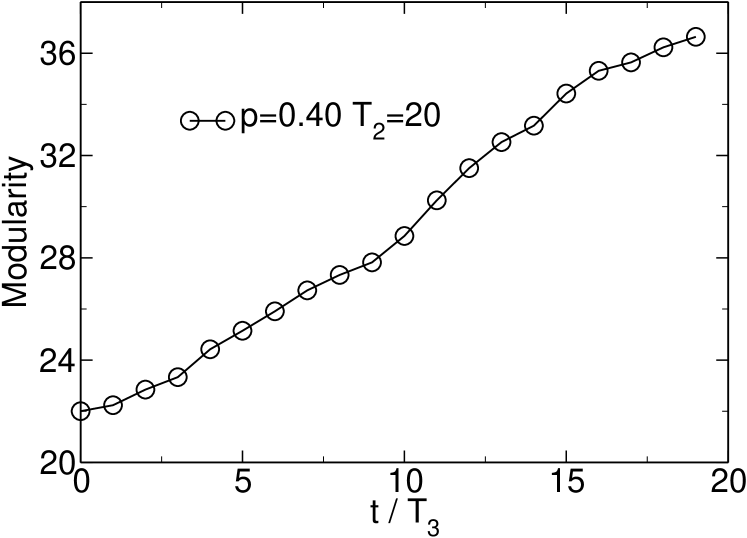
Figure 1: Spontaneous emergence of excess modularity, $M>M_{0}=22$, from a state with no excess modularity, $M=M_{0}$. The random, symmetric distribution of structural connections is spontaneously broken as the system evolves. Here $T_{2}=20$, $T_{3}=10^{4}\times T_{2}$, and the severity of environmental change is $p=0.40$.

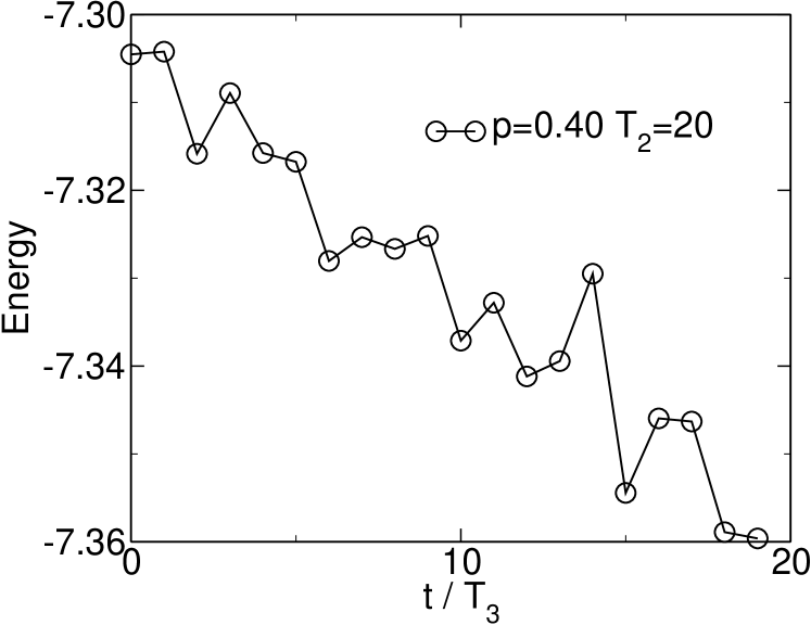
Figure 2: Improvement in the energy as time increases and as the modularity grows, as shown by Fig. 1. Here the severity of environmental change is $p=0.4$, and the period of change is $T_{2}=20$. Here, and in all figures, $T_{3}=10^{4}\times T_{2}$.

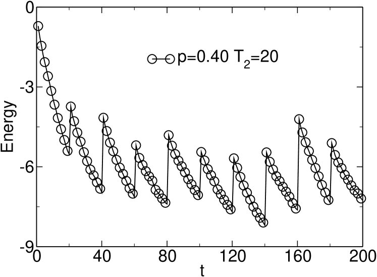
Figure 3: Energy improvement as evolution proceeds within each environment and large energy disruption due to environmental changes. Here the severity of environmental change is $p=0.4$, and the period of change is $T_{2}=20$.

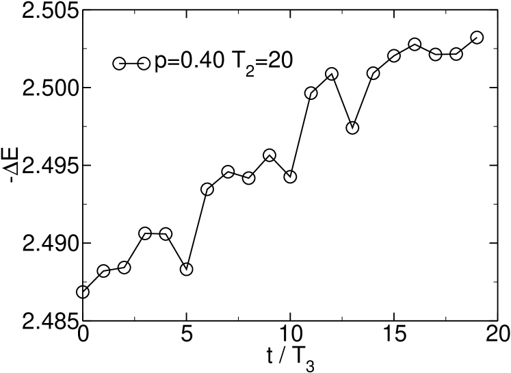
Figure 4: Improvement of evolvability, or evolved improvement of the energy in one environment, as the modularity grows. Here the severity of environmental change is $p=0.4$, and the period of change is $T_{2}=20$.

Interestingly, the growth of modularity is identical for an initial contact matrix that is power-law distributed. Many biological networks appear scale free, at least over a limited range of connectivity Barabási and Oltvai (2004), with a power-law degree distribution. Here, we choose the Barabási et al.’ method Barabási and Oltvai (2004) to generate an initial contact matrix that is power-law distributed with $\gamma=3$. In Fig. 5, we show the growth of modularity that is nearly identical to that of Fig. 1.

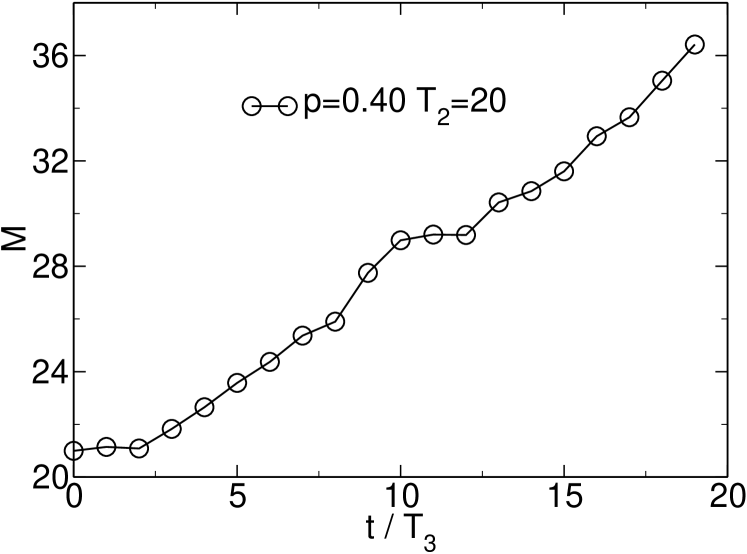
Figure 5: Spontaneous emergence of excess modularity, $M>M_{0}=22$, from an initial scale-free network ($\gamma=3$) with $M=M_{0}$. Here $T_{2}=20$, and the severity of environmental change is $p=0.40$.

The spontaneous emergence of modularity is a general result. In Fig. 6, we show the excess modularity still grows, even if the gene transfer starts at a uniformly random position and swaps a random length of sequence. the original assumption of fixed length and position, however, is biologically motivated. If we take the specific instance of the model to indicate formation of secondary structures or protein-protein interactions, then if the blocks are exons, and the ratio of non-coding to coding DNA is large, then typical recombination or horizontal gene transfer will transfer an integer number of complete exons, which is our horizontal gene transfer operator of fixed length and position.

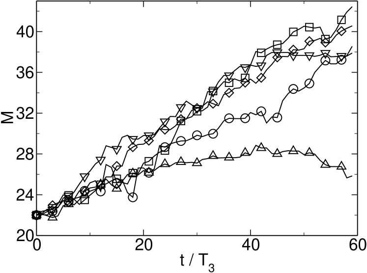
Figure 6: Emergence of modularity as a result of a horizontal gene transfer operator with a Poisson random swap length and uniform random starting position. Shown are data for an average swap length of 10 ($\bigcirc$), 20 ($\Box$), 20 ($\Diamond$), 5 ($\bigtriangleup$), and 40 ($\bigtriangledown$) with 12, 6, 12, 24, and 3 attempted swaps, respectively, of probability 0.1 per sequence pair. Here $T_{2}=20$, and the severity of environmental change is $p=0.40$.

When the environment does not change, or if there is no horizontal gene transfer, the modularity does not spontaneously emerge. As shown in Fig. 7, the modularity remains constant at $M_{0}$ without environmental change or gene transfer.

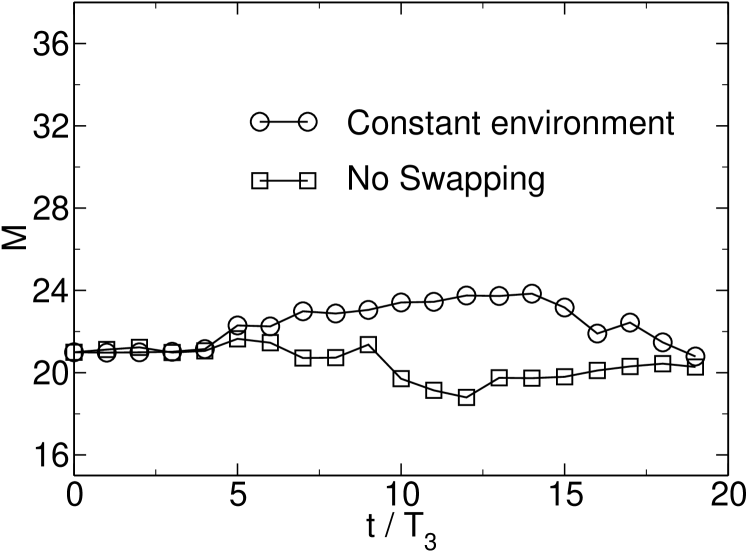
Figure 7: Emergence of modularity in this model requires both horizontal gene transfer and a changing environment. Here $T_{2}=20$. For the case of no horizontal gene transfer with a changing environment, the severity of environmental change is $p=0.40$. For the case of no environmental change with horizontal gene transfer, $p=0$, and the transfer is of fixed position $10k+1$ and fixed length 10 and attempted every $T_{2}$ steps.

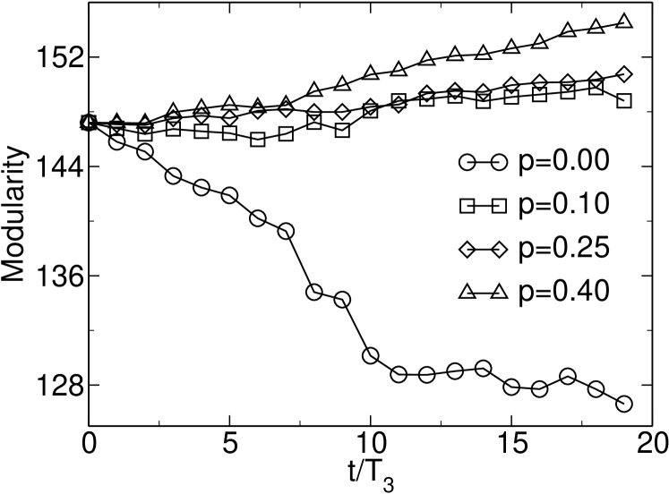
Figure 8: The rate at which modularity grows, $dM/dt$, is positively correlated with the magnitude of environment change, $p$. The frequency of environment change is set at $1/T_{2}=1/40$.

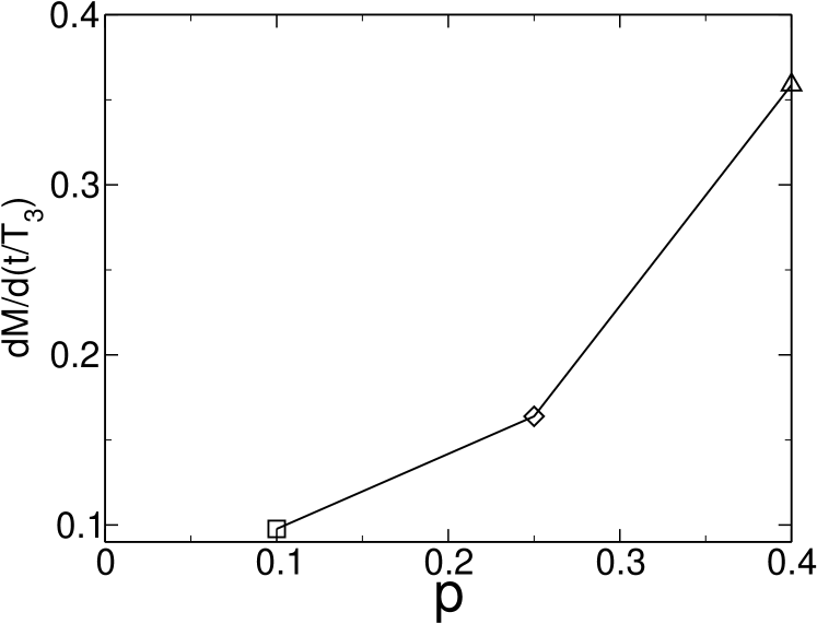
Figure 9: The response function of the system, $dM/d(t/T_{3})$, as a function of the severity of environmental change for the data of Fig. 8.

The system adopts the broken-symmetry, modular state not because the mutation and horizontal gene transfer moves favor modularity a priori, but rather because these moves enable the system to respond more effectively to a changing environment when the system is modular. That is, evolvability is implicitly selected for in a changing environment, and horizontal gene transfer enhances evolvability if the system is modular. Thus, we expect modularity to be implicitly selected for in a changing environment in the presence of horizontal gene transfer, with the degree of modularity positively correlated to the degree of environmental change. In Fig. 8 we show the change of modularity with time for different severities of environmental change, $p$. For this figure, we choose the initial set of structures from an ensemble with $M=147$, rather than $M=M_{0}$, to show the change of modularity more clearly. For no environmental change, the modularity decreases from this high level. But for modest environmental change, the modularity increases from the initial, high level. When the environment changes greatly, the system must carry out more genetic change to survive, and it evolves a greater increase of modularity. In Fig. 9, $dM/d(t/T_{3})$ is the rate of the increase of modularity, and we show that the rate of the increase of modularity is larger for greater environmental change.

Another way of characterizing the environmental change is by the frequency of change, and the emergence of modularity depends on this parameter as well. In Fig. 10 we show the growth of modularity with time for different frequencies of environmental change. For frequencies of environmental change that are not too large, the modularity increases with frequency. For very high frequencies, $1/T_{2}>1/5$, the system is unable to track the changes in the environment, and the modularity decays with frequency. Fig. 11 is the same as Fig. 10 but with a real time as the $x$-axis. We can see that the increase of modularity is almost linear. The rate of modularity increase in Fig. 10 for $p=0.40$ and $T_{2}=20$ is less than that in Fig. 1 because in Fig. 10 the system is closer to the steady-state, broken-symmetry value than it is in the Fig. 1. In Fig. 12, we show that the rate of the increase of modularity is larger for higher frequencies of environmental change.

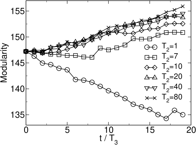
Figure 10: Frequency of environmental change also affects the time evolution of spontaneous modularity. Here $1/T_{2}$ is the frequency of environmental change, and the severity of environment change is $p=0.40$.

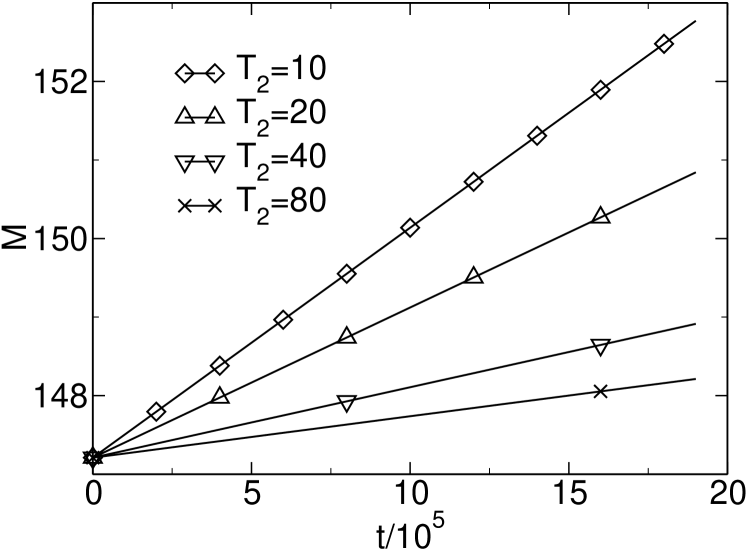
Figure 11: Frequency of environmental change affects the time evolution of spontaneous modularity shown in real time, $t$. Here $1/T_{2}$ is the frequency of environmental change, and the severity of environment change is $p=0.40$.

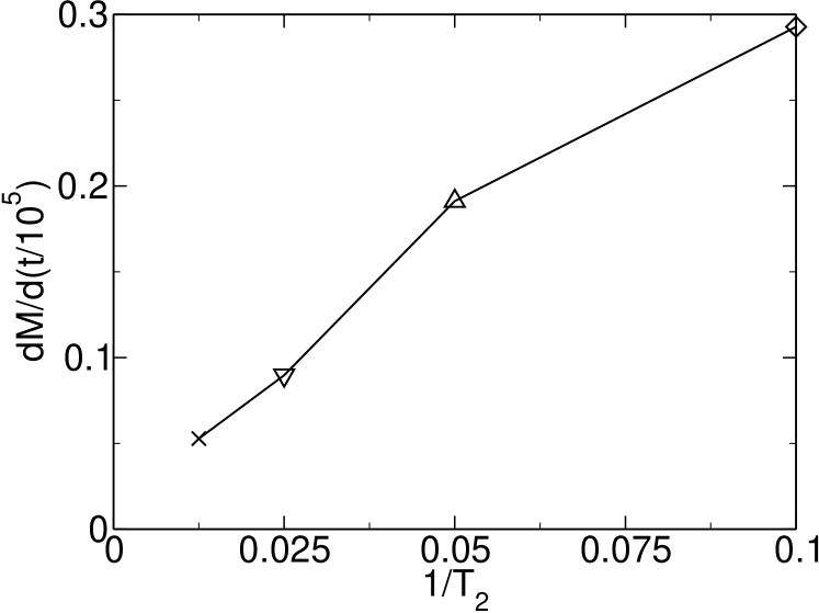
Figure 12: The response function of the system $dM/d(t/10^{5})$ as a function of the frequency of environmental change ($1/T_{2}$) for the data from Fig. 10.

The spontaneous emergence of modularity is caused by the historical variation in environments that the system has encountered. By a fluctuation-dissipation argument Gammaitoni et al. (1998); Sato et al. (2003); Earl and Deem (2004), we might expect that the degree of modularity should be proportional to the variance of environments encountered. In Fig. 9 we show that the rate of the increase in modularity is roughly proportional to the severity of environmental change, $p$. In Fig. 12 we show that the rate of the increase in modularity is roughly proportional to the frequency of environmental change, $1/T_{2}$.

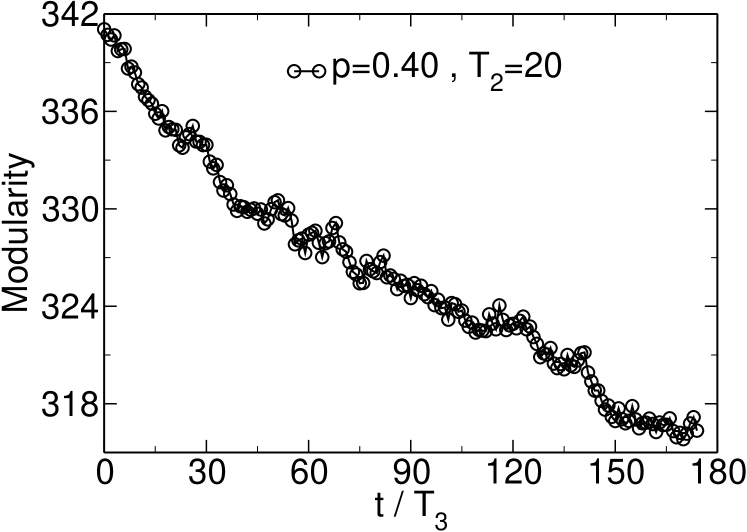
Figure 13: The spontaneous modularity saturates at a steady-state level. If the initial value of the modularity is greater than the steady-state value, the modularity decays with time. Here $T_{2}=20$, and the severity of environment change is $p=0.40$.

While the modularity grows with time in Figs. 1, 8, and 10 for $p>0$ and $T_{2}>5$, at steady state the system will be only partially modular, $M<N_{D}=346$, reflecting a balance between the selection for modularity in a changing environment and the mutations driving the system toward the symmetric state of no excess modularity. To illustrate this point of a finite modularity in the steady state, we show in Fig. 13 how the modularity changes from a starting point of nearly total modularity, $M\approx N_{D}$, i.e. nearly all the connections in the diagonal blocks and few in the off-diagonal blocks. We observe that the modularity decays from the initial value. See Fig. 13. The excess modularity in the broken symmetry state is positive because of selection for modularity in fluctuating environments, and the excess modularity is not the maximal possible value of $M=N_{D}=346$ because of the entropic effects of the mutations in the sequence space. For the initial condition used in Fig. 13, nearly all the connections in the diagonal blocks and few in the off-diagonal blocks, modularity decays over time, showing the steady state value is below $316$. The modularity will saturate at a value for which the effects of selection pressure and mutation balance each other.

To summarize, we have observed the spontaneous evolution of modularity in a population evolving in a changing environment. While we have described the model parameters in terms of an evolving population of proteins, the model generically represents evolution of individuals in a population with a non-trivial microscopic fitness landscape. Modularity arises spontaneously because evolvability is selected for in a changing environment Earl and Deem (2004), and modularity allows the horizontal gene transfer to rapidly evolve the system in a modified environment. Thus, modularity is selected for in a changing environment, when the system has access to horizontal gene transfer. The rate at which modularity grows with time depends on the amplitude and frequency of environment changes. More rapid environmental change tends to promote the growth of modularity. A constant environment promotes no emergence of modularity, as does the limit of an extremely rapidly varying environments, because the system sees only the average, constant environment. The growth of modularity is also accelerated by more severe, larger-amplitude environmental changes.

IV discussion

In this section, we present some experimental evidence in support of our simulation results. The biological results pertain to the specific instance of our model as describing the formation of structure in the protein-protein interaction network. Parter et al. Parter et al. (2007) found that bacteria with habitats in more variable environments have metabolic networks that are significantly more modular than do bacteria with more constant habitats. Kreimer et al. Kreimer et al. (2008) found that bacteria inhabiting a greater number of niches have more modular metabolic networks, and that horizontal gene transfer contributed to modularity. Singh et al. Singh et al. (2008) found that stress response networks such as chemotaxis that directly interact with the environment are more modular than are stress response networks more insulated from the impact of environment, such as competence for DNA uptake. After reviewing these results, we investigate the evolution of protein interaction network and protein domain interaction network in E. coli and S. cerevisiae. We find that the modularity of both networks in both organisms appears to have increased during evolution.

IV.1 Networks in variable environment are more modular

In our simulation, we predicted that environmental change is a key factor of emergence of modularity Sun and Deem (2007). Networks in a severely changing environment are more modular.

Parter et al. constructed the metabolic network of 117 bacterial species Parter et al. (2007). They normalized the Newman modularity to allow comparison of the modularity of networks with different size and degree Parter et al. (2007), and they calculated the modularity of all the 117 bacteria species. They evaluated the variability of environment by classifying the 117 bacterial species into 6 classes according to the degree of variability of natural habitat. The 6 classes in the order of increasing environmental change are: obligate bacteria, specialized bacteria, aquatic bacteria, facultative bacteria, multiple bacteria, terrestrial bacteria. They averaged the modularity of bacterial species in each class, and found that networks in variable environment are more modular than networks of species which evolved in constant environment.

Kreimer et al. investigated metabolic networks across the bacterial tree of life Kreimer et al. (2008). They systematically calculated the Newman modularity for more than 300 bacterial species. They found that bacteria occupying a limited number of niches, such as endosymbionts and mammal-specific pathogens, have metabolic networks that are less modular that are the metabolic networks from species occupying a grater variety of niches. In particular, pathogens that alternate between hosts have more modular metabolic networks than do single-host pathogens. Finally, the degree of horizontal gene transfer was positively correlated with the modularity of metabolic networks.

Since the emergence of modularity is promoted by environmental change, it is very likely that networks which directly interact with environment are more modular than networks which are far from the impact of environment. Singh et al. Singh et al. (2008) reconstructed three regulatory networks underlying stress response (chemotaxis, competence for DNA uptake, and endospore formation) in hundreds of bacterial and archaeal lineages. Chemotaxis is a canonical signal transduction pathway which directly interacts with environment; sporulation is closely tied to essential replication apparatus and is strongly affected by the environment. Environmental change has great selection pressure on these two networks. Conversely, competence for DNA uptake has wide phyletic distribution and the impact of environment is limited. Singh et al. reported that chemotaxis networks display well modular organization with five coherent modules whose distribution among different species shows great interdependence and rewiring. The sporulation network is somewhat modularity, and the chemotaxis network is even more modular. Conversely, competence for DNA uptake displays no modular structure. These results clearly support the impact of environmental change on the emergence of modularity of stress response networks.

IV.2 Modularity increases in protein networks and protein domain networks

IV.2.1 A Definition of Compositional Age

To study modularity in biology, we need both a quantitative definition of modularity and a calibration of time of divergence for the biological objects of interest. We here use the compositional age approach to quantify the divergence time of a protein Sobolevsky and Trifonov (2005). In this method the order of appearance of the amino acids over time is identified, and an integer representing age of introduction assigned to each amino acid. The order is given Sobolevsky and Trifonov (2005) as A/G=17, D/V=16, S=15, P=14, E/L=13, T=12, R=11, I=10, Q=9, N=8, K=7, F=6, H=5, C=4, M=3, Y=2, and W=1. The compositional age of a protein is the average of these values over the sequence of the protein. The compositional age of a species is the average of the compositional age of all the expressed proteins in that species. Proteins that contain a greater fraction of the oldest amino acids are then identified as arising earlier than those proteins that contain a greater fraction of the newer amino acids. By averaging the compositional age of each of the proteins in a species, we determine the average time of divergence of that species. In this paper we make this method quantitative, calibrating it upon time points over the last 3.5 billion years. This method does not require us to identify a priori the ancient species.

To find the time of divergence of the earliest proteins, we select 9 bacteria, 3 archaea, and 4 eukaryotic organisms to find the conserved sequences presumed to have arisen from LUCA (Last Universal Common Ancestor). The bacterial species are A. aeolicus, T. maritima, D. radiodurans, F. nucleatum, T. pallidum, C. glutamicum, C. acetobutylicum, S. aureus, and E. coli. The archaea species are A. fulgidus, S. solfataricus, and P. aerophilum. The eukaryote species are C. elegans, S. cerevisiae, S. pombe, and D. melanogaster. All the sequence data come from EMBL-EBI. Using the software CONSERV (http://www.gen-info.osaka-u.ac.jp/ ngoto/CONSERV/) we found 2163 conserved sequences with greater than 7 amino acids that appear in all the three kingdoms and in at least 8 proteins. We calculated the compositional age for these sequences. A histogram is shown in Fig. 14(a). The distribution of compositional age peaks at 13.32. There is some debate about the age of LUCA, with estimates ranging from 3.5 to 4.0 billion years ago Hedges (2002). In our work, we set LUCA at the average of 3.8 billion years ago. Thus, we assign a compositional age of 13.32 to a real age of 3.8 billion years ago.

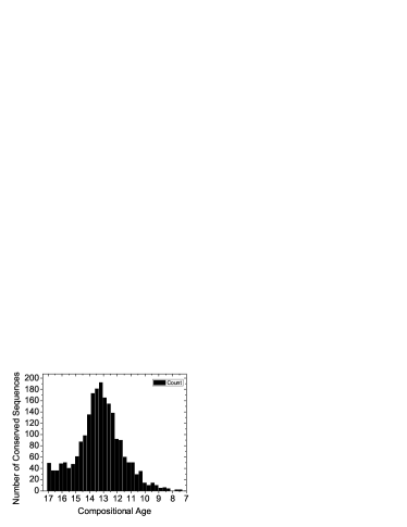
(a)

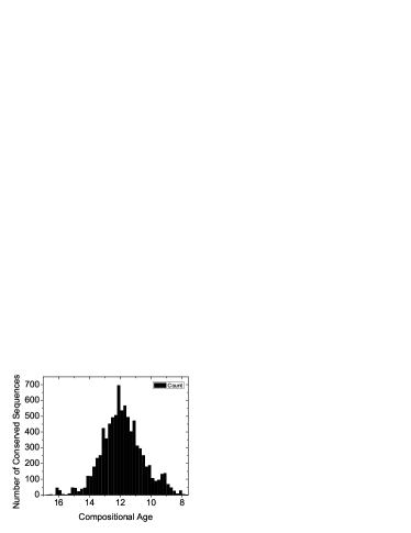
(b)

Figure 14: Distribution of conserved sequences with compositional age to find (a) age of LUCA, and (b) divergence time of fungi.

To find the divergence times of fungal proteins, we investigate 10 species of fungi. In the group Dikarya/Ascomycota/Saccharomycotina we choose S. cerevisiae, C. glabrata, K. lactis, Y. lipolytica, and P. stipitis. In the group Dikarya/Ascomycota/Pezizomycotina we choose N. crassa, M. grisea, and A. fumigatus. We find 8535 sequences with greater than 15 amino acids that appear in both branches and in at least 4 proteins. The histogram of compositional age of these sequences is shown in Fig. 14(b). The compositional age peaks at 12.1. We choose $1.1$ billion years ago as the real age of divergence time of these two branches of fungi Hedges (2002). So, the compositional age of 12.1 is corresponds to an age of 1.1 billion years ago.

To find the compositional age of recent proteins, we search for the youngest proteins in E. coli. We consider only proteins in the COG (Clusters of Orthologous Groups of proteins) database, to exclude those protein fragment without function in the FASTA file. We compare the proteins in two strains of E. coli: K12 and o157 :H7 EDL 933. The 0157 strain of E. coli diverged from K12 strain about 4 million years ago Reid et al. (2000). We take the strains of E. coli from the COG database that exclude the orthologous proteins that are shared by K12 and O157, which should be quite young, probably less than $4$ million years. The youngest new protein of O157 has compositional age of $9.607$. The youngest new protein of K12 has compositional age of $9.652$. We, therefore, set the compositional age of present day as $9.6$.

IV.2.2 Compositional Age and Evolutionary Rate

We want to find the relationship between the compositional age of proteins and the evolutionary rate of corresponding genes. The ratio of nonsynonymous substitution per site to synonymous substitution per site ($dN/dS$) is often assumed to be a good measure of evolutionary rate. Hirsh et al. compared the orthologous open reading frames in four yeast spices and provided $dN/dS$ data for 3392 genes Hirsh et al. (2005). Here we average the $dN/dS$ of proteins in every compositional age interval 0.2. For example, there are 326 proteins with compositional age between 10.9 and 11.1, we calculate the average $dN/dS$ 0.21 for those proteins and plot it in Fig. 15. The compositional age is negatively and nearly linearly related to the evolutionary rate (correlation coefficient $R^{2}=0.83$).

Figure 15: S. cerevisiae. The average $dN/dS$ is negatively linearly related to the compositional age.

IV.2.3 Growth of Modularity in the Protein-Protein Interaction Network

We quantify modularity of both protein domain structure and of the protein-protein interaction network Apic et al. (2001); Ng et al. (2003a, b). The protein-protein interaction network data come from DIP. We obtain 1846 proteins with 6971 interaction edges in E. coli and 3211 proteins with 17535 interaction edges in S. cerevisiae. The domain-domain interaction data come from InterDom. We consider only domain interactions based on the DIP database and take only these domain interactions with a score in the top 75%, to eliminate the noisy data. We obtain 276 proteins in E. coli and 427 proteins in S. cerevisiae, from which we extract the protein domains for study. Interestingly, the domain-domain interaction network is scale free with $\gamma=2.4$, see Fig. 16.

Figure 16: The degree distribution of the S. cerevisiae domain-domain interaction network.

To quantify modularity in the interaction networks, we construct the topological overlap matrix Ravasz et al. (2002) from the interaction network, reorder it with the average linkage clustering method Eisen et al. (1998), and normalize the number of interactions within modules according to network size. The topological overlap matrix element, $T_{ij}$, is the ratio of common nearest neighbors of the interacting proteins $i$ and $j$ to their respective degrees. The topological overlap matrix reflects the topological overlap of the nearest neighbors of two nodes. For any two nodes $i$ and $j$, the topological overlap is defined as Ravasz et al. (2002):

$$T_{ij}=\frac{\sum_{u}a_{iu}a_{uj}+a_{ij}}{\min(k_{i},k_{j})+1-a_{ij}}$$ (4)

Here $a_{ij}$ is the elements of the interaction network matrix with value 0 (not interacting) or 1 (interacting). We use the average-linkage hierarchical clustering algorithm Ravasz et al. (2002) to reorder the topological overlap matrix so that the more tightly linked and clustered nodes are moved close to each other. In this way, we identify the modules and hierarchical structure of the network.

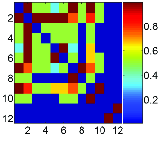
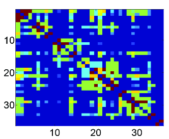
(a)                                                         (b)

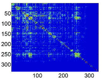
(c)                                                         (d)

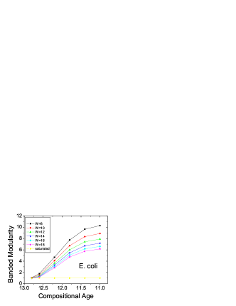
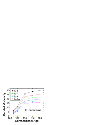
(e)                                                         (f)

Figure 17: (color online) The reordered topological overlap matrix of the E. coli protein interaction network constructed from proteins whose compositional age are larger than 12.8 (a), 12.6 (b), and 12.2 (c). The color reflects the strength of the topological overlap of two nodes (from 0.0 to 1.0), as shown in the color bar in (a). (d) The linear relationship between compositional age and real age. (e) and (f), The banded modularity evolution of E. coli and S. cerevisiae, respectively. The lines of different color in (e) and (f) correspond to different band sizes ($W$). Modularity grows with time. Banded modularity of a saturated matrix, i.e., a matrix with all elements being $1$ except the diagonal ones being $0$, is shown in (e) and (f) for comparison. The banded modularity of a saturated network is at its minimum value of $1$.

The reordered topological overlap matrix of E. coli at different times is shown in Fig. 17. The protein-protein interaction network evolves from an almost saturated, unstructured network in Fig. 17(a) to a mildly modular network with four modules in Fig. 17(b) and then to a highly modular network in Fig. 17(c). To compare the modularity quantitatively, we define banded modularity as the ratio of interaction within a diagonal band to the total interactions, normalized by the ratio of the area of the band to the area of the matrix:

$$M_{\rm banded}=\frac{\sum_{0<|i-j|<W}^{D}T_{ij}}{\sum_{i\neq j}^{D}T_{ij}}\times(\frac{\sum_{0<|i-j|<W}^{D}1}{\sum_{i\neq j}^{D}1})^{-1}$$ (5)

Here, $W$ is the width of the band, $D$ is the dimension of matrix and $T_{ij}$ is the element of reordered topological overlap matrix. Since the network size grows in time, we compare modularity of network of different sizes. The factor $1/({\sum_{0<|i-j|<W}^{D}1}/{\sum_{i\neq j}^{D}1})$ normalizes for the network size. In Fig. 17(e), we show the banded modularity grows with compositional age in E. coli. A similar result is observed for S. cerevisiae in Fig. 17(f). This result holds true for different band widths and different organisms; this phenomenon is robustly observed. In a modular structure, there are more interactions within a module than between modules. Banded modularity is a concise definition of modularity, but may also be interpreted as simply locality, in which true modules may not be identifiable.

To measure modularity in a more detailed way, we search along the diagonal of the reordered topological overlap matrix to find the explicit modules, and we calculate the ratio of interactions in the modules to the total interactions, normalized by the ratio of the area of modules to the area of the whole matrix. We define these modules quantitatively. First, we suppose the protein $i$ and $i+1$ form a module, and we ask whether another another protein $i+2$, should be added to the module. We add the protein if the average interaction between $i+2$ and the existing module is larger than a cutoff, which we set it 0.2 in our study. We continue this procedure. When we come to a protein with average interaction less than the cutoff, this protein forms the first member of a new module, and we begin the search to add further proteins to this new module. The modules so identified depend on the cutoff. In our study, the E. coli and S. cerevisiae networks are highly modular. We tried several cutoff and found the results are quite stable, with results in accord with our visual observation of the clustered matrix. We define the result as block modularity:

$$M_{\rm module}=\frac{\sum_{j,k\neq j=1}^{{}^{\prime}D}T_{jk}}{\sum_{j,k\neq j=1}^{D}T_{jk}}\times(\frac{\sum_{j,k\neq j=1}^{{}^{\prime}D}1}{D(D-1)})^{-1}$$ (6)

where in the upper sum with the prime, $k$ is over those proteins in the same module as $j$, $D$ is the dimension of the matrix.

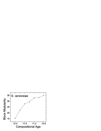
(a)                                                  (b)

Figure 18: Evolution of block modularity of protein interaction network in E. coli (a) and S. cerevisiae (b).

We apply this definition to the reordered topological overlap matrix to obtain the result for E. coli and S. cerevisiae in Fig. 18. We see the growth of block modularity in both organisms. There is a positive correlation between banded and block modularity. The growth of modularity is robust to the precise definition of modularity. The average size of module at different compositional age network is stable, see Fig. 19(a). The relationship between the size of the network and compositional age is show in Fig. 19(b). The average module size does not change much in evolution, and the number of proteins in each module in of S. cerevisiae is fewer than that in E. coli, perhaps reflecting that S. cerevisiae is more modular.

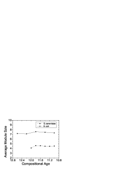
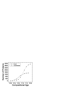
(a)                                                   (b)

Figure 19: (a) Average number of proteins in a module at different compositional ages, (b) Size of network in different compositional age network.

IV.2.4 Growth of Modularity in the Domain-Domain Interaction Network

We observed modularity not only in the protein-protein interaction network, but also in the domain-domain interaction network. We show the result of the banded modularity of the domain-domain interaction network of E. coli and S. cerevisiae in Fig. 20. The growth of banded modularity is pronounced in both cases.

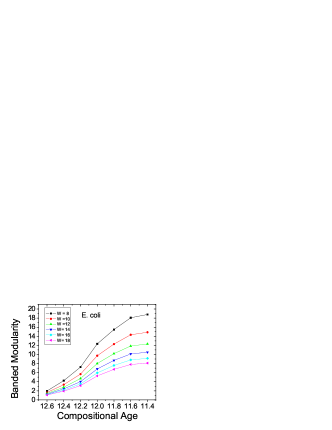
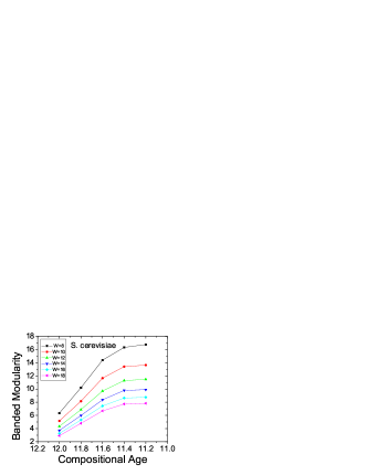
(a)                                                  (b)

Figure 20: (color online) Evolution of banded modularity of the domain-domain interaction network in E. coli (a) and S. cerevisiae (b).

Our definitions of modularity allows the comparison of modularity of matrices of different sizes. The saturated interaction matrix does not have any modular structure, regardless of the band size, as shown in Fig. 17(e),(f). A network generated by randomly selected proteins in E. coli is of constant low modularity (see Appendix B), independent of the number of proteins used. The network constructed based on its compositional age, however, shows a clear growth of its modularity. This result shows that the validity of organizing proteins by their compositional age.

We also measure modularity of the unweighted domain-domain interaction network directly, without construction of topological overlap matrix. We determine the fraction of a protein to which other proteins interact. To the extent that interactions become more localized within proteins, the protein is defined to be more modular. If protein B interacts with protein A, and the interaction is with only a few of the domains of protein A, then this interaction is more modular than if protein B interacts with a greater number of the domains of protein A. Averaging this measurement over all proteins B, this procedure gives us a measure of the modularity of protein A. So, we calculate the ratio of interacting domains to the number of domains in a protein, which gives the inverse of modularity. We define a Score, which is the inverse of modularity, as:

$$Score:\quad\frac{1}{2N}\sum_{l=1}^{N}\left(\frac{I^{A}_{l}}{D^{A}_{l}L^{2/3}_{B}}+\frac{I^{B}_{l}}{D^{B}_{l}L^{2/3}_{A}}\right)$$ (7)

Here $l$ represents a protein-protein interaction or a link. To distinguish the two proteins in a link, we mark one protein as A, the other one as B. The number of links is $N$. The term $L_{A}$ ($L_{B}$) is the number of amino acids of protein $A$ ($B$). The number of interacting domains is $I_{A}$, and the number of total domains is $D^{A}$ in protein $A$. We normalize the ratio of ${I^{A}}/{D_{A}}$ by the surface area of the target protein $L_{B}^{2/3}$, and so the Score should measure only the modularity and normalize out the size effect of target proteins.

(a)                                                  (b)

Figure 21: Domain interaction network modularity evolution in E. coli (a) and S. cerevisiae (b). Score is the inverse of modularity.

In Fig. 21, we compare the Scores of different domain-domain interaction network at different compositional age. The inverse of the Score increases monotonically with evolutionary progress. Because the inverse of the Score is modularity, we again observe that modularity has increased through time. This observation is robust under different definitions of the Score (see Appendix A).

IV.2.5 Summary

We have introduced several quantitative definitions of modularity for interacting networks. We use them to measure the modularity of the protein-protein interaction network and domain-domain interaction network in S. cerevisiae and E. coli. We have also introduced a method to quantify the evolutionary divergence time of proteins. We consistently find that modularity, by all definitions and in both organisms, appears to have grown through time. This observation is in agreement with the theory that environmental change coupled with horizontal gene transfer naturally and inevitably leads to evolution of increased modularity Sun and Deem (2007). In this sense, early life was a generalist, being less modular. As evolution proceeded, and diversity of species increased and the environment changed, proteins became more modular and specialized in their interactions.

V Conclusion

The model results were described at the individual level. In particular, we have presented the dynamics as that of individual short protein sequences in a population. The spin glass Hamiltonian, however, is a general description for the replication rate in evolution. The spin glass Hamiltonian captures two basic features of evolution: evolution is relatively slow, and there are many local fitness optima. Since the Hamiltonian captures the generic, basic features of evolution, we expect the emergence of modularity to be a generic, fundamental result.

Why is modularity so prevalent in the natural world? Our hypothesis is that a changing environment selects for adaptable frameworks, and competition among different evolutionary frameworks leads to selection of structures with the most efficient dynamics, which are the modular ones. We have provided experimental evidence supporting this hypothesis. We suggest that the beautiful, intricate, and interrelated structures observed in nature may be the generic result of evolution in a changing environment. The existence of such structure need not necessarily rest on intelligent design or the anthropic principle.

It is now believed that large scale exchange of genetic information is essential to increase the rate of evolution Shapiro (2002); Colegrave (2002); Goldenfeld and Woese (2007). Further experimental study of the relation between large scale genetic exchange and the promotion of modularity is warranted Misevic et al. (2006). Some species of yeast may undergo either sexual or asexual reproduction, and experiments suggest that yeasts undergoing sexual reproduction are more evolvable Goddard et al. (2005). It would be interesting to construct protocols to study the relation between sexual recombination and modularity, possibly in gene expression networks Soyer and Bonhoeffer (2006) in bacteria, in the laboratory. At an applied level, we note that the process by which antibiotics resistance evolved Walsh (2004) makes use of the modular structure of the genes encoding the enzymes that degrade and the pumps that excrete antibiotics and the modular structure of the proteins to which antibiotics bind Maiden (1998).

Appendix A Other Definitions of Domain Modularity

We consider several different definitions of a measure of modularity in protein domain interactions:

$$Score1:\quad \frac{1}{2N}\sum_{l=1}^{N}(\frac{I^{A}_{l}}{D^{A}_{l}}+\frac{I^{B}_{l}}{D^{B}_{l}})$$ (8)

$$Score2:\quad \frac{1}{N}\sum_{l=1}^{N}(\frac{P_{l}}{D^{A}_{l}D^{B}_{l}})$$ (9)

$$Score3:\quad \frac{1}{2N}\sum_{l=1}^{N}(\frac{I^{A}_{l}}{D^{A}_{l}L^{2/3}_{B}}+\frac{I^{B}_{l}}{D^{B}_{l}L^{2/3}_{A}})$$ (10)

$$Score4:\quad \frac{1}{2N}\sum_{l=1}^{N}(\frac{I^{A}_{l}}{D^{A}_{l}L^{B}}+\frac{I^{B}_{l}}{D^{B}_{l}L^{A}})$$ (11)

$$Score5:\quad \frac{1}{N}\sum_{l=1}^{N}(\frac{P_{l}}{D^{A}_{l}D^{B}_{l}L^{A}_{l}L^{B}_{l}})$$ (12)

$$Score6:\quad \frac{1}{N}\sum_{l=1}^{N}(\frac{P_{l}}{D^{A}_{l}D^{B}_{l}(L^{A}_{l})^{2/3}(L^{B}_{l})^{2/3}})$$ (13)

$$Score7:\quad \frac{1}{M}\sum_{l=1}^{N}(\sum_{j=1}^{D_{B}}\frac{T^{A}_{j}}{D^{A}_{l}}+\sum_{j=1}^{D_{A}}\frac{T^{B}_{j}}{D^{B}_{l}})$$ (14)

In Score1–Score6, $l$ represents a protein-protein interaction link. To distinguish the two proteins in each interaction link, we mark one protein as A, and the other one B. The number of protein-protein interaction links is $N$. The number of amino acids of protein $A$ ($B$) is $L^{A}$ ($L^{B}$). The number of total domains of protein $A$ is $D^{A}$. The number of domain-domain interaction links in the protein-protein interaction $l$ is $P_{l}$. Score1 measures the fraction of interacting domains to the total domains. Score2 measures the saturation of domain interactions. Score3 is refinement of Score1, excluding the effect of protein size by normalizing with the surface area of the substrate protein. Score4 is another alternative, in which the fraction of available contacts in the substrate is normalized simply by the number of amino acids. Score5 and Score6 are advanced versions of Score2, with normalizations for size of substrate. In Score7, we average over domain numbers instead of protein numbers. That is, when A interacts with B, B has $D_{B}$ domains; for the $j$th domain in protein B, it can interact with $T^{A}_{j}$ domains in protein A, and $M=\sum_{l=1}^{N}(D_{B}+D_{A})$. Score1–Score7 are all measures of the inverse of modularity. All of these scores show an increase of modularity through time, see Fig. 22.

Figure 22: Different definitions of inverse modularity, for E. coli and S. cerevisiae.

Appendix B Random Networks are Not Modular

We select 352 proteins in E. coli at random and find the interaction in DIP, then we construct the interaction network. The result after clustering, for E. coli at compositional age 12.2, is shown in Fig. 23. The E. coli network shows hierarchical structure, while the random network has no hierarchical structure. The selection by compositional age elucidates the non-random effects of evolution. We also use the random network to test the quality of our definition of block modularity. First, we calculate the degree of E. coli protein interaction network at different compositional ages, then, we construct several random networks with the same size and degree as the E. coli networks so constructed. We repeat this procedure 10 times for each point. We use the average linkage hierarchical clustering method to calculate the block modularity. We make a comparison with the E. coli network selected based on compositional age in Fig. 24. The E. coli networks are much more modular than are the random networks; the modularity of random networks is due only to random fluctuations that are grouped by the hierarchical clustering algorithm. The modules are visually apparent in the clustered matrix, as in Fig. 23(b).

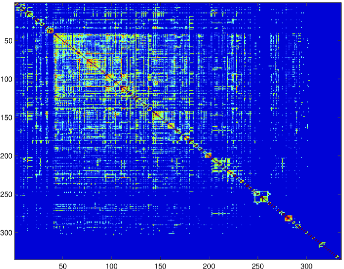
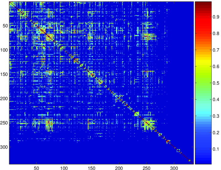
(a)                                                        (b)

Figure 23: (color online) (a) A random network. (b) E. coli protein interaction network at compositional age 12.2.

Figure 24: Comparison of banded modularity with width 8 between the E. coli network and the random network. The red line is the banded modularity of random network. The black line is the E. coli network with size 36 at compositional age 12.6, size 335 at compositional age 12.2, and size 949 at compositional age 11.8. Error bars are shown in blue.

References

- Shapiro (2004) J. A. Shapiro, Gene 345, 91 (2004).
- Shapiro (2005) J. A. Shapiro, BioEssays 27, 122 (2005).
- Misevic et al. (2006) D. Misevic, C. Ofria, and R. E. Lenski, Proc. R. Soc. B 273, 457 (2006).
- Shapiro (1992) J. A. Shapiro, Genetica 86, 99 (1992).
- Goldenfeld and Woese (2007) N. Goldenfeld and C. Woese, Nature 445, 369 (2007).
- Lipson et al. (2002) H. Lipson, J. B. Pollack, and N. P. Suh, Evolution 56, 1549 (2002).
- Tanase-Nicola et al. (2006) S. Tanase-Nicola, P. B. Warren, and P. R. tenWolde, Phys. Rev. Lett. 97, 068102 (2006).
- Variano et al. (2004) E. A. Variano, J. H. McCoy, and H. Lipson, Phys. Rev. Lett. 92, 188701 (2004).
- Shen-Orr et al. (2002) S. S. Shen-Orr, R. Milo, S. Mangan, and U. Alon, Nature Genetics 31, 64 (2002).
- Kashtan and Alon (2005) N. Kashtan and U. Alon, Proc. Natl. Acad. Sci. USA 102, 13773 (2005).
- Vetsigian et al. (2006) K. Vetsigian, C. Woese, and N. Goldenfeld, Proc. Natl. Acad. Sci. USA 103, 10696 (2006).
- Csete and Doyle (2002) M. E. Csete and J. C. Doyle, Science 295, 1664 (2002).
- Kitano (2004) H. Kitano, Nature Reviews Genetics 5, 826 (2004).
- Oikonomou and Cluzel (2006) P. Oikonomou and P. Cluzel, Nature Physics 2, 532 (2006).
- Earl and Deem (2004) D. J. Earl and M. W. Deem, Proc. Natl. Acad. Sci. USA 101, 11531 (2004).
- Deem (2007) M. W. Deem, Physics Today 60, 42 (2007).
- Gardener and Zuidema (2003) A. Gardener and W. Zuidema, Evolution 57, 1448 (2003).
- Sun and Deem (2007) J. Sun and M. W. Deem, Phys. Rev. Lett. 99, 228107 (2007).
- Kauffman and Levin (1987) S. Kauffman and S. Levin, J. Theor. Biol. 128, 11 (1987).
- Deem and Lee (2003) M. W. Deem and H.-Y. Lee, Phys. Rev. Lett. 91, 068101 (2003).
- Sun et al. (2005) J. Sun, D. J. Earl, and M. W. Deem, Phys. Rev. Lett. 95, 148104 (2005).
- Anderson (1983) P. W. Anderson, Proc. Natl. Acad. Sci. USA 80, 3386 (1983).
- Stein and Anderson (1984) D. L. Stein and P. W. Anderson, Proc. Natl. Acad. Sci. USA 81, 1751 (1984).
- Perelson and Macken (1995) A. S. Perelson and C. A. Macken, Proc. Natl. Acad. Sci. USA 92, 9657 (1995).
- Mezard et al. (1987) M. Mezard, G. Parisi, and M. Virasoro, Spin Glass Theory and Beyond: An Introduction to the Replica Method and Its Applications (World Scientific, New Jersey, 1987).
- Bogarad and Deem (1999) L. D. Bogarad and M. W. Deem, Proc. Natl. Acad. Sci. USA 96, 2591 (1999).
- Sun et al. (2006) J. Sun, D. J. Earl, and M. W. Deem, Mod. Phys. Lett. B 20, 63 (2006).
- Park and Deem (2007) J.-M. Park and M. W. Deem, Phys. Rev. Lett. 98, 058101 (2007).
- Barabási and Oltvai (2004) A. L. Barabási and Z. N. Oltvai, Nat. Rev. Genet. 5, 101 (2004).
- Gammaitoni et al. (1998) L. Gammaitoni, P. Hänggi, P. Jung, and F. Marchesoni, Rev. Mod. Phys. 70, 223 (1998).
- Sato et al. (2003) K. Sato, Y. Ito, T. Yomo, and K. Kaneko, Proc. Natl. Acad. Sci. USA 100, 14086 (2003).
- Parter et al. (2007) M. Parter, N. Kashtan, and U. Alon, BMC evolutionary biology 7, 169 (2007).
- Kreimer et al. (2008) A. Kreimer, E. Borenstein, U. Gophna, and E. Ruppin, Proc. Natl. Acad. Sci. U.S.A. 105, 6976 (2008).
- Singh et al. (2008) A. H. Singh, D. M. wolf, P. Wang, and A. P. Arkin, PNAS 105, 7500 (2008).
- Sobolevsky and Trifonov (2005) Y. Sobolevsky and E. N. Trifonov, J. Mol. Evol. 61, 591 (2005).
- Hedges (2002) S. B. Hedges, Nature 3, 838 (2002).
- Reid et al. (2000) S. D. Reid, C. J. Herbelin, A. C. Bumbaugh, R. K. Selander, and T. S. Whittam, Nature 406, 64 (2000).
- Hirsh et al. (2005) A. E. Hirsh, H. B. Fraser, and D. P. Wall, Molecular Biology and Evolution 22, 174 (2005).
- Apic et al. (2001) G. Apic, J. Gough, and S. A. Teichmann, J. Mol. Biol. 310, 311 (2001).
- Ng et al. (2003a) S. Ng, Z. Zhang, S. Tan, and K. Lin, Nucl. Acids Res. 31, 251 (2003a).
- Ng et al. (2003b) S. Ng, Z. Zhang, and S. Tan, Bioinformatics 19, 923 (2003b).
- Ravasz et al. (2002) E. Ravasz, A. L. Somera, D. A. Mongru, Z. N. Oltvai, and A. L. Barabási, Science 297, 1551 (2002).
- Eisen et al. (1998) M. B. Eisen, P. T. Spellman, P. O. Brown, and D. Botstein, Proc. Natl. Acad. Sci. USA 95, 14863 (1998).
- Shapiro (2002) J. A. Shapiro, J. Biol. Phys. 28, 745 (2002).
- Colegrave (2002) N. Colegrave, Nature 420, 664 (2002).
- Goddard et al. (2005) M. R. Goddard, H. C. J. Godfray, and A. Burt, Nature 434, 636 (2005).
- Soyer and Bonhoeffer (2006) O. S. Soyer and S. Bonhoeffer, Proc. Natl. Acad. Sci. USA 103, 16337 (2006).
- Walsh (2004) C. T. Walsh, Science 303, 1805 (2004).
- Maiden (1998) M. C. J. Maiden, Clin. Inf. Dis. 27S, S12 (1998).