SLAC-TN-09-002
B A B AR Note # 327
October 1996

Noise in a Calorimeter
Readout System
Using Periodic Sampling

Walter R. Innes
SLAC National Accelerator Laboratory

Fourier transform analysis of the calorimeter noise problem gives quantitative results on a) the time-height correlation, b) the effect of background on optimal shaping and on the ENC, c) sampling frequency requirements, and d) the relation between sampling frequency and the required quantization error.

1 Introduction

Noise in calorimeter readout electronics has been treated in some detail [Radeka, Haller, Dow]. However, since each author builds the details of their particular situation into their analysis, it is worthwhile to review the subject in light of our own experiment. Most previous studies assume that a single measurement will be made at a well determined time. Furthermore they assume that filtering preceding the digitization is limited to relatively simple analog devices. Since we have chosen to solve our lack of knowledge of the event time by recording periodic samples, applying digital signal processing techniques is natural. This also raises questions about the required sampling rate and the quantization error that don’t occur in the usual scheme.

Electronics noise and filters are usually analyzed using Fourier transforms [Ambrozny, Humphreys, Papoulis]. In the frequency domain, filtering, differentiation, integration, and time shifting are all represented by multiplications. Stochastic noise is most easily represented by its power spectral density (which is the Fourier transform of the more complicated auto-correlation function in the time domain). Many questions such as the signal to noise ratio for particular parameters and filter design can be handled entirely in the frequency domain.

2 The Input Circuit Model

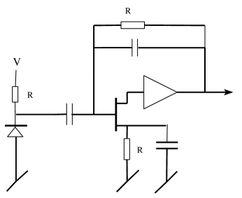
Figure 1: Simplified photodiode-preamp circuit

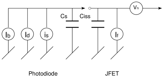
Figure 2: Model for the front end of the calorimeter readout. $i_{s}$ is the current due to the signal and is a function of time. $I_{d}$ is the spectral current noise generator corresponding to the shot noise of the photodiode. $I_{b}$ is the equivalent current noise caused by background photons from lost particles. $I_{f}$ is the FET input current noise, and $V_{n}$ is the FET input voltage noise. $C_{s}$ is the capacitance of the photodiode and $C_{iss}$ is the common source input capacitance of the FET.

Figure 1 shows a simplified version of the calorimeter input circuitry. Figure 2 shows a noise equivalent representation of the same circuit. The right hand portion represents the input FET. This is one of many possible equivalent representations [vanderZiel, page 29][Ambrozny, page 137]. This particular one has a relatively simple connection between the physical processes which generate noise and the elements of the representation. The spectral densities of the noise generators will correspond to the those given in manufacturers specification sheets.

2.1 The photo-diode

$i_{s}$ is a current generator corresponding to the signal generated by the interactions in the calorimeter. It will be represented by the function:

$$i_{s}(t)=\frac{1}{\tau_{s}}e^{-t/\tau_{s}}H(t).$$ (1)

$\tau_{s}$ is the decay time of the CsI(Tl) scintillation and $H(t)$ is the Heaviside unit step function. $\tau_{s}$ is 0.94$\,\mu\mbox{s}$ for CsI(Tl). The Fourier transform of $i(t)$ is

$$I_{s}(\omega)=\int_{-\infty}^{\infty}{i(t)e^{-j\omega t}\,dt}=\frac{1}{1+j\omega\tau_{s}}\ .$$ (2)

The spectral power density of the signal is:

$$I_{s}^{*}(\omega)I_{s}(\omega)=\frac{1}{1+\omega^{2}\tau_{s}^{2}}.$$ (3)

For characteristic times represented as $\tau_{x}$, I will use the notation that the associated radial velocity is $\omega_{x}\equiv 1/\tau_{x}$, the associated frequency is $f_{x}\equiv\omega_{x}/(2\pi)$, and the associated period is $T_{x}\equiv 1/f_{x}$. Using this notation we can write:

$$I_{s}(\omega)=\frac{-j\omega_{s}}{\omega-j\omega_{s}}\ \ {\rm and}\ \ I_{s}^{*}(\omega)I_{s}(\omega)=\frac{\omega_{s}^{2}}{\omega^{2}+\omega_{s}^{2}}.$$ (4)

$I_{d}$ is the current generator corresponding to the shot noise caused by the leakage current in the photodiode. This has a “white” (independent of $\omega$) spectrum with the value $I_{d}^{2}=2eI_{leak}$ (units of current squared per bandwidth). The order of magnitude for $I_{leak}$ is nanoamperes. We’ll assume our diode has a leakage of 4 nA. Since we average two diodes we can use the equivalent leakage of 2 nA for a single diode giving $I_{d}=25\mbox{\,fA}/\rm\sqrt{\mbox{\,Hz}}$.

$C_{s}$ is the capacitance of the back-biased photodiode. A typical value is 80 pF, which we’ll use in our estimates.

A photodiode with these properties is the 1N2744.

As much as possible, the discussion will be restricted to the electronic regime. However, some effects depend on the efficiency of the conversion of calorimeter shower energy into charge. When this number is required, I will use the value of 3000 photo-electrons per MeV in each diode.

2.2 The FET

$C_{iss}$ is the FET common source input capacitance. It can range from a few picofarads to tens of picofarads depending on the choice of FET. We will return to this choice later. In the circuit it functions in parallel with $C_{s}$. Not shown in the figure since they are much less than $C_{s}$ are the feedback capacitance $C_{f}$ and the calibration injection capacitance $C_{cal}$. I will call the sum $C_{s}+C_{iss}+C_{f}+C_{cal}$ simply $C$.

$I_{f}$ is a noise generator corresponding the input current noise of the FET. It is primarily due to the gate leakage current, although for very large gate areas the effect the thermal noise of the real part of the input impedance should be checked. The shot noise acts just like the diode shot noise and the two leakage currents may be added. In practice the FET gate leakage current is of the order of picoamperes and is negligible compared to the diode leakage current. Let $I_{n}^{2}=I_{d}^{2}+I_{f}^{2}\approx I_{d}^{2}$.

$V_{n}$ is a voltage noise generator representing the input voltage noise of the FET. This is primarily due the thermal noise in the FET channel. Many authors put a formula, which shows the dependence of this noise on the temperature and the forward transconductance, into their equations [vanderZiel, page 75]. I prefer to keep $V_{n}$ as an explicit term. The value of $V_{n}$ is usually given on specification sheets and is also easy to measure. For junction FETs, $V_{n}$ is approximately independent of frequency over the range of interest to us. Typical values are 1 to 2 nV/$\rm\sqrt{\mbox{\,Hz}}$.

In order to be more specific I’ll take as an example the SANYO 2SK932 JFET. $C_{iss}$ is 20 pF and $V_{n}$ is $\approx 0.7\mbox{\,nV}/\rm\sqrt{\mbox{\,Hz}}$. Because we average the outputs two diode-FET-preamp combinations on each crystal, we divide by $\sqrt{2}$ to get 0.5 nV/$\rm\sqrt{\mbox{\,Hz}}$. This is a good FET but not optimally matched to our problem. We’ll return to this issue after we have developed the signal to noise formulas.

Figure 3: The amplitude spectra of the various noise sources expressed as input current densities. For the background, nominal conditions are assumed and no energy cutoff is used. Note that the signal has the same spectrum as the background noise.

2.3 Background

$I_{b}$ is a current noise generator representing the sea of photons generated by particles lost from the beam. This noise resembles shot noise in that near impulsive elements arrive at random times. It differs in that the pulse shape is not a delta function but has the shape of the signal and there is a distribution of pulse areas instead of just the electron charge. If we return to the derivation of the shot noise formula [Ambrozny, page 81], we see that the first difference can be treated by giving this noise the power spectrum of the signal (the Fourier transform of each pulse is the same as that of the signal except for phase and magnitude). The second is handled by noting that the shot noise formula is really a pulse area squared times a rate: $I_{d}^{2}=2e^{2}f_{leak}$. $e$ is the size of the pulse and $f_{leak}$ is the mean rate of their occurrence. Therefore we can get the low frequency limit of the noise spectral density of the background by doing the integral:

$$I_{b}^{2}=\int_{0}^{\infty}{2q^{2}B(q)\,dq}$$ (5)

where $B$ is the rate of background events per pulse area interval per time interval. The value of this integral can be inferred from the statistics of histograms such as those in B A B AR Technical Design Report Figure 12-9 [BaBar]. Here I use more recent calculations of the background [Marsiske]. Assuming $3000\rm\,pe/\mbox{\,Me\kern-0.80002ptV}/diode$, the result for an average crystal is $I_{b}=460\mbox{\,fA}/\rm\sqrt{\mbox{\,Hz}}$ at nominal background.

For convenience I’ll use the symbol $I_{b}$ to represent this low frequency limit and put the frequency dependence into the formulas explicitly. Since $I_{n}$ and $V_{n}$ are approximately independent of frequency, I can then treat $I_{b}$, $I_{n}$, and $V_{n}$ as constants.

Note that individual crystals can differ from the average by factors as large as $4$. In particular, compared an average barrel crystal, an average endcap crystal has $5/7$th the hit rate, twice the average energy deposit, and an $I_{b}$ twice as large.

Figure 3 summarizes all the noise sources.

2.3.1 Limitations

The treatment of background as noise is a good description if the background signal after all processing contains significant contributions from many background events. If this is not the case, the data may fall into two classes, those showers little affected by background, and those with a large background contribution. The former will have a distribution of measured values consistent with electronic noise, while the latter may have a wider, highly skewed distribution. While the background as noise treatment may give a near optimal procedure for minimizing the rms error, it will widen the distribution for that class events unaffected by background. Depending on the physics objective, treating the background affected events as an inefficiency rather than events with errors may give the better result.

How well does our case satisfy this many hit condition? In the background calculation in the preceding paragraph, an average crystal had $0.11\,\rm hits/crystal/\,\mu\mbox{s}$. Assuming a window of $2\,\mu\mbox{s}$ and a sum of 25 crystals, this implies 5.5 background hits contributing to the measurement during nominal conditions. This is enough to give reasonably Guassian behavior. However, much of $I_{b}$ is generated by the high energy tail of the background distribution. If we count down from high energies until get a mean number of hits of at least 2, the cut would be in the vicinity of $1\mbox{\,Me\kern-0.80002ptV}$. At 10 times nominal this cut would be close to $3\mbox{\,Me\kern-0.80002ptV}$.

Another consideration is that an approach which tries to separate a background tail from other noise is hardly likely to succeed if the magnitude of the background contribution is of the same size as other errors. The size of the intrinsic error depends on the size of the signal. For a $100\mbox{\,Me\kern-0.80002ptV}$ shower the expected error is $\approx 2\mbox{\,Me\kern-0.80002ptV}$. Assuming that background contributions must be at least $3\mbox{\,Me\kern-0.80002ptV}$ before they can be separated from noise seems conservative.

If only background hits with energies below $3\mbox{\,Me\kern-0.80002ptV}$ are included, $I_{b}$ falls to $160\mbox{\,fA}/\rm\sqrt{\mbox{\,Hz}}$. The background rate falls to $0.10\,\rm hits/crystal/\,\mu\mbox{s}$.

3 Theorems

3.1 $S/N$

The Radar Handbook [Skolnik, page 4-11] reviews the theory of finding a known signal in noise from the starting point of doing a least square fit to a finite set of measurements. Under fairly general conditions this is equivalent to the maximum likelihood fit and is the best that can be done. The treatment proceeds by taking the continuous infinite time limit which turns the usual matrix equations into integral equations. These are then solved by applying Fourier transforms. For a signal $i(t,a_{1},...,a_{n})$ with Fourier transform $I(\omega,a_{1},...,a_{n})$ the elements of the inverse of the error matrix for $a_{i}$ are given by:

$$[{\bf V}^{-1}]_{ik}=\frac{1}{2\pi}\int_{-\infty}^{\infty}{\left(\left(\frac{\partial I(\omega)}{\partial a_{i}}\frac{\partial I^{*}(\omega)}{\partial a_{k}}\right)/N(\omega)\right)d\omega},$$ (6)

where $N$ is the double sided noise power spectral density. This matrix is known as the information matrix and also as the signal to noise ratio ($S/N$) matrix.

In our case the signal has two parameters, amplitude and time offset:

$$i(t)=ai_{0}(t-t_{0}).$$ (7)

This has the Fourier transform

$$I(\omega)=aI_{0}(\omega)e^{-j\omega t_{0}}.$$ (8)

If we define $I_{0}$ such that the actual value of $a$ is 1 we find

$$\frac{\partial I}{\partial a} = I(\omega)\mbox{,\rm\hskip 72.26999pt and}$$ (9)

$$\frac{\partial I}{\partial t_{0}} = -j\omega I(\omega).$$ (10)

Thus the matrix of integrands in the $S/N$ formula is

$$\left[\begin{array}[]{cc}~{}~{}~{}1{}{}{}&~{}~{}j\omega{}{}\\ -j\omega&\omega^{2}\end{array}\right]\frac{|I(\omega)|^{2}}{N(\omega)}$$ (11)

Because both $|I(\omega)|^{2}$ and $N(\omega)$ are even in $\omega$, the integral of the off-diagonal elements is 0. Since the matrix is diagonal, inverting it to get the error matrix ${\bf V}$ is trivial. If $i(t)$ is normalized to unit area, the $aa$ element of ${\bf V}$ is the square of the equivalent noise charge (ENC) and the $t_{0}t_{0}$ element is the square of product of the pulse height and the time error (ENTC). Since there is no correlation between these errors, a priori knowledge of the time does not improve the determination of the amplitude. The final formulas for the signal to noise are:

$$\left[\frac{S}{N}\right]_{aa}=\frac{1}{2\pi}\int_{-\infty}^{\infty}{\frac{|I(\omega)|^{2}}{N(\omega)}\,d\omega},\\$$ (12)

and

$$\left[\frac{S}{N}\right]_{tt}=\frac{1}{2\pi}\int_{-\infty}^{\infty}{\frac{|I(\omega)|^{2}}{N(\omega)}\,\omega^{2}d\omega}$$ (13)

3.2 Matched filter

This result for the error in the amplitude is the same that is given in many texts as the best that can be achieved using an optimal matched filter [Humphreys, page 65][Papoulis, page 135]. Assume there exists a filter such that the output peaks at $t=0$. The square of that peak value is given by:

$$o^{2}(0)=\left|\frac{1}{2\pi}\int_{-\infty}^{\infty}{I(\omega)F(\omega)\,d\omega}\right|^{2},$$ (14)

where $F(\omega)$ is the transfer function of the filter. The mean square noise after filtering is the same at all times and is given by

$$n_{o}^{2}=\frac{1}{2\pi}\int_{-\infty}^{\infty}{N(\omega)|F(\omega)|^{2}\,d\omega}.$$ (15)

The signal to noise is the ratio of $o^{2}(0)$ to $n_{o}^{2}$. Multiplying the integrand of the numerator by $\sqrt{N(\omega)}/\sqrt{N(\omega)}$ and using Schwarz’s inequality proves that the signal to noise is less than or equal to the $S/N$ derived from the least square fit method (equation 12). Furthermore, inspection of the $S/N$ equation before this manipulation shows that the equality can be achieved using a filter with a transfer function of

$$F(\omega)\propto\frac{I^{*}(\omega)}{N(\omega)}\ .$$ (16)

From this I conclude that the best possible result can be achieved with a filter technique and that the required filter is readily calculated given knowledge of the shape of the signal and the spectrum of the noise.

The impulse response to the optimal filter is

$$f(t)\propto\frac{1}{2\pi}\int_{-\infty}^{\infty}{\frac{I^{*}(\omega)}{N(\omega)}\,e^{j\omega t}d\omega}\ ,$$ (17)

and the shape of a noiseless signal after filtering (the convolution of the signal with impulse response) is

$$o(t)\propto\frac{1}{2\pi}\int_{-\infty}^{\infty}{\frac{|I(\omega)|^{2}}{N(\omega)}\,e^{j\omega t}d\omega}\ .$$ (18)

A useful normalization for the filter can be achieved by dividing by the signal to noise ratio (equation 12). This yields $o(0)=1$. In the following discussion, $F$, $f$, and $o$ are so normalized.

4 Application to our problem

We have now collected all the necessary input information and the tools we need to design an optimal filter and calculate the signal to noise. Before tackling the full problem lets explore some special cases so that we can get an understanding of the effect of each input, can compare our results with previous work, and gain confidence in the method. Some of the formulas are followed by a bracketed reference to the source of the evaluation of the previous integral. Actually most of the integrals are straightforward (but sometimes tedious) to do using contour integration. This is a consequence of the fact that the signals, backgrounds, and analog filters all have exponential shapes in the time domain. More general signal shapes are less tractable.

4.1 No background ($I_{b}=0$) and $\tau_{s}=0$

This is the usual treatment when the “ballistic deficit” is ignored. $i_{s}(t)$ is a delta function, $I_{s}(\omega)=1$, and $2N(\omega)=I_{n}^{2}+V_{n}^{2}\omega^{2}C^{2}$.

Before starting lets evaluate some useful constants related to the inputs so that we can use them to evaluate the results as we go: $\tau_{n}\equiv V_{n}C/I_{n}=2.0\,\mu\mbox{s}$, $\omega_{n}\equiv 1/\tau_{n}=0.50\rm\,M\,radians/s$, and $f_{n}=80\mbox{\,kHz}$.

$$\left[\frac{S}{N}\right]_{aa} = \frac{\omega_{n}^{2}}{\pi I_{n}^{2}}\int_{-\infty}^{\infty}{\frac{1}{\omega_{n}^{2}+\omega^{2}}\,d\omega}$$ (19)

$$= \frac{\omega_{n}}{I_{n}^{2}}$$ (20)

$$ENC^{2} = I_{n}^{2}\tau_{n}=I_{n}V_{n}C$$ (21)

$$\left[\frac{S}{N}\right]_{tt} = \frac{\omega_{n}^{2}}{\pi I_{n}^{2}}\int_{-\infty}^{\infty}{\frac{\omega^{2}}{\omega_{n}^{2}+\omega^{2}}\,d\omega}$$ (22)

$$= \infty$$ (23)

$$ENTC^{2} = 0$$ (24)

$$F(\omega) = \frac{2\omega_{n}}{\omega_{n}^{2}+\omega^{2}}$$ (25)

$$f(t) = e^{-|t|/\tau_{n}}$$ (26)

$$o(t) = e^{-|t|/\tau_{n}}$$ (27)

Substituting our sample values, we find that $ENC=223\,e$, and the corner frequency of the optimal filter is 80 kHz.

4.2 No background ($I_{b}=0$) and $\tau_{s}>0$

This is the case usually treated, ballistic deficit included.

$$I_{s}(\omega) = \frac{-j\omega_{s}}{\omega-j\omega_{s}}$$ (28)

$$2N(\omega) = (I_{n}^{2}+V_{n}^{2}\omega^{2}C^{2})=I_{n}^{2}(\omega^{2}+\omega_{n}^{2})/\omega_{n}^{2}$$ (29)

$$\left[\frac{S}{N}\right]_{aa} = \frac{\omega_{s}^{2}\omega_{n}^{2}}{\pi I_{n}^{2}}\int_{-\infty}^{\infty}{\frac{1}{(\omega^{2}+\omega_{s}^{2})(\omega^{2}+\omega_{n}^{2})}\,d\omega}$$ (30)

$$= \frac{\omega_{s}\omega_{n}}{I_{n}^{2}(\omega_{s}+\omega_{n})}\mbox{\hskip 72.26999pt \rm[Dwight~{}856.31]}$$ (31)

$$ENC^{2} = I_{n}^{2}(\tau_{n}+\tau_{s})=I_{n}V_{n}C+I_{n}^{2}\tau_{s}$$ (32)

$$\left[\frac{S}{N}\right]_{tt} = \frac{\omega_{s}^{2}\omega_{n}^{2}}{\pi I_{n}^{2}}\int_{-\infty}^{\infty}{\frac{\omega^{2}}{(\omega^{2}+\omega_{s}^{2})(\omega^{2}+\omega_{n}^{2})}\,d\omega}$$ (33)

$$ENTC^{2} = I_{n}^{2}\tau_{n}\tau_{s}(\tau_{n}+\tau_{s})=ENC^{2}\tau_{n}\tau_{s}\mbox{\hskip 36.135pt \rm[Maple]}$$ (34)

$$F(\omega) = \frac{2j\omega_{n}(\omega_{n}+\omega_{s})}{(\omega+j\omega_{s})(\omega^{2}+\omega_{n}^{2})}$$ (35)

$$f(t) = \frac{\omega_{n}(\omega_{n}+\omega_{s})}{\pi}\int_{-\infty}^{\infty}{\frac{(\omega_{s}+j\omega)}{(\omega^{2}+\omega_{s}^{2})(\omega^{2}+\omega_{n}^{2})}e^{j\omega t}d\omega}$$ (36)

$$= \frac{\omega_{n}(\omega_{n}+\omega_{s})}{(\omega_{n}^{2}-\omega_{s}^{2})}\left(e^{-|t|/\tau_{s}}-\frac{\omega_{s}}{\omega_{n}}e^{-|t|/\tau_{n}}-\rm signum(t)\left(e^{-|t|/\tau_{s}}-e^{-|t|/\tau_{n}}\right)\right)$$ (37)

$$= \left(e^{-|t|/\tau_{n}}+H(-t)\frac{2\tau_{s}}{\tau_{n}-\tau_{s}}\left(e^{-|t|/\tau_{n}}-e^{-|t|/\tau_{s}}\right)\right)$$ (38)

$$o(t) = \frac{\omega_{n}\omega_{s}(\omega_{n}+\omega_{s})}{\pi}\int_{-\infty}^{\infty}{\frac{e^{j\omega t}}{(\omega^{2}+\omega_{s}^{2})(\omega^{2}+\omega_{n}^{2})}\,d\omega}$$ (39)

$$= \frac{1}{(\tau_{n}-\tau_{s})}\left(\tau_{n}e^{-|t|/\tau_{n}}-\tau_{s}e^{-|t|/\tau_{s}}\right)$$ (40)

Substituting our sample values, we find that $ENC=239\,e$, $ENTC=327\,\mu\mbox{s}\,e$ (1.1 ns for a 100 MeV deposit), and the corner frequency of the optimal filter is still 80 kHz. The ENC corresponds to and equivalent noise energy (ENE) of 80 keV.

4.3 $I_{b}>0$, $V_{n}=0$, and $I_{n}=0$

This special case of no electronic noise is explored to give us confidence that the filter technique does separate the desired signal from the background noise.

$$I_{s}(\omega) = \frac{-j\omega_{s}}{\omega-j\omega_{s}}$$ (41)

$$2N(\omega) = \frac{\omega_{s}^{2}I_{b}^{2}}{\omega_{s}^{2}+\omega^{2}}$$ (42)

$$\frac{|I_{s}|^{2}}{N} = \frac{2}{I_{b}^{2}}$$ (43)

$$\left[\frac{S}{N}\right]_{aa} = \infty\ ,\ ENC^{2}=0$$ (44)

$$\left[\frac{S}{N}\right]_{tt} = \infty\ ,\ ENCT^{2}=0$$ (45)

$$f(t) \propto \frac{1}{\pi}\int_{-\infty}^{\infty}{(\omega_{s}-j\omega)e^{j\omega t}d\omega}$$ (46)

$$\propto 2\left(\delta(t)-\tau_{s}\delta^{\prime}(t)\right)$$ (47)

$$o(t) \propto \frac{1}{\pi}\int_{-\infty}^{\infty}{e^{j\omega t}d\omega}\,\,\propto\,\,2\delta(t)$$ (48)

Because the signal and (background) noise have the same spectrum, the signal to noise ratio is independent of frequency. This results in infinite signal to noise integrals and no error on the pulse height and time determinations. In the absence of other noise, the matched filter turns both the signal and background events into delta functions which are always separable.

4.4 The general case

Now we will treat our general case, with all noise and width processes active. The signal is as for the previous two cases. The noise is the sum of the noise in those cases.

$$I_{s}(\omega) = \frac{-j\omega_{s}}{\omega-j\omega_{s}}$$ (49)

$$|I_{s}(\omega)|^{2} = \frac{\omega_{s}^{2}}{\omega_{s}^{2}+\omega^{2}}$$ (50)

$$2N(\omega) = \frac{I_{n}^{2}}{\omega_{n}^{2}}(\omega_{n}^{2}+\omega^{2})+\frac{\omega_{s}^{2}I_{b}^{2}}{\omega_{s}^{2}+\omega^{2}}$$ (51)

$$\left[\frac{S}{N}\right]_{aa} = \frac{\omega_{s}^{2}\omega_{n}^{2}}{\pi I_{n}^{2}}\int_{-\infty}^{\infty}{\frac{1}{\omega^{4}+(\omega_{s}^{2}+\omega_{n}^{2})\omega^{2}+\omega_{n}^{2}\omega_{s}^{2}(1+I_{b}^{2}/I_{n}^{2})}\,d\omega}$$ (52)

$$b^{2} \equiv 1+I_{b}^{2}/I_{n}^{2}\mbox{\hskip 36.135pt\rm and\hskip 36.135pt }\omega_{b}\equiv\omega_{n}b$$ (53)

$$\left[\frac{S}{N}\right]_{aa} = \frac{\omega_{s}\omega_{b}}{(I_{n}^{2}+I_{b}^{2})\sqrt{2\omega_{b}\omega_{s}+(\omega_{n}^{2}+\omega_{s}^{2})}}\mbox{\hskip 72.26999pt \rm[Dwight~{}857.11]}$$ (54)

$$ENC^{2} = (I_{n}^{2}+I_{b}^{2})\sqrt{\tau_{b}\tau_{s}}\sqrt{2+\tau_{b}/\tau_{s}+\tau_{s}/(b^{2}\tau_{b})}$$ (55)

$$\left[\frac{S}{N}\right]_{tt} = \frac{\omega_{s}^{2}\omega_{n}^{2}}{\pi I_{n}^{2}}\int_{-\infty}^{\infty}{\frac{\omega^{2}}{\omega^{4}+(\omega_{s}^{2}+\omega_{n}^{2})\omega^{2}+\omega_{n}^{2}\omega_{s}^{2}(1+I_{b}^{2}/I_{n}^{2})}\,d\omega}$$ (56)

$$ENTC^{2} = I_{n}^{2}\tau_{n}\tau_{s}\sqrt{\tau_{n}^{2}+\tau_{s}^{2}+2b\tau_{n}\tau_{s})}=ENC^{2}\tau_{b}\tau_{s}\mbox{\hskip 25.29494pt\rm[Prudnikov 2.2.10 \#4 page 313]}\hfil$$ (57)

$$F(\omega) = ENC^{2}\,\,\frac{2\omega_{s}\omega_{n}^{2}(\omega_{s}+j\omega)}{I_{n}^{2}(\omega^{4}+(\omega_{s}^{2}+\omega_{n}^{2})\omega^{2}+\omega_{s}^{2}\omega_{n}^{2}b^{2})}$$ (58)

$$f(t) = ENC^{2}\,\,\frac{\omega_{s}\omega_{n}^{2}}{\pi I_{n}^{2}}\int_{-\infty}^{\infty}{\frac{(\omega_{s}+j\omega)e^{j\omega t}}{(\omega^{4}+(\omega_{s}^{2}+\omega_{n}^{2})\omega^{2}+\omega_{s}^{2}\omega_{n}^{2}b^{2})}d\omega}$$ (59)

$$= ENC^{2}\,\,\frac{2\omega_{s}\omega_{n}^{2}}{\pi I_{n}^{2}}\left(\int_{0}^{\infty}{\frac{\omega_{s}\cos(\omega t)-\omega\sin(\omega t)}{(\omega^{4}+(\omega_{s}^{2}+\omega_{n}^{2})\omega^{2}+\omega_{s}^{2}\omega_{n}^{2}b^{2})}d\omega}\right)$$ (60)

$$\omega_{+} \equiv \sqrt{(\omega_{b}\omega_{s}+(\omega_{s}^{2}+\omega_{n}^{2})/2)/2}$$ (61)

$$\omega_{-} \equiv \sqrt{(\omega_{b}\omega_{s}-(\omega_{s}^{2}+\omega_{n}^{2})/2)/2}$$ (62)

$$f(t) = ENC^{2}\,\,\frac{\omega_{n}\omega_{s}}{2I_{n}^{2}}e^{-\omega_{+}|t|}\left(\frac{1}{b\omega_{+}}\cos(\omega_{-}t)+\frac{1}{b\omega_{-}}\sin(\omega_{-}|t|)-\frac{\omega_{n}}{\omega_{+}\omega_{-}}\sin(\omega_{-}t)\right)$$

                                                       [Prudnikov 2.5.10 #15 and#17 page 397]

$$= e^{-|t|/\tau_{+}}\left(\cos(t/\tau_{-})+\left(\frac{\tau_{-}}{\tau_{+}}\rm signum(t)-\frac{\tau_{+}}{\tau_{b}}\right)\sin(t/\tau_{-})\right)$$ (64)

$$o(t) = ENC^{2}\,\frac{\omega_{n}^{2}\omega_{s}^{2}}{\pi I_{n}^{2}}\int_{-\infty}^{\infty}{\frac{e^{j\omega t}}{(\omega^{4}+(\omega_{s}^{2}+\omega_{n}^{2})\omega^{2}+\omega_{s}^{2}\omega_{n}^{2}b^{2})}\,d\omega}$$ (65)

$$= e^{-|t|/\tau_{+}}\left(\cos(t/\tau_{-})+\frac{\tau_{-}}{\tau_{+}}\sin(|t|/\tau_{-})\right)$$ (66)

The filter output for a noiseless signal pulse is shown in Figure 4.

Figure 4: A noiseless signal after passing through the optimal filter. The peak gives the estimate for the signal charge and time. In this case t=0 and the charge is unity.

4.5 $I_{n}=0$, $\omega_{s}<<\omega_{b}$

The results in the previous section are a bit complex, but can be simplified for our case if we note that $I_{b}$ is more than 10 times $I_{n}$ even at nominal background levels. In addition, $\omega_{b}$ is more than five times $\omega_{s}$. Setting $I_{n}=0$, using the approximation $\omega_{b}>>\omega_{s}$, and defining $\omega_{sb}\equiv\sqrt{\omega_{b}\omega_{s}/2}\approx\omega_{-}\approx\omega_{+}$, we find:

$$I_{s}(\omega) = \frac{-j\omega_{s}}{\omega-j\omega_{s}}$$ (67)

$$|I_{s}(\omega)|^{2} = \frac{\omega_{s}^{2}}{\omega^{2}+\omega_{s}^{2}}$$ (68)

$$2N(\omega) \approx \frac{I_{b}^{2}(\omega^{4}+4\omega_{sb}^{4})}{\omega_{b}^{2}(\omega^{2}+\omega_{s}^{2})}$$ (69)

$$|I_{s}(\omega)|^{2}/N(\omega) \approx \frac{8\omega_{sb}^{4}}{I_{b}^{2}(\omega^{4}+4\omega_{sb}^{4})}$$ (70)

$$ENC^{2} \approx I_{b}^{2}\tau_{sb}=\sqrt{2\tau_{s}I_{b}^{3}V_{n}C}$$ (71)

$$ENTC^{2} \approx ENC^{2}\tau_{s}\tau_{b}=\sqrt{2I_{b}\tau_{s}^{3}V_{n}^{3}C^{3}}$$ (72)

$$F(\omega) \approx \frac{j\omega_{b}\omega_{sb}(\omega-j\omega_{s})}{(\omega^{4}+4\omega_{sb}^{4})}$$ (73)

$$f(t) \approx e^{-|t|/\tau_{sb}}\left(\cos(t/\tau_{sb})+\sin(|t|/\tau_{sb})-\sqrt{2\tau_{s}/\tau_{b}}\sin(t/\tau_{sb})\right)$$ (74)

$$o(t) \approx e^{-|t|/\tau_{sb}}\left(\cos(t/\tau_{sb})+\sin(|t|/\tau_{sb})\right)$$ (75)

Figure 5: The optimal filter in the frequency domain.

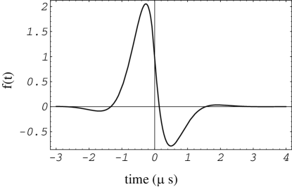
Figure 6: The optimal filter in the time domain.

The optimal filter is shown in the frequency and time domains in Figures 5 and 6.

Now for some values: $\tau_{b}=V_{n}C/I_{b}=0.11\,\mu\mbox{s}$, the filter corner $\sqrt{\tau_{s}\tau_{b}}=0.32\,\mu\mbox{s}$, $ENC=1930$ e, and $ENTC=620$$\,\mu\mbox{s}$ e or 2.1 ns for a 100 MeV deposit. The frequency corner of the optimum filter is 0.50 MHz.

For our worst case of times $10\times$nominal background, $I_{b}$ goes up $\times 3.1$, $\tau_{b}$ goes down $\times 3.1$, and $\sqrt{\tau_{s}\tau_{b}}$ goes down $\times 1.78$ to 0.17$\,\mu\mbox{s}$. $ENC=4460\,e$, $ENTC=760\,\mu\mbox{s}\,e$, and the corner frequency goes to $0.90\mbox{\,MHz}$. If the $3\mbox{\,Me\kern-0.80002ptV}$ cut were used to calculate $I_{b}$, $I_{b}$ would be lower by a factor of $2.4$ and the values for $\times 10$ would be about the same as the uncut nominal values.

5 Picking the best FET

We see that the $ENC$ depends on the FET properties only in the combination $V_{n}$($C_{iss}$+$C_{s}$). The smaller this value the better. For a given FET design, these parameters can be varied by changing the gate area $A$ (or equivalently connecting FETs in parallel). $V_{n}$ decreases as $1/\sqrt{A}$ while $C_{iss}$ is proportional to $A$. $V_{n}$$C$ is a minimum with respect to $A$ when $C_{iss}=C_{s}$. This implies that our sample FET should be scaled to 4 times its original gate area. Making this change would decrease $V_{n}$$C$ by a factor of 1.25. Since $ENC$ goes as the fourth root of $V_{n}$$C$, $ENC$ would decrease only 5%. On the other hand, $ENTC$ would decrease by 16%.

6 Sampling Requirements

So far we have assumed that the signals are ideally and continuously measured. In fact they will be sampled with limited precision. What restrictions on the sampling rate, length, and accuracy will prevent the loss of information?

6.1 Sampling frequency

The sampling frequency must be high enough to capture all frequencies with useful $S/N$. It must also be high enough to avoid misrepresenting noise at higher frequencies as noise in the signal region (aliasing). On the other hand the sampling frequency should be no higher than necessary.

What is the highest useful frequency? We note that $S/N$ is approximately constant up to $\omega=\omega_{sb}$ and then decreases as $1/\omega^{4}$. If we throw away all information above $\omega=\omega_{c}$ the fraction of information lost is approximately $(3/4)(\omega_{sb}/\omega_{c})^{3}$. For a 20% loss of information this implies that $\omega_{c}\geq 1.5\omega_{sb}$, and that $f_{c}>0.6\mbox{\,MHz}$. The fractional loss in time signal noise is somewhat larger, being given approximately by $(3/4)(\omega_{sb}/\omega_{c})$. Thus our choice based on the amplitude error will lose us half of our time information and increase our time error by 25%. This is probably acceptable. The exact formula for the fractional loss of amplitude information is

$$1-\frac{1}{\pi}\left(\frac{1}{2}\log\left(\frac{\omega_{c}^{2}+2\omega_{sb}\omega_{c}+2\omega_{sb}^{2}}{\omega_{c}^{2}-2\omega_{sb}\omega_{c}+2\omega_{sb}^{2}}\right)+\tan^{-1}\left(\frac{2\omega_{c}\omega_{sb}}{(2\omega_{sb}^{2}-\omega_{c}^{2})}\right)\right)$$ (76)

Assume that we have one stage of near ideal integration before the digitizer (the charge sensitive preamp) followed by a near ideal differentiator. This pair gives a band pass filter with a pass band from a low frequency to $f_{c}$. The fall in the stop band is $1/\omega$. Further assume that there is an additional two pole low pass filter with a corner at $f_{c}$ (drop off like $(\omega_{c}/\omega)^{2}$ for $\omega>\omega_{c}$) between the preamp and the digitizer. If we sample at frequency $f_{d}$, noise at frequencies above $f_{d}/2$ will appear at $f_{obs}=f_{d}-f$. We are interested in studying the contribution to $N$ from $V_{n}^{2}$ which drops off as $(\omega_{c}/w)^{4}$ after all the analog filters. We have sufficient protection against aliasing if $V_{n}^{2}$ at $f_{d}/2-f_{c}\ll V_{n}^{2}$ at $f_{c}$. This is satisfied if $(f_{c}/(f_{d}/2-f_{c}))^{4}<4$. This implies $f_{d}>3.4f_{c}$, which is $3.4(1.5)/(2\pi\sqrt{\tau_{s}\tau_{b}})=0.8/\sqrt{\tau_{s}\tau_{b}}$. This is 2.5 MHz at nominal background and 4.7 MHz at $\times 10$ nominal. 3.7 MHz is adequate adequate for nominal backgrounds and marginal for $\times 10$.

6.2 Sample length

The number of samples required is related to the lowest frequency of interest. So far we have assumed that all integrals go from zero frequency. Pile up makes this impractical as does the fact that we can’t use all past history and wait forever to get an answer.

Lets look at the pile up problem first. Allowing for variations from crystal to crystal, and warm diodes, we should plan for at least 20 nA of total current in a diode. If the offset from this current is to stay within 10% of full scale, the product of this current and the integration time must be less than 10% of the charge of a 14 GeV shower, i.e., $<0.5\rm\,pC$. This limits the integration time to 200$\,\mu\mbox{s}$. This sets the minimum value for the frequency corner of the first integrator.

This gives 740 samples as the maximum useful number at 3.7 MHz. This is a large number. What is the smallest number of samples we can use without significant loss of information? For the amplitude parameter, the $S/N$ is flat up to the corner frequency and then drops rapidly. For our lowest noise case ($I_{b}=0$ during source calibration for example), we have a corner frequency of 80 kHz. If we permit a 20% loss of information, we can cut off the integral at the low frequency side at 13 kHz. This is less than three times the previous integration limit leaving us little choice and many samples. The problem here is that the sample rate is much higher than needed for this case. Once filtering has been performed, the sample set could be decimated, but most of the work is done by then. In the nominal background case the corner frequency is 400 kHz, and the integral could be cut off at 80 kHz for a sample length of 12.5$\,\mu\mbox{s}$ or 46 samples. This would be the normal operating mode. If the sampling frequency were optimized for this nominal background level, the number of samples would be less than 25.

6.3 Sampling summary

We can summarize the conclusions of the last two sections by noting that the number samples that must be dealt with is proportional to the ratio of the highest and lowest frequencies of used. The proportionality constant lies somewhere between 2.5 and 5 depending of the details of the system and how “highest” is defined. If the signal to noise ratio is approximately constant from low frequencies up to the highest frequency of interest then the fraction of the available information retained (the efficiency) of the system is given by $1-f_{lowest}/f_{highest}$. An interesting but not necessarily relevant observation: the maximum information per sample is obtained when $f_{lowest}$ is one half of $f_{highest}$ and the efficiency is 50%.

7 Quantization Error

7.1 With no net integration or differentiation

With the same assumptions about filtering as in the previous section we can estimate the requirements on the quantization error. We assume there is a low pass filter such that there is no aliasing, no loss of information, and there are offsetting integrators and differentiators such that there is no net effect in the pass band. Under such conditions, quantization error may be referred back to the input where it appears as another current noise source.

According to the sampling theorem [Papoulis, page 141], if the anti-aliasing conditions are met, the original signal may be reconstructed from the samples by the interpolation formula

$$i_{s}(t)=\sum_{n=-\infty}^{\infty}i_{s}(nT_{d})\frac{\sin((\omega_{d}/2)(t-nT_{d}))}{(\omega_{d}/2)(t-nT_{d})}$$ (77)

where $T_{d}$ is the sampling period, and $\omega_{d}$ is related to it in the usual way. An error in a sample can be represented as a function proportional to one element of this sum. The Fourier transform of such a function is flat out to $f_{d}/2$. The amplitude of this noise pulse is drawn from a square distribution whose width is given by the bit resolution (or the effective bit resolution for a non-ideal ADC). The rms area of the pulse is then $T_{d}i_{bit}/\sqrt{12}$. The rate of pulses with effectively random phase is $f_{d}\equiv 1/T_{d}$, and the noise spectral density is flat with a value of $I_{q}^{2}=i_{bit}^{2}/(12f_{d})$. This is to be added to the FET input current noise. We should compare this to $I_{n}^{2}$ for very quiet conditions, and to $I_{b}^{2}$ for nominal conditions.

First lets treat the quiet case for which $ENC^{2}$ goes as $\sqrt{I_{n}^{2}}$. If we wish to restrict our error increase to less than 5% due to this source we require that $I_{q}^{2}<I_{n}^{2}/5$. Therefore $i_{bit}$ should be less than $\sqrt{2f_{d}}\,I_{n}$. For the example diode and our sampling rate, this is $i_{bit}<68\mbox{\,pA}$. The current at the signal peak is $q/\tau_{s}$ if there is no analog shaping. For a triple RC filter with a time constant of 0.25$\,\mu\mbox{s}$, this is reduced by a factor of 2. Assuming that 12 GeV somehow gets into one crystal, the maximum peak current would be 3 $\mu$A. This implies a dynamic range requirement of 43,000 or 15.4 bits. Since the signal is not calibrated, we need to add a bit for gain variations suggesting that 16.5 effective bits of dynamic range are required during quiet conditions. Note that better light collection imposes a greater dynamic range requirement.

During nominal conditions, $ENC^{2}$ goes as $\sqrt{I_{b}^{3}}$. The 5% error increase condition implies that $I_{q}^{2}<I_{b}^{2}/7$, and that $i_{bit}$ be equivalent to less than $\sqrt{1.7f_{d}}\,I_{b}$. For nominal background conditions and our sampling rate this is $i_{bit}<710\mbox{\,pA}$. The dynamic range requirement is 4,200 or 12 bits. With an extra bit for calibration differences, this is 13 bits.

In practice, many crystals are summed to measure a shower. Both the electronics and background noise increase as $\sqrt{m}$, where $m$ is the number of crystals included. The dynamic range required decreases as $\sqrt{m}$. For a 9 crystal sum and nominal background conditions, the number of bits required is 10.5.

7.2 With one net integration

If we assume that instead of offsetting integrators and differentiators, we have only one integrator and then the low pass filter, the quantization error behaves as a voltage noise when referred to the input. The rms area of the error pulse is $T_{d}v_{bit}/\sqrt{12}$, and the noise spectral density is flat with a value of $V_{q}^{2}=v_{bit}^{2}/(12f_{d})$. This is to be added to the FET input voltage noise $V_{n}^{2}$. Recall that in our case $ENC^{2}$ goes as $\sqrt{V_{n}^{2}}$ in the quiet case and as $\sqrt[4]{V_{n}^{2}}$ in the nominal case. If we wish to restrict our error increase to less than 5% due to this source we require that $V_{q}^{2}<V_{n}^{2}/10$ in the quiet case and $V_{q}^{2}<V_{n}^{2}/5$ in the nominal case. This implies that $v_{bit}$ be equivalent to less than $\sqrt{1.2f_{d}}\,V_{n}$ and $\sqrt{2.4f_{d}}\,V_{n}$, respectively. For the example FET and our sampling rate this is $v_{bit}<1.05\mbox{\,$\mu$V}$ and $v_{bit}<1.5\mbox{\,$\mu$V}$, which given the source capacitance corresponds to a charges of $<660$ and $<940$ e, and to a shower energies of $<0.22$ and $<0.31\mbox{\,Me\kern-0.80002ptV}$. Assuming that 12 GeV somehow gets into one crystal, the dynamic ranges required are 55,000 and 42,000, or 15.7 bits for quiet conditions and 15.4 bits for nominal conditions. Since the signal is not calibrated, we need to add a bit for gain variations suggesting that 17 effective bits of dynamic range may be sufficient.

All of the above dynamic range calculations address the sufficient conditions for which the quantization error will not contribute to the electronic (and background) noise. They do not treat whether or not this dynamic range is necessary given the inherent energy fluctuations of the shower process.

The considerations for multi-range digitizing have been addressed by Al Eisner and Gunther Haller and remain unchanged. For larger pulses, sources of error other than electronics dominate.

8 Filter Implementation and Interpolation

There is still the problem of signal extraction. Because it is non-causal, a matched filter cannot be implemented as a simple analog filter. A procedure for directly calculating the coefficients of a tapped delay line approximation to the optimum matched filter is described by Papoulis [Papoulis, page 327]. The result is exactly parallel to the usual least square fit formulas. The autocorrelation function, $n_{f}$, is the inverse Fourier transform of the noise power spectral density after the analog filter. The elements of $\rm r$, the error matrix for the samples, are given by $n_{f}(|l-k|T)$. The expected values $\bf a$ for the samples is given by $i_{sf}((l-m)T+t)$, where $i_{sf}$ is the expected signal after analog filtering and $t$ is the time offset of the signal from sample $m$. The coefficients of the tapped delay line filter are given by $\rm r^{-1}\bf a$. The optimally filtered estimate for the signal at time $t$ is given by $o(t)=\bf d\rm r^{-1}\bf a$, where $\bf d$ is the set of samples. For the case of the triple RC analog filter, the coefficients each have four terms with different $t$ dependencies. The estimate for $o(t)$ also has four such terms and its derivative with respect to $t$ has three. Calculating $o(t)$ takes four multiply and adds for each sample used. Finding the root of the expression for the derivative with Newton’s method should not take many iterations. Each iteration involves calculating one exponential and approximately a dozen multiply and adds. The presence of multiple peaks in the time window or the absence of any peaks would complicate this last step. A possibility is to not try to find the peak, but to report the coefficients of the four terms instead.

Knowing the event time would reduce the time to get an estimate for $o(t)$ by a factor of four, and there would no need to search for the maximum.

9 Less Than the Best

The previous sections deal largely with optimum solutions, albeit with some practical limitations. This section will examine the loss of information if other that optimal filtering is used. It may be less than optimal in that it is not matched, e.g., an all analog filter, or in that the pass band is optimized for another condition.

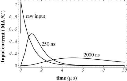
Figure 7: Raw input current signal and the signal after triple RC filters with time constants of $0.25\,\mu\mbox{s}$ and $2.0\,\mu\mbox{s}$.

Figure 8: The peak signal current after a triple RC filter vs. the filter time constant

Let us look at the case of an all analog filter. In this case all filtering is done prior to digitizing and the only digital processing performed is interpolation. I will take the B A B AR TDR design (described in subsection 6.1). This has a charge sensitive preamp followed by a CR and then two RC filters. Together these give the equivalent of three RC filters, all with the corner frequency $f_{c}$. This has the transfer function

$$F(\omega)=\left(\frac{-j\omega_{c}}{\omega-j\omega_{c}}\right)^{3}.$$ (78)

The signal is

$$I(\omega)=\left(\frac{-j\omega_{s}}{\omega-j\omega_{s}}\right).$$ (79)

Figure 9: The Equivalent Noise Energy (electronic only) of a single sample at the peak after a triple RC filter versus the radial velocity of the filter corner ($1/RC$).

Figure 10: The efficiency vs. 1/RC for nominal background conditions.

The time dependence of the output signal is given by the inverse Fourier transform of their product. This integral can be done by contour integration. If the contour is completed by a semi-circle at infinity around the upper half plane (for $t>0$), the integral can be deduced from the residues at the poles $j\omega_{c}$ and $j\omega_{s}$. The result is

$$o(t)=\frac{\omega_{c}^{3}\omega_{s}}{(\omega_{s}-\omega_{c})^{3}}\left\{\left(\frac{(\omega_{s}-\omega_{c})^{2}}{2}t^{2}-(\omega_{s}-\omega_{c})t+1\right)e^{-\omega_{c}t}-e^{-\omega_{s}t}\right\}.$$ (80)

This is shown for several time constants in figure 8. The peak value vs. time constant is shown in figure 8. Since there are no poles in the lower half plane, the integral is $0$ for $t<0$.

Figure 11: The efficiency vs. 1/RC for low background conditions.

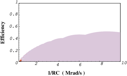
Figure 12: The efficiency vs. 1/RC for $10\times$ nominal background conditions.

The mean square noise is given by the inverse Fourier transform of the noise evaluated at $t=0$, i.e., the autocorrelation for no time difference. The noise before filtering is given by equation 51. The mean square noise is

$$n=\frac{1}{\pi}\int_{0}^{\infty}{N(\omega)|F(\omega)|^{2}\,d\omega}.$$ (81)

The contribution of the electronic noise is

$$n_{elec}=\omega_{c}(V_{n}^{2}C^{2}\omega_{c}^{2}+3I_{n}^{2})/32.$$ (82)

The peak of $\sqrt{n_{elec}/o^{2}(t)}$ gives the ENC for the electronic noise after analog filtering. Appropriate scaling gives the ENE shown in Figure 10. The background noise contribution is

$$n_{back}=\frac{(8\omega_{c}^{2}+9\omega_{s}\omega_{c}+3\omega_{s}^{2})\omega_{c}\omega_{s}I_{b}^{2}}{32(\omega_{c}+\omega_{s})^{3}}$$ (83)

$n$ is given by their sum. The signal to noise ratio for a single sample taken at time $t$ is given by $o^{2}(t)/n$. If we divide this by the optimum signal to noise given by equation 55 we get the “efficiency” for this single sample versus the sample time. Figure 10 shows this function for the B A B AR calorimeter during nominal operating conditions for several values of the corner frequency. The highest efficiency achieved is 68% for a shaping time constant of 0.2$\,\mu\mbox{s}$. For low background conditions (Figure 12) the peak efficiency is 80% at a shaping time of 1.5$\,\mu\mbox{s}$. At ten times nominal background, (Figure 12) the efficiency drops to 50% at a shaping time of 0.12$\,\mu\mbox{s}$. The loss of efficiency for nominal and better background conditions is not significant. The loss at during high background conditions hits just when noise is the causing the most problems. Matched filters utilize knowledge of the signal shape. In low background conditions, the optimum shaping time is longer than the signal. The shape of the signal is not seen and matched filters offer little advantage. The situation and conclusions are reversed in high background conditions.

The cost of using an analog filter optimized for conditions other than those encountered is more dramatic. If the corner frequency is set to the 0.2$\,\mu\mbox{s}$ which is optimal for nominal conditions, but the backgrounds are actually at $10\times$ nominal levels, the efficiency is 44%. If the corner frequency were optimal for low background conditions, the efficiency at $10\times$ nominal background would be 12%.

10 Summary of Significant Findings

Since the important conclusions may have gotten lost in the derivations, I’ll review them here.

• Machine background can be treated as a current noise with the spectrum of the signal.

• The best possible amplitude and time measurements can be obtained with a matched filter.

• The errors in the amplitude and time are not correlated, therefore knowing the time does not improve the ultimate precision of the amplitude determination, although such knowledge may reduce the computation required.

• The signal to noise methodology used here reproduces previous results.

• The background current noise dominates the photodiode shot noise even at nominal backgrounds and in the quietest part of the calorimeter.

• For nominal background where $I_{b}\gg I_{n}$:

  $$ENC^{2} \approx I_{b}^{2}\sqrt{2\tau_{s}\tau_{b}+\tau_{b}^{2}}=\sqrt{2\tau_{s}I_{b}^{3}V_{n}C+I_{b}^{2}V_{n}^{2}C^{2}}$$

  $$ENTC^{2} \approx ENC^{2}\tau_{s}\tau_{b}=\sqrt{2I_{b}\tau_{s}^{3}V_{n}^{3}C^{3}+\tau_{s}^{2}V_{n}^{4}C^{4}}$$

• The sampling frequency of 3.7 MHz is adequate at nominal backgraounds, but it is marginal for $10\times$nominal background levels.

• At this frequency, 64 samples will have to be processed under nominal conditions.

• The step of an ADC bit (on the most sensitive range) should be set so that there are at least 13 bits to full scale (12 GeV) during nominal background. For quiet conditions and with a differentiating stage in the analog filter, 16.5 bits may be required.

• Simple analog filters can achieve near optimal results in low to moderate background conditions if the shaping time is optimized for the actual conditions.

11 Acknowledgements

I thank my BaBar colleagues for consultations and for providing the data used in the examples. This work was supported by the U.S. Department of Energy under contract number DE-AC02-76SF00515.

References

- [Ambrozny] A. Ambrózny, Electronics Noise (McGraw-Hill, NY, NY, 1982).
- [BaBar] B A B AR Collaboration, Technical Design Report, SLAC-R-95-457, March 1995.
- [Bracewell] R. Bracewell, The Fourier Transform and Its Applications (McGraw-Hill, NY, NY, 1978).
- [Dow] S. Dow,et al., A CMOS Front End for the CsI(Tl)Calorimeter, B A B AR Note # 139 (1994).
- [Dwight] H. Dwight, Tables of Integrals and Other Mathematical Data (MacMillan, NY, NY, 1961).
- [Haller] D. Haller, D. Freytag, and J. Hoeflich, Proposal for the Electronics System for the B A B ARCsI(Tl)Calorimeter B A B AR Note # 184 (1994).
- [Humphreys] D. Humphreys, The Analysis, Design, and Synthesis of Electrical Filters (Prentice-Hall, Englewood Cliffs, NJ, 1970).
- [Maple] B. Char, et al., Maple V release 3, A symbolic algebra program. Maple is the trademark of Waterloo Maple Software.
- [Marsiske] H. Marsiske, private communication. This background calculation dates from April 1996. It includes modified beam optics and the expected vacuum profile. The lost particle background is calculated. This is then scaled up by a factor of 1.5 in the barrel and 2.0 in the endcap to account radiative Bhabha induced background.
- [Papoulis] A. Papoulis, Signal Analysis (McGraw-Hill, NY, NY, 1977).
- [Prudnikov] A. Prudnikov, Yu. Brychov, and O. Marichev Integrals and Series, Vol.I (, , , 19).
- [Radeka] V. Radeka, High Resolution Liquid Argon Total Absorption Detectors: Electronic Noise and Electrode Configuration, IEEE Trans.Nucl.Sci.Ns24 (1977) 293.
- [Skolnik] M. Skolnik, Radar Handbook (McGraw-Hill, NY, NY, 1970).
- [vanderZiel] A. van der Ziel, Noise in Solid State Devices and Circuits (Wiley, NY, NY, 1986).