Quasiparticle and quasihole states of nuclei around ⁵⁶Ni

Abstract

The single-particle spectral function of ⁵⁶Ni has been computed within the framework of self-consistent Green’s functions theory. The Faddeev random phase approximation method and the G-matrix technique are used to account for the effects of long- and short-range physics on the spectral distribution. Large scale calculations have been performed in spaces including up to ten oscillator shells. The chiral N³LO interaction is used together with a monopole correction that accounts for eventual missing three-nucleon forces. The single-particle energies associated with nucleon transfer to valence $1p0f$ orbits are found to be almost converged with respect to both the size of the model space and the oscillator frequency. The results support that ⁵⁶Ni is a good doubly magic nucleus. The absolute spectroscopic factors to the valence states on $A=55,57$ are also obtained. For the transition between the ground states of ⁵⁷Ni and ⁵⁶Ni, the calculations nicely agree with heavy-ion knockout experiments.

I Introduction

The way shell closures and single-particle energies evolve as functions of the number of nucleons is presently one of the greatest challenges to our understanding of the basic features of nuclei. Doubly-magic nuclei are particularly important and closed shell nuclei like ⁵⁶Ni and ¹⁰⁰Sn have been the focus of several experiments during the last years ni56a ; Yur.06 ; ni56c ; ni56d ; ni56e ; ni56f ; sn100a . Their structure provides important information on theoretical interpretations and our basic understanding of matter. In particular, recent experiments ni56a ; Yur.06 ; ni56c ; ni56d ; ni56e ; ni56f have aimed at extracting information about single-particle degrees of freedom in the vicinity of ⁵⁶Ni. Experimental information from single-nucleon transfer reactions and magnetic moments ni56a ; Yur.06 ; ni56c ; ni56d ; ni56f , can be used to extract and interpret complicated many-body wave functions in terms effective single-particle degrees of freedom. Transfer reactions provide for example information about the angular distributions, the excitation energies and the spectroscopic factors of possible single-particles states. If one can infer from experimental data that a single-particle picture is a viable starting point for interpreting a closed-shell nucleus like ⁵⁶Ni, one can use this nucleus as a basis for constructing valence-space effective interactions. These interactions can in turn be used in shell-model calculations of nuclei with several valence nucleons above the $N=28$ and $Z=28$ filled shells of ⁵⁶Ni. Recent measurements of spectroscopic factors of ⁵⁷Ni in high-energy knockout reactions Yur.06 seem to indicate that low-lying states in ⁵⁷Ni can be characterized as single-particle states on top of ⁵⁶Ni as a closed-core nucleus. Large-scale shell-model calculations by Horoi et al horoi2006 corroborate these findings, whereas a recent experiment on magnetic moments of the ground state of ⁵⁷Cu ni56f , expected to be described as one valence proton outside ⁵⁶Ni, resulted in much smaller moments than those expected from a single-particle picture. Similarly, large transition matrix elements between the $0_{1}^{+}$ ground state and the first excited $2_{1}^{+}$ state indicate that the ⁵⁶Ni core is rather soft ni56e , or stated differently, it implies a rather fragmented single-particle picture. On the other hand, one ought keep in mind that quenchings of spectroscopic factors to about 60% are common even for good closed shell nuclei lap93 . Experimentally, spectroscopic factors are defined as the ratio of the observed reaction rate with respect to the same rate calculated assuming a full occupation of the relevant single-particle states. They are therefore often interpreted as a measure of the occupancy of a specific single-particle state. However, from a strict theoretical point of view spectroscopic factors are not occupation numbers but a measure of what fraction of the full wave function can be factorized into a correlated state (often chosen to be a given closed-shell core) and an independent single-particle or single-hole state. Large deviations from the values predicted by an independent-particle model, point to a strongly correlated system. In this regime, collective excitations that behave like single-particle degrees of freedom—that is quasiparticles—can still arise.

The above mentioned large-scale shell-model calculations horoi2006 have been performed in one major shell, the $1p0f$-shell, with an effective interaction fitted to reproduce properties of several nuclei that can be interpreted in terms of these single-particle states. The number of possible Slater determinants that can be constructed when distributing eight valence protons and eight valence nucleons in the $1p0f$ shell is more than $10^{9}$. This means that the inclusion of more complicated particle-hole excitations from shells below and above the $1p0f$ shell, are well beyond present capabilities of large-scale diagonalization methods Whitehead1977 ; caurier2005 ; dean2004b ; navratil2004 ; horoi2006 . The hope is that an effective interaction tailored to one major shell includes as many as possible of these neglected particle-hole excitations. However, there are other many-body methods that allow for a computational scheme which accounts for a systematic inclusion of more complicated many-body corrections. Typical examples of such many-body methods are coupled-cluster methods bartlett2007 ; helgaker ; dean2004 ; Hag.08 , various types of Monte Carlo methods pudliner1997 ; kdl97 ; utsuno1999 , perturbative many-body expansions ellis1977 ; Hjo.95 , self-consistent Green’s functions (SCGF) methods DicVan ; Dic.04 ; vanneck2002 ; vanneck2003 ; vanneck2005 ; Bar.01 ; Bar.02 ; Bar.03 ; Bar.06 , the density-matrix renormalization group white1992 ; schollwock2005 ; dukelsky2002a ; pittel2006 and ab initio density functional theory bartlett2005 ; vanneck2006 , just to mention some of the available methods.

The Green’s function Monte Carlo method pudliner1997 ; pieper2001 ; wiringa2002 ; pieper2004 and the no-core shell-model approach navratil2004 ; navratil1998 ; navratil2000a ; navratil2002 ; navratil2000b ; navratil2003 ; nogga2006 have been successfully applied to the theoretical description of light nuclei with mass numbers $A\leq 12$, and Hamiltonians based on nucleon-nucleon and three-nucleon interactions. However, present experimental studies of nuclear stabilities are now being pushed to larger mass regions, with mass numbers from $A=40$ to $A=100$. Traditionally, this has been the realm of the nuclear shell-model and nuclear density-functional theory. These methods employ Hamiltonians and density functionals with phenomenological corrections and are not directly related to the vacuum nucleon-nucleon interaction employed in ab initio calculations (exceptions are found when perturbative many-body methods are used Hjo.95 ). However, in selected medium-mass nuclei, ab initio structure calculations can be performed using approaches like coupled-cluster and Green’s functions theories. These methods allow studying ground- and excited-state properties of systems with dimensionalities beyond the capability of present large-scale diagonalization approaches, with a much smaller numerical effort when compared to diagonalization methods aiming at similar accuracies. The accuracy of these methods is sufficiently high to attribute an eventual disagreement between experimental data and theoretical results to missing physics in the Hamiltonian. In this way, such calculations help to increase our understanding of the nuclear interaction on a very fundamental level.

Recent coupled-cluster calculations Hag.08 have reported practically converged results of the ground state of medium-mass nuclei like ⁴⁰Ca, ⁴⁸Ni and ⁴⁸Ca using the bare chiral interaction N³LO Ent.03 . These calculations employed a harmonic oscillator basis to construct the single-particle basis and included correlations of the so-called singles and doubles types. It means that one-particle-one-hole and two-particle-two-hole correlations acting on a many-body Slater determinant were summed to infinite order. Recently, results with three-particle-three-hole correlations have also been obtained hagen2009 . The calculations were performed in a harmonic oscillator basis containing up to fifteen major shells and resulted in basically converged ground state properties for a given Hamiltonian.

Another method with a strong potential for performing ab initio calculations of nuclei beyond $A=12$ is self-consistent Green’s functions theory. Differently from the coupled-cluster and no-core shell model, this method does not construct the wave function but evaluates directly the energies and transition matrix elements for the transfer of one or more nucleons. Another important point is that the self-energy–the central component of the formalism–has been shown to be an exact optical potential. On the one hand, one can employ the formalism for pure ab initio studies. On the other, the strong link with the response to experimental probes can be used to constrain and improve phenomenological models. An example of this approach is the dispersive optical model recently derived for chain of calcium isotopes Cha.06 ; Cha.07 . This global optical potential reproduces with high accuracy the known elastic scattering data, up to energies of 200 MeV. Thus, Green’s functions hold a promise of both bridging nuclear structure and reactions and for connecting the (relatively few) isotopes amenable of ab initio calculations to the rest of the nuclear landscape.

In practical applications of Green’s functions theory, one expands the self-energy in terms of resummations of Feynman diagrams and truncates the series in a way that allows for further systematic improvements of the formalism. A powerful scheme for non-perturbative expansions is the so called Faddeev random phase approximation (FRPA) that explicitly accounts for particle-vibration couplings Bar.01 ; Bar.07 . First applications of this approach were devoted to ¹⁶O. One single calculation yielded the basic information to be used for microscopic studies of spectroscopic factors Bar.02 ; Bar.09b , the excitation spectrum Bar.03 , two-nucleon emission Bar.04 ; Mid.06 and the nucleon-nucleus optical potential Bar.05 . Thus, the FRPA method pursues a global description of the many-body dynamics, far beyond ground state properties alone. Another difference with the coupled-cluster approach is that Green’s functions allow, via a diagrammatic approach, to directly introduce the correlations outside the model space that are associated with short-range degrees of freedom Mut.95 ; Geu.96 . It can therefore be applied to interactions with strong short-range cores (for example, the Argonne model Wir.95 was employed in Ref. Bar.06 ).

Self-consistent FRPA calculations of ¹⁶O were first performed by the authors of Ref. Bar.02 , and subsequently extended to fully ab initio calculations in spaces up to eight oscillator shells Bar.06 . To our knowledge, the combination of the random phase approximation phonons and the proper treatment of the energy dependence of the interaction vertex, makes this the most accurate evaluation of single-particle states available for this nucleus. In this work we extend the range of applications of this formalism to studies of quasiparticle states around ⁵⁶Ni, as a first application of Faddeev random phase approximation to $1p0f$ shell nuclei. As mentioned above, there is quite some experimental interest in single-particle properties around ⁵⁶Ni.

This work is organized as follows. Sec. II reviews the Faddeev random phase approximation approach and discusses the approximations made to calculate the self-consistent propagator. The convergence of single-particle properties is discussed in Sec. III and the results for the spectral function are described in Sec. IV. We refer the reader directly interested to discussion of physics results to the latter section. Conclusions are drawn in Sec. V.

II Formalism

This section serves as an overview of the formalism we employ. The treatment of short-range physics and the implementation of self-consistency, which are improved with respect to previous works, are discussed in details. The Faddeev random phase approximation expansion is also introduced, but we refer the reader for more details in Refs. Bar.01 ; Bar.07 .

In the framework of Green’s function theory, the object of interest is the single-particle propagator, instead of the many-body wave function. In the following, greek indices $\alpha,\beta,\dots$ label the orthonormal basis set of single-particle states included in the model space, while latin indices $k,l,\dots$ refer to many-body states. We employ the convention of summing over repeated indices, unless specified otherwise. The single-particle propagator can be written in the so-called Lehmann representation as FetWal ; DicVan

$$g_{\alpha\beta}(\omega)~{}=~{}\sum_{n}\frac{\left({\cal X}^{n}_{\alpha}\right)^{*}\;{\cal X}^{n}_{\beta}}{\omega-\varepsilon^{+}_{n}+i\eta}~{}+~{}\sum_{k}\frac{{\cal Y}^{k}_{\alpha}\;\left({\cal Y}^{k}_{\beta}\right)^{*}}{\omega-\varepsilon^{-}_{k}-i\eta}\;,$$ (1)

where ${\cal X}^{n}_{\alpha}={\mbox{$\langle{\Psi^{A+1}_{n}}|$}}c^{{\dagger}}_{\alpha}{\mbox{$|{\Psi^{A}_{0}}\rangle$}}$  (${\cal Y}^{k}_{\alpha}={\mbox{$\langle{\Psi^{A-1}_{k}}|$}}c_{\alpha}{\mbox{$|{\Psi^{A}_{0}}\rangle$}}$) are the spectroscopic amplitudes, $c_{\alpha}$ ($c^{\dagger}_{\alpha}$) are the second quantization annihilation (creation) operators and $\varepsilon^{+}_{n}=E^{A+1}_{n}-E^{A}_{0}$ ($\varepsilon^{-}_{k}=E^{A}_{0}-E^{A-1}_{k}$). With these definitions, $|\Psi^{A+1}_{n}\rangle$ and $|\Psi^{A-1}_{k}\rangle$ are the eigenstates, while $E^{A+1}_{n}$ and $E^{A-1}_{k}$ are the corresponding energies of the ($A\pm 1$)-nucleon system. Therefore, the poles of the single-particle propagator reflect the energy transfer observed in pickup and knockout reactions.

The single-particle propagator $g_{\alpha\beta}(\omega)$ enters the Dyson equation as

$$g_{\alpha\beta}(\omega)=g^{0}_{\alpha\beta}(\omega)\;+\;g^{0}_{\alpha\gamma}(\omega)\Sigma^{\star}_{\gamma\delta}(\omega)g_{\delta\beta}(\omega)\;.$$ (2)

It depends on the irreducible self-energy $\Sigma^{\star}(\omega)$. The latter can be written as the sum of two terms. The first terms describes the average mean-field (MF) while the second term contains dynamic correlations,

$$\Sigma^{\star}_{\alpha\beta}(\omega)~{}=~{}\Sigma^{MF}_{\alpha\beta}~{}+~{}\frac{1}{4}\,V_{\alpha\lambda,\mu\nu}~{}R_{\mu\nu\lambda,\gamma\delta\varepsilon}(\omega)~{}V_{\gamma\delta,\beta\varepsilon}\;.$$ (3)

In Eq. (2), $g^{0}(\omega)$ is the so-called unperturbed single-propagator, corresponding to nucleons moving under the effect of the kinetic energy part of the total Hamiltonian. The localization of the single-particle states in the nuclear mean-field is due to the term $\Sigma^{MF}$, which extends the Hartree-Fock potential to that of a fully correlated density matrix. The term $V_{\alpha\beta,\gamma\delta}$ represents the antisymmetrized matrix elements of the nucleon-nucleon interaction. In this work, these will be approximated by an effective interaction, Eq. (8), discussed in Sec. II.1. Eq. (3) introduces the two-particle-one-hole (2p1h) and two-hole-one-particle (2h1p) irreducible propagator $R(\omega)$. In its Feynman expansion, this propagator contains all diagrams with any number of particle and hole lines except those that allow the intermediate propagation of one single line. It can therefore be interpreted as carrying the complete information on all configurations that cannot be reduced to a nucleon interacting with the average nuclear field. In particular, it includes the coupling of single-particle states to collective vibrations like giant resonances.

The theoretical spectroscopic factors $Z_{k}$ and $Z_{n}$ for removal and addition, respectively, of a nucleon, are given by the normalization integral of the corresponding overlap wave functions. In the notation of Eq. (1), these are

$$Z_{k} = \sum_{\alpha}\left|\langle{\Psi^{A-1}_{k}}|c_{\alpha}|{\Psi^{A}_{0}}\rangle\right|^{2}=\sum_{\alpha}\left|{\cal Y}^{k}_{\alpha}\right|^{2}\;,$$

$$Z_{n} = \sum_{\alpha}\left|\langle{\Psi^{A+1}_{n}}|c^{{\dagger}}_{\alpha}|{\Psi^{A}_{0}}\rangle\right|^{2}=\sum_{\alpha}\left|{\cal X}^{n}_{\alpha}\right|^{2}\;.$$ (4)

The hole states are normalized according to

$$Z_{k}=\sum_{\alpha}\left|{\cal Y}^{k}_{\alpha}\right|^{2}=1+\sum_{\alpha,\beta}\left({\cal Y}^{k}_{\alpha}\right)^{*}\left.\frac{\partial\Sigma^{*}_{\alpha\beta}(\omega)}{\partial\omega}\right|_{\omega=\varepsilon^{-}_{k}}{\cal Y}^{k}_{\beta}\;\;,$$ (5)

which follows directly from the Dyson equation (2). The same relation applies to particle states, with ${\cal Y}^{k}_{\alpha}$ replaced by $\left({\cal X}^{n}_{\alpha}\right)^{*}$. Because of the analytical properties of $\Sigma^{\star}(\omega)$, the derivative term results always in a negative contribution, leading thereby to a quenching of the spectroscopic factors.

It must be stressed that Eqs. (2) and (3) do not involve any approximation. Therefore, the full knowledge of $\Sigma^{MF}$ and $R(\omega)$ would be equivalent to the exact solution of the Schrödinger equation. In practical calculations, it is always necessary to truncate the full space of available single-particle states to a finite model space and to select a limited set of many-body correlations. The approximations employed in the present work to evaluate these quantities are discussed in the rest of this section.

II.1 Short-range physics and effective interaction

The present calculations were performed within a large but finite set of harmonic oscillator states, including single-particle states up to ten major shells. In order to treat the short-range part of the nucleon-nucleon interaction, one must resum explicitly the series of ladder diagrams for two nucleons outside this model space. These contributions are included in the self-energy in two different ways. Firstly, they are explicitly added to the mean-field part, $\Sigma^{MF}$, in order to reconstruct the contribution of short-range correlations in the full Hilbert space. Secondly, they are included in a regularized effective Hamiltonian which is used to calculate the long-range part of correlations—described by $R(\omega)$—inside the chosen model space. This approach leads to calculating the well known $G$-matrix Hjo.95 ; CENS.08 , which is then used as an energy dependent effective interaction inside the model space . In this case the $\Sigma^{MF}$ part of the self-energy will also depend on energy. This is given by

$$\Sigma^{MF}_{\alpha\beta}(\omega) = i\sum_{\gamma\delta}\int\frac{d\omega^{\prime}}{2\pi}G_{\alpha\gamma,\delta\beta}(\omega+\omega^{\prime})g_{\gamma\delta}(\omega^{\prime})$$ (6)

$$= \sum_{\gamma\delta}\sum_{k}G_{\alpha\gamma,\beta\delta}(\omega+\varepsilon^{-}_{k})\;{\cal Y}^{k}_{\delta}\;\left({\cal Y}^{k}_{\gamma}\right)^{*}\;,$$

where $G_{\alpha\beta,\gamma\delta}(\omega)$ are the matrix elements of the $G$-matrix interaction. Eq. (6) differs from the standard Brueckner-Hartree-Fock potential in the fact that the mean-field is not represented by a set of independent nucleons filling various orbits. Rather, the medium is described by the hole spectroscopic amplitudes ${\cal Y}^{k}$ that lead to the fully correlated density matrix. Since the latter are obtained by solving the Dyson equation, they must be obtained iteratively in a self-consistent way. Whenever the second term in Eq. (3) is neglected, this procedure simply reduces to solving the standard Brueckner-Hartree-Fock equations. However, as soon as the response of the medium $R(\omega)$ is accounted for, the single-particle propagator becomes fragmented and $\Sigma^{MF}$ describes the interaction of a particle with the “correlated” medium.

We remind that using the $G$-matrix in Eq. (6) corresponds to summing the mean-field term form Eq. (3) and ladder diagrams with intermediate two-particle states outside the chosen model space. This partitioning procedure has two main consequences. First, the effects of short-range physics at the two-body level on the total energy are included in the renormalized interaction. This leads to a softer force that can be applied within a “low-momentum” model space. Secondly, due to the explicit energy dependence, the term $\Sigma^{MF}(\omega)$ contributes as well to the normalization of spectroscopic factors, Eq. (5). This provides a natural way to determine the amount of strength that the free interaction would admix into configurations outside the model space, see for example the discussion of Refs. Mut.95 ; Geu.96 . Thus, the present approach differs from methods based on the renormalization group, where instead an explicit renormalization of the effective operators would be required Ste.05 .

The energy dependence of the $G$-matrix becomes cumbersome in calculating the polarization propagator. We define therefore a static effective interaction for our model space to be used in our calculations of the second term on the right-hand side of Eq. (3). To do this we evaluate the average energy for the harmonic oscillator single-particle states according to

$$\varepsilon^{ho}_{\alpha}=\langle\alpha|\frac{p^{2}}{2m}|\alpha\rangle~{}+~{}\sum_{\beta\in F}G_{\alpha\beta,\alpha\beta}(\omega=\varepsilon^{ho}_{\alpha}+\varepsilon^{ho}_{\beta})\;,$$ (7)

where the sum is limited to those states that correspond to filled orbits in the independent particle model. Note that in Eq. (7) the single-particle energies are derived iteratively while the oscillator wave functions remain unchanged. Clearly, these orbits are a crude approximation to the real quasiparticle states and will not be used to construct $R(\omega)$ in Sec. II.2–which will be rather determined in a self-consistent fashion. The main purpose of the above procedure is to yield a prescription for obtaining a starting energy independent effective interaction. Following Gad and Müther Gad.02 , we use the single-particle energies from Eq. (7) to define an interaction for the given model space by

$$V_{\alpha\beta,\gamma\delta}=\frac{1}{2}[G_{\alpha\beta,\gamma\delta}(\omega=\varepsilon^{ho}_{\alpha}+\varepsilon^{ho}_{\beta})~{}+~{}G_{\alpha\beta,\gamma\delta}(\omega=\varepsilon^{ho}_{\gamma}+\varepsilon^{ho}_{\delta})]\;.$$ (8)

The $G$-matrix can be computed according Ref. Hjo.95 ; CENS.08 for negative energies, up to about $-5$ MeV. For larger values we fix the starting energy to $\omega=-5$ MeV. Note that the starting energy appearing in Eq. (6) is shifted by the quasihole poles $\varepsilon^{-}_{k}$. This ensures that the energy dependence of $\Sigma^{MF}(\omega)$ is fully accounted for all quasiparticle states in the $1p0f$ shell.

II.2 The Faddeev random phase approximation method

The polarization propagator $R(\omega)$ can be expanded in terms of simpler Green’s functions that involve the propagation of one or more quasiparticle states. This approach has the advantage that it aids in identifying key physics ingredients of the many-body dynamics. By truncating the expansion to a particular subsets of diagrams or many-body correlations, one can then construct suitable approximations to the self-energy. Moreover, since infinite sets of linked diagrams are summed the approach is non-perturbative and satisfies the extensivity condition bartlett2007 . This expansion also serves as a guideline for systematic improvements of the method.

Following Refs. Bar.01 ; Bar.07 , we first consider the particle-hole polarization propagator that describes excited states in the $A$-particle system

$$\Pi_{\alpha\beta,\gamma\delta}(\omega) = \sum_{n\neq 0}\frac{{\mbox{$\langle{\Psi^{N}_{0}}|$}}c^{{\dagger}}_{\beta}c_{\alpha}{\mbox{$|{\Psi^{N}_{n}}\rangle$}}\;{\mbox{$\langle{\Psi^{N}_{n}}|$}}c^{{\dagger}}_{\gamma}c_{\delta}{\mbox{$|{\Psi^{N}_{0}}\rangle$}}}{\omega-\left(E^{N}_{n}-E^{N}_{0}\right)+i\eta}$$ (9)

$$- \sum_{n\neq 0}\frac{{\mbox{$\langle{\Psi^{N}_{0}}|$}}c^{{\dagger}}_{\gamma}c_{\delta}{\mbox{$|{\Psi^{N}_{n}}\rangle$}}\;{\mbox{$\langle{\Psi^{N}_{n}}|$}}c^{{\dagger}}_{\beta}c_{\alpha}{\mbox{$|{\Psi^{N}_{0}}\rangle$}}}{\omega+\left(E^{N}_{n}-E^{N}_{0}\right)-i\eta}\;,$$

and the two-particle propagator that describes the addition/removal of two particles

$$g^{II}_{\alpha\beta,\gamma\delta}(\omega) = \sum_{n}\frac{{\mbox{$\langle{\Psi^{N}_{0}}|$}}c_{\beta}c_{\alpha}{\mbox{$|{\Psi^{N+2}_{n}}\rangle$}}\;{\mbox{$\langle{\Psi^{N+2}_{n}}|$}}c^{{\dagger}}_{\gamma}c^{{\dagger}}_{\delta}{\mbox{$|{\Psi^{N}_{0}}\rangle$}}}{\omega-\left(E^{N+2}_{n}-E^{N}_{0}\right)+i\eta}$$ (10)

$$- \sum_{k}\frac{{\mbox{$\langle{\Psi^{N}_{0}}|$}}c^{{\dagger}}_{\gamma}c^{{\dagger}}_{\delta}{\mbox{$|{\Psi^{N-2}_{k}}\rangle$}}\;{\mbox{$\langle{\Psi^{N-2}_{k}}|$}}c_{\beta}c_{\alpha}{\mbox{$|{\Psi^{N}_{0}}\rangle$}}}{\omega-\left(E^{N}_{0}-E^{N-2}_{k}\right)-i\eta}\;.$$

These Green’s functions contain in their Lehmann representations all the relevant information regarding the excitation of particle-hole and two-particle or two-hole collective modes. In this work we are interested in studying the influence of giant resonance vibrations, which can be described within the random phase approximation (RPA). In the Faddeev RPA approach, the propagators of Eqs. (9) and (10) are then evaluated by solving the usual RPA equations, which are depicted diagrammatically in Fig. 1. Since these equations reflect two-body correlations, they still have to be coupled to an additional single-particle propagator, as in Fig. 2, to obtain the corresponding approximation for the two-particle-one-hole and two-hole-one-particle components of $R(\omega)$. This is achieved by solving two separate sets of Faddeev equations, as discussed in Ref. Bar.01 .

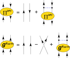
Figure 1: (Color online) Diagrammatic equations for the polarization (above) and the two-particle (below) propagators in the RPA approach. Dashed lines are matrix elements of the effective nucleon-nucleon interaction, Eq. (8). The full lines represent the independent-particle model propagator $g^{IPM}(\omega)$, which is employed instead of the fully dressed one. See the text for details.

Taking the two-particle-one-hole (2p1h) case as an example, one can split $R^{(2p1h)}(\omega)$ in three different components $\bar{R}^{(i)}(\omega)$ ($i=1,2,3$) that differ from each other by the last pair of lines that interact in their diagrammatic expansion,

$$\bar{R}^{(2p1h)}_{\alpha\beta\gamma,\mu\nu\lambda}(\omega)=\left[{G^{0}}^{>}_{\alpha\beta\gamma,\mu\nu\lambda}(\omega)-{G^{0}}^{>}_{\beta\alpha\gamma,\mu\nu\lambda}(\omega)\right]+\sum_{i=1,2,3}\bar{R}^{(i)}_{\alpha\beta\gamma,\mu\nu\lambda}(\omega)\;,$$ (11)

where ${G^{0}}^{>}(\omega)$ is the 2p1h propagator for three freely propagating lines. These components are solutions of the following set of Faddeev equations Fad.61

$$\bar{R}^{(i)}_{\alpha\beta\gamma,\mu\nu\lambda}(\omega)~{}=~{}{G^{0}}^{>}_{\alpha\beta\gamma,\mu^{\prime}\nu^{\prime}\lambda^{\prime}}(\omega)~{}\Gamma^{(i)}_{\mu^{\prime}\nu^{\prime}\lambda^{\prime},\mu^{\prime\prime}\nu^{\prime\prime}\lambda^{\prime\prime}}(\omega)$$

$$\times ~{}\left[\bar{R}^{(j)}_{\mu^{\prime\prime}\nu^{\prime\prime}\lambda^{\prime\prime},\mu\nu\lambda}(\omega)~{}+~{}\bar{R}^{(k)}_{\mu^{\prime\prime}\nu^{\prime\prime}\lambda^{\prime\prime},\mu\nu\lambda}(\omega)\right.$$

$$~{}~{}+~{}\left.{G^{0}}^{>}_{\mu^{\prime\prime}\nu^{\prime\prime}\lambda^{\prime\prime},\mu\nu\lambda}(\omega)-{G^{0}}^{>}_{\nu^{\prime\prime}\mu^{\prime\prime}\lambda^{\prime\prime},\mu\nu\lambda}(\omega)\right]\;,~{}~{}i=1,2,3~{}$$

where ($i,j,k$) are cyclic permutations of ($1,2,3$). The interaction vertices $\Gamma^{(i)}(\omega)$ contain the couplings of a particle-hole (ph), see Eq. (9), or two-particle/two-hole (pp/hh), see Eq. (10), collective excitations and a freely propagating line. The propagator $R(\omega)$ which we employ in Eq. (3) is finally obtained by

$$R^{(2p1h)}_{\alpha\beta\gamma,\mu\nu\lambda}(\omega)~{}=~{}U_{\alpha\beta\gamma,\mu^{\prime}\nu^{\prime}\lambda^{\prime}}\;\bar{R}^{(2p1h)}_{\mu^{\prime}\nu^{\prime}\lambda^{\prime},\mu^{\prime\prime}\nu^{\prime\prime}\lambda^{\prime\prime}}(\omega)\;U^{\dagger}_{\mu^{\prime\prime}\nu^{\prime\prime}\lambda^{\prime\prime},\mu\nu\lambda}\;,$$ (13)

where the matrix $U$ has the effect of renormalizing the strength of the dynamic self-energy. This correction ensures consistency with perturbation theory up to third order. The explicit formulae of the matrices $\Gamma^{(i)}(\omega)$ and $U$ are given in terms of the propagators of Eqs. (9), (10) and (14), and the interaction $V_{\alpha\beta,\gamma\delta}$. They are discussed in detail in Ref. Bar.07 . The calculation of the 2h1p component of $R(\omega)$ follows completely analogous steps.

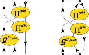
Figure 2: (Color online) Example of one of the diagrams that are summed to all orders by means of the Faddeev random phase approximation Eqs. (II.2) (left). The corresponding contribution to the self-energy, obtained upon insertion into Eq. (3), is also shown (right).

The present formalism includes the effects of ph and pp/hh motion simultaneously, while allowing interferences between these modes. These excitations are evaluated here at the RPA level and are then coupled to each other by solving Eqs. (II.2). This generates diagrams as the one displayed in Fig. 2. The Faddeev equations also ensure that the Pauli principle is correctly taken into account at the 2p1h and 2h1p level. In addition, one can in principle employ dressed single-particle propagators in these equations to generate a fully self-consistent solution, as done in Refs. Bar.02 ; Bar.06 for valence orbits around ¹⁶O.

II.3 Self-consistent approach

In the self-consistent Green’s function approach, both the $\Sigma^{MF}$ part of the self-energy and the polarization propagator $R(\omega)$ are expressed directly in terms of the exact single-particle propagator $g(\omega)$. The lines in Figs. 1 and 2 should thus represent the fully dressed propagator obtained by solving the Dyson equation. Since the degrees of freedom contained in Eq. (1) are excitations of the fully correlated system, the formalism does not depend on an explicit reference state. Normally, one first computes Eq. (3) in terms of an approximate propagator. The solution of Eq. (2) is then used to calculate an improved self-energy and the procedure is iterated to convergence. Baym and Kadanoff have shown that the self-consistency requirement implies the conservation of both microscopic and macroscopic properties Bay.61 ; Bay.62 . Intuitively, the self-consistency requirement becomes important whenever dynamical correlations modify substantially the response with respect to the Hartree-Fock mean-field (an example is the band-gap error problem in diamond crystals Oni.02 ). When applying standard Hartree-Fock theory to nuclear structure, most realistic interactions predict unbound nuclei and valence orbits in the continuum. This is a very poor starting point for any application of perturbation theory and other many-body techniques. However, the self-consistent approach requires using correlated quasiparticle energies and wave functions [the poles and residues of Eq. (1)]. These degrees of freedom form an optimal starting point for studies of many-body dynamics at the Fermi surface.

Accounting for the fragmentation of the single-particle propagator in the Faddeev random phase approximation increases the computational load as one moves to larger nuclei and model spaces. In this situation it is convenient to expand $R(\omega)$ in terms of an independent-particle model (IPM) propagator. This should approximate the dressed one but with a limited number of poles. Thus, we solve Eq. (II.2) in terms of

$$g^{IPM}_{\alpha\beta}(\omega)~{}=~{}\sum_{n/\in F}\frac{\left(\phi^{n}_{\alpha}\right)^{*}\;\phi^{n}_{\beta}}{\omega-\varepsilon^{IMP}_{n}+i\eta}~{}+~{}\sum_{k\in F}\frac{\phi^{k}_{\alpha}\;\left(\phi^{k}_{\beta}\right)^{*}}{\omega-\varepsilon^{IMP}_{k}-i\eta}\;,$$ (14)

where $F$ represent the set of occupied orbits. The single-particle energies $\varepsilon^{IPM}$ and wave functions $\phi$ are chosen such that $g^{IPM}(\omega)$ coincides with the real propagator $g(\omega)$ at the Fermi surface. To do this we define the following moments of the poles of Eq. (1).

$$M^{p}_{\alpha\beta}=\sum_{n}\frac{\left({\cal X}^{n}_{\alpha}\right)^{*}\;{\cal X}^{n}_{\beta}}{\left[E_{F}-\varepsilon^{+}_{n}\right]^{p}}+\sum_{k}\frac{{\cal Y}^{k}_{\alpha}\;\left({\cal Y}^{k}_{\beta}\right)^{*}}{\left[E_{F}-\varepsilon^{-}_{k}\right]^{p}}\;,~{}~{}p=0,1,2,\ldots$$ (15)

where $E_{F}$ is the Fermi energy. Eq. (14) is determined by imposing $M^{0,IPM}_{\alpha\beta}=M^{0}_{\alpha\beta}$ and $M^{1,IPM}_{\alpha\beta}=M^{1}_{\alpha\beta}$. The purpose of Eq. (15) is to define a set of effective single-particle orbits and energies that conserve the total spectroscopic strength carried by the self-consistent propagator and the centroids of its fragmented states. While effective single-particle properties form an appropriate starting point to evaluate $R(\omega)$, it remains clear that they only represent average quantities. Instead, it is Eq. (1) that must be related to experiment.

The propagator $g^{IPM}(\omega)$ is derived from Eq. (1) and it still needs to be evaluated in a iterative way. Therefore, the resulting propagator $R(\omega)$ is (partially) self-consistent. We stress that Eq. (6) can be calculated easily from the fully dressed propagator. Thus self-consistency is achieved exactly at the mean-field level.

III Calculations and convergence

The present calculations were performed using a harmonic oscillator basis and including up to ten major harmonic oscillator shells. We label these spaces with $N_{max}=3$, 5, 7, or 9, where $N=2n+l$. For the largest model space employed, $N_{max}=9$, all partial waves with orbital angular momentum $l\leq 7$ were included. This amount to 368 single-particle states for each particle species, protons and neutrons in our case. The total number of available Slater determinants for ⁵⁶Ni without any particular restrictions is proportional to the product of the two binomials

$$\left(\begin{array}[]{c}368\\ 28\end{array}\right)\times\left(\begin{array}[]{c}368\\ 28\end{array}\right),$$

a number which clearly exceeds the capabilities of any direct large-scale diagonalization procedure.

The codes utilize a $jj$-coupling scheme to decouple the Faddeev equations of Eq. (II.2). At each iteration, the RPA equations are solved in the particle-hole and the particle-particle and hole-hole channels using the single-particle orbits and energies from Eq. (14). The resulting propagators are inserted in Eqs. (II.2), which in turn are casted into a non Hermitian eigenvalue problem Bar.01 . In our largest calculation we diagonalize dense matrices of dimension up to $26\times 10^{3}$ two-particle-one-hole states. This number is bound to increase when larger nuclei are investigated or more details of nuclear fragmentation (that is more poles) are included in $g^{IPM}(\omega)$ (14). The numerical implementation of the Faddeev random phase approximation required careful optimization in evaluating the elements of the Faddeev matrix and a proper generalization of the Arnoldi algorithm anrref to employ multiple pivots. Similar improvements allowed to extend large scale calculations from the $A=16$ mass region to the $A=56$ mass region. The dimensions reached in this work represent roughly the upper limit when using table top single processor computers. Obviously, there is much to gain by taking advantage of modern supercomputer facilities and future research efforts should be put into parallelization of the present algorithms.

Model spaces of eight to ten major shells are large enough for a proper description of the response due to long-range correlations. These include excitations of several MeVs into the region of giant resonances. The effects of short-range physics are also included by using a $G$-matrix and an effective interaction as discussed in Sec. II.1. These are derived using the chiral nucleon-nucleon interaction N³LO by Entem and Machleidt Ent.03 . This interaction employs a cutoff of $\Lambda=500$ MeV.

Typical realistic two-nucleon interactions fail in reproducing the spin-orbit splittings and gaps between different shells. In particular, for the $N=28$ and $Z=28$ subshell closures these lead to an underestimation of the gap at the Fermi surface. In these cases, a complete diagonalization of the Hamiltonian would predict a deformed ground state of these nuclei even when they are experimentally known to be good spherical closed-shells systems caurier2005 ; Hor.07 . This issue can be cured with a simple modification of the monopole strengths of the interaction. Recently, Zuker has reported that the same correction works well for several isotopes throughout the nuclear chart and proposed that this may be interpreted as a signature of missing three-nucleon interactions Zuk.03 .

The inclusion of three-nucleon interactions to the Faddeev random phase approximation formalism is beyond the scope of the present work. However, it will be shown in Sec. III.1 that properly reproducing the Fermi gap is crucial in order to obtain meaningful results for the valence space spectroscopic factors. Thus, we follow Ref. Zuk.03 and modify the monopoles in the N³LO interaction model as

$$\Delta V^{T}_{fr} \rightarrow \Delta V^{T}_{fr}-(-1)^{T}\kappa_{M}\;,$$

$$\Delta V^{T}_{ff} \rightarrow \Delta V^{T}_{ff}-1.5(1-T)\kappa_{M}\;,$$ (16)

where $f$ and $r$ stand for the Brueckner-Hartree-Fock states associated to the $0f_{7/2}$ and the ($1p_{3/2}$,$1p_{1/2}$,$0f_{5/2}$) orbits, respectively. In the limit of large spaces, the Brueckner-Hartree-Fock orbits converge to the Hartree-Fock states and this correction becomes independent of the choice of the single-particle basis. Note that the prescription of Eq. (16) modifies only a few crucial matrix elements while about six millions of them are defined in the $N_{max}=9$ model space.

We also note that the present truncation of the model space, in terms of the number of oscillator shells, does not separate exactly the center of mass motion. Coupled-cluster calculations have shown that the error introduced by this truncation becomes negligibly small for large model spaces such as the ones employed here and therefore it does not represent a major issue gour2006 ; Hag.08 . In calculations of binding energies, it customary to subtract the operator for the kinetic energy of the center of mass directly from the Hamiltonian. This term automatically corrects for the zero point motion in oscillator basis but it depends explicitly on the number of particles. In this work, we are interested in transitions to states with different numbers of nucleons [(A$\pm$1] and aim at computing directly the differences between the total energies. Therefore, the above correction should not be employed in the present case. One may note that the separation of the center-of-mass motion is an issue related to the choice made for the model space, rather than the many-body method itself. For example, expressing the propagators directly in momentum space would allow an exact separation. In this situation, the transformation between the center-of-mass and laboratory frames for systems with a nucleon plus a $A$ nucleons (or $(A-1)$ nucleons) core would also be simple.

III.1 Choice of $\kappa_{M}$

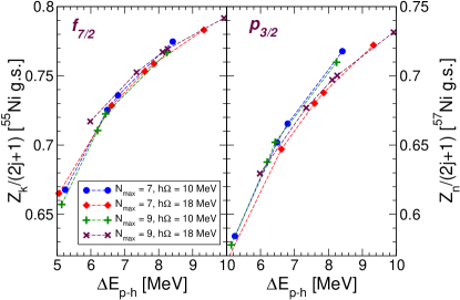
Figure 3: (Color online) Dependence of neutron spectroscopic factors (given as a fraction of the independent-particle model value) for the $1p_{3/2}$ and the $0f_{7/2}$ valence orbits with respect the ph gap $\Delta E_{ph}$. For each model space, different points correspond to different choices of $\kappa_{M}$ in the range $0.4-0.7$ MeV.

Eq. (16) introduces a single parameter ($\kappa_{M}$) in our calculations. The reason for this modification is that the spectroscopic factors of the valence orbits are strongly sensitive to the particle-hole gap. This sensitivity is to be expected since collective modes in the ⁵⁶Ni core are dominated by excitations across the Fermi surface. Smaller gaps imply lower excitation energies and higher probability of admixture with valence orbits. In order to extract meaningful predictions for spectroscopic factors it is therefore necessary to constrain the Fermi gaps for protons and neutrons to their experimental values.

To investigate this dependency we repeated our calculations for values of $\kappa_{M}$ in the range $0.4-0.7$ MeV. Fig. 3 shows the resulting neutron spectroscopic factors for the valence $p_{3/2}$ quasiparticle and $f_{7/2}$ quasihole. These are plotted as a function of the calculated particle-hole gap $\Delta E_{ph}=\varepsilon^{+}_{1p_{3/2},n=0}-\varepsilon^{-}_{0f_{7/2},k=0}$. The results correspond to model spaces of different dimensions (eight or ten oscillator shells) and oscillator frequencies ($\hbar\Omega=10$ or 18 MeV). The gap $\Delta E_{ph}$ increases with $\kappa_{M}$ but the dependence on the model space is weak. We notice that, once the experimental value of $\Delta E_{ph}$ is reproduced, the spectroscopic factors are well defined and found to be converged with respect to the given model space.

All results reported below were obtained with a fixed value of $\kappa_{M}=0.57$ MeV. In the $N_{max}=9$ model space and an oscillator energy $\hbar\Omega=10$  MeV, this choice reproduces the experimental gaps at the Fermi surface for both protons and neutrons to an error within $70$ keV. From Fig. 3 one infers that the calculated spectroscopic factors are reliable to within $1-2$% of the independent-particle model value.

III.2 Convergence with respect to choice of model space

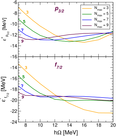
Figure 4: (Color online) Dependence of the neutron $1p_{3/2}$ particle energy and the $0f_{7/2}$ hole energy with respect to the oscillator frequency and the size of the model space.

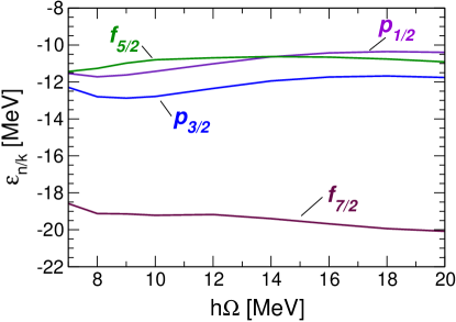
Figure 5: (Color online) Dependence of neutron single-particle energies on the oscillator frequency. The energies plotted here are the poles of $g(\omega)$ corresponding to the valence $1p0f$ orbits. Calculations were performed for $N_{max}=9$ and $l\leq 7$.

Fig. 4 shows the dependence of the neutron $1p_{3/2}$ particle and the $0f_{7/2}$ hole energies with respect to the oscillator frequency and the size of the model space. As can be seen from this figure, the single-particle energies for these two single-particle states tend to stabilize around eight to ten major shells. This finding concords both with coupled-cluster calculations that employ a $G$-matrix as effective interaction for ¹⁶O, see Refs. wloch2005 ; gour2006 , and with analogous Green’s functions studies Bar.06 . It remains however to make an extensive comparison between coupled-cluster theory and the Green’s function approach in order to find an optimal size of the model space with a given nucleon-nucleon interaction. Finally, we plot in Fig. 5 the neutron valence single-particle energies for all the single-particle states in $1p0f$-shell. The latter results were obtained with our largest model space, ten major shells with $N_{max}=9$ and the single-particle orbital momentum $l\leq 7$. As can be seen from this figure, there is still, although weak, a dependence upon the oscillator parameter. To perform calculations beyond ten major shells will require non trivial extensions of our codes.

IV Results for the spectral function

		$\varepsilon^{+}_{n}$, $\varepsilon^{-}_{k}$			$Z_{n}/(2j+1)$, $Z_{k}/(2j+1)$
		————————–			————————–
		FRPA	Exp.		FRPA	Exp.
57Ni:
$\nu 1p_{1/2}$		-11.43	-9.134		0.63
$\nu 0f_{5/2}$		-10.80	-9.478		0.59
$\nu 1p_{3/2}$		-12.78	-10.247		0.65	0.58(11)
55Ni:
$\nu 0f_{7/2}$		-19.22	-16.641		0.72
57Cu:
$\pi 1p_{1/2}$		-1.28	+0.417		0.66
$\pi 0f_{5/2}$		-0.58			0.60
$\pi 1p_{3/2}$		-2.54	-0.695		0.67
55Co:
$\pi 0f_{7/2}$		-9.08	-7.165		0.73

Table 1: Energies (in MeV) and spectroscopic factors (as a fraction of the independent-particle model) for transitions to the $1p0f$ valence orbits, obtained for $\hbar\Omega=10$ MeV, $N_{max}=9$ and $\kappa_{M}=0.57$ MeV. The experimental single-particle energies are taken from toi.96 . The measured spectroscopic factor for transfer between the ground states of ⁵⁷Ni and ⁵⁶Ni is from Ref. Yur.06 .

Our results for spectroscopic factors for the $1p0f$-shell valence orbits and the corresponding single-particle energies are collected in Table 1. In general, the modified N³LO interaction predicts single-particle energies about $2-3$ MeV lower than the experimental ones. The Coulomb shift between corresponding neutron and proton orbits is calculated to be about $10.2$ MeV and it is closer to the empirical value of $9.5$ MeV. For the oscillator parameter chosen, $\hbar\Omega=10$ MeV, we obtain an inversion of the $1p_{1/2}$ and $0f_{5/2}$ excited states in ⁵⁷Ni, with respect to the experiment. However, this discrepancy disappears for larger values of $\hbar\Omega$ (see Fig. 5). This effect is in fact smaller than the residual dependence on the model space and therefore no conclusion can be made about the ordering for the fully converged result. The spectroscopic factor for the transition between the ground states of ⁵⁷Ni and ⁵⁶Ni was extracted from high energy knockout reactions in Ref. Yur.06 . The self-consistent Faddeev random phase approximation result for this quantity yield 65% of the independent-particle model value, and agrees with the empirical data within experimental uncertainties. The theoretical spectroscopic factors for the excited states in ⁵⁷Ni are similar, with the $0f_{5/2}$ state being somewhat smaller, at about 59%. A larger value is obtained for knockout to the ground state of ⁵⁵Ni, which is predicted to be 72%. The results for proton transfer to particle (hole) states in ⁵⁷Cu (⁵⁵Co) are only slightly larger. According to the analysis of Fig. 3, it is expected that these predictions are converged within 1-2% of the independent-particle model values.

Past studies Gou.69 ; ni56e ; ni56f have questioned whether low-energy quasiparticle states in ⁵⁷Ni are strongly admixed to excitations of a soft ⁵⁶Ni core. The results obtained here do not suggest substantial differences with respect to other known closed shell nuclei. The spectroscopic factors from Table 1 are in line with observations from stable nuclei lap93 ; Gad.08 and support the hypothesis that ⁵⁶Ni is a good closed-shell nucleus. In our calculations we find that the $1p_{3/2}$ quasiparticle state of ⁵⁷Ni carries 65% of the strength for this orbit. Another 20% is located in the particle region below $\varepsilon^{+}_{n}$=2 MeV (above this energy strength associated with the $2p1f0h$ shell starts to appear), and about 3% is in the hole region above $\varepsilon^{-}_{k}=-40$ MeV (see Fig. 6). Similarly, the $0f_{7/2}$ state has 72% of the independent-particle model strength in the quasihole peak (the ground state of ⁵⁵Ni), 10% in the fragmented hole region, and 3% in the fragmented particle region. This analysis confirms that the main mechanism responsible for the quenching of the spectroscopic factors lies in the admixture between single-particle states and collective excitations in the region of giant resonances Dic.04 . Due to these correlations a large part of the missing strength from the valence peak is shifted and spread over an adjacent region about $15-20$ MeV wide. Further reduction of the spectroscopic factors comes from the mixing with configurations at much higher energies and momenta and is accounted for through the energy dependence of Eq. (6).

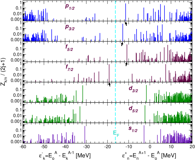
Figure 6: (Color online) Spectral strengths for one-neutron transfer on ⁵⁶Ni obtained from the self-consistent single-particle propagator $g(\omega)$. Poles above (below) the Fermi energy, $E_{F}$, correspond to transition to eigenstates of ⁵⁷Ni (⁵⁵Ni). The respective spectroscopic factors are given as a fraction of the independent-particle model value. The quasiparticle poles corresponding to the valence orbits of the $1p0f$ shell are indicated by arrows. A logarithmic scale was chosen to put in stronger evidence the distribution of the fragmented strength. Results are for $\hbar\Omega$=10 MeV, $N_{max}$=9 and $\kappa_{M}$=0.57 MeV.

The information carried by the calculated single-particle propagator $g(\omega)$ is collected in Fig. 6 for neutrons and partial waves up to $l$=3. The plot shows the spectral strength associated with each pole of $g(\omega)$. Fragments below the Fermi surface ($E_{F}$) refer to the separation of a neutron (⁵⁵Ni), while those above correspond to neutron addition (⁵⁷Ni). The poles corresponding to the $1p0f$ valence orbits are indicated by arrows. These are the same single-particle energies that have been discussed in Sec. III.2 and Tab. 1. As noted above, the fragments found at slightly higher energies (just above $\varepsilon^{+}_{n}\sim-8$ MeV) originate from the mixing of these orbits with two-particle-one-hole configurations and collective excitations of the nucleus. The overall fragmentation effect is substantial but not strong enough to destroy the single-particle character of the principal quasiparticle peaks (note that a logarithmic scale has been chosen in Fig. 6 in order to make smaller fragments of the spectral distribution more visible). This observation supports the use of valence single-particle states as the relevant degrees of freedom that govern low-lying excitations, as assumed in conventional shell-model applications. We note that the question whether a system can be approximated as a good shell closure is better addressed by analyzing the spectroscopic factors and strength distribution rather than occupation numbers, since the latter are integrated quantities . While unoccupied states can be probed by the addition of a nucleon, occupied states are accessed by knockout to states of the $A-1$ nucleon system. A similar fragmentation pattern is therefore seen for the $0f_{7/2}$ orbit but reversed below the Fermi surface. Interestingly enough, the Faddeev random phase approximation predicts that states corresponding to orbits in the $1s0d$ and $2s1d0g$ shells maintain a strong single-particle character even though they are further apart from the Fermi surface. The fragmentation of these orbits requires excitations across shells of different parity (e.g. $1s0d$ and $1p0f$) and could become stronger if the energy difference among major shells is reduced. Indeed, a comparison of our results with electron scattering measurements on ⁵⁸Ni Mou.76 suggests that the N³LO interaction tends to overestimate the gaps between these major shells. Note that in the present calculations the $2s1d0g$ quasiparticles are found at energies of about $-3$ MeV and overlap with the fragmented $1p0f$ states.

Far from the Fermi energy $E_{F}$, the mixing with complex configurations becomes strong and it is no longer possible to identify sharp quasiparticle and quasihole states. Still, the energy region occupied by the major shells can be identified clearly. The N³LO interaction places the states associated with the $1s0d$ shell between $-60$ and $-30$  MeV, while the $0p$-shell states appear below $-50$ MeV. Other hole fragments are observed around $-30$ MeV for the $1p_{1/2}$, $1p_{3/2}$ and $0f_{5/2}$ partial waves. These originate from particle states in the $1p0f$ shell that are partially occupied due to the smearing of the Fermi surface. Nucleon knockout from these orbits requires little energy transfer and leads to low-lying states in ⁵⁵Ni or ⁵⁵Cu. These states originate from the mixing of particle orbits with two-hole-one-particle configurations ($R^{(2h1p)}$) in the Dyson equation. Still, the ⁵⁵Ni ground state is strongly influenced by the $0f_{7/2}$ hole component.

Analogous fragmentation patterns extend to the shells further away from the Fermi surface, although these are not shown in Fig. 6. On the particle side, $\varepsilon^{+}_{n}=0$ MeV marks the threshold for the single-particle continuum in the $(A+1)$-nucleon system. Above this, the exact spectral function becomes a continuous function of energy. In the present calculations a structure of separate poles is found due to the discretization of the model space. A continuum distribution also develops for the hole part of the exact spectral function below the energy $\varepsilon^{-}_{k}$=$(E_{0}^{A}-E_{k^{\prime}=0}^{A-1})-S_{N}^{A-1}$, where $S_{N}^{A-1}$ is the one-nucleon separation energy from the ground state of $A-1$ particles. The distribution on both sides of the Fermi surface is similar but not fully symmetric, the strength being stronger at large positive energies. This is because the $(A+1)$-nucleon system can access a larger phase space than a single hole within the $A$-nucleon ground state. This asymmetry is already observed at the level of the self-energy $\Sigma^{\star}(\omega)$, a result in line with available fits of global optical potentials Cha.06 ; Cha.07 .

For the proton case, the poles of $g(\omega)$ correspond to the addition (removal) of a proton to the eigenstates of ⁵⁷Co (⁵⁵Cu). The corresponding spectral strength is substantially the same as that discussed for neutrons due to the almost exact isospin symmetry of the nuclear force. However, it is shifted to higher energies by the Coulomb repulsion.

V Conclusions

The aim of this work has been to extend large-scale calculations of self-consistent Green’s functions to medium mass nuclei and to investigate the properties of the single-particle spectral function of ⁵⁶Ni.

Many-body Green’s functions hold a number of interesting mathematical properties. Since one aims at obtaining excitations relative to a reference nucleus calculations scale more gently when increasing the number of particles as opposed to direct large-scale diagonalization methods. Only connected diagrams are summed to all orders so that the extensivity condition is satisfied bartlett2007 . Moreover, the self-consistent approach provides a path to ensure the conservation of basic macroscopic quantities. However, the greatest advantage of the self-consistent Green’s function formalism is that its building blocks, the many-body propagators, contain information on the response to several particle transfer and excitation processes. Therefore, they can be directly compared to a large body of experimental data. Due to these characteristics the formalism can be used to gain unmatched insights into the many-body dynamics of quantum mechanical systems. Within this framework, the Faddeev random phase approximation method proposed in Ref. Bar.01 is a good candidate to pursue ab initio studies of medium mass isotopes.

In this work we have presented the basic details of calculating the Faddeev random phase approximation expansion and discussed results for the spectral function of ⁵⁶Ni. This is the first application of the self-consistent Green’s function approach to the $1p0f$ shell region. The calculations employ the chiral N³LO two-nucleon interaction, with a modified monopole to account for missing many-nucleon forces. In addition to this one-parameter modification of the Hamiltonian, the only remaining parameters that enter our calculations are those defining the nucleon-nucleon interaction.

Calculations were performed in models spaces including up to ten major oscillator shells. These large spaces are large enough to allow for a sophisticated treatment of long-range correlations. The quasiparticle and quasihole energies of the $1p0f$ valence orbits were found to be rather well converged. In the largest calculations they appeared to be almost constant for oscillator frequencies in the range $\hbar\Omega\in[8,20]$ MeV. These convergence properties are possible thanks to a prediagonalization of the effects of short-range correlations. This is done using the $G$-matrix technique Hjo.95 ; CENS.08 to resum ladder diagrams outside the model space. Our results put in evidence the strong sensitivity of spectroscopic factors on the particle-hole gap at the Fermi surface. For the $N=28$ and $Z=28$ subshell closures the bare N³LO potential fails in describing the experimental gap (in an analogous way to other realistic two-nucleon interactions caurier2005 ). This effect has been attributed to missing three-nucleon interactions Zuk.03 . It is found that a proper correction of few monopole terms of the Hamiltonian allows us to extract reliable results for the fragmentation of single-particle strength.

Fully self-consistent Faddeev random phase approximation calculations have till now only been presented for ¹⁶O. The extension to accurate ab initio calculations in the $1p0f$ shell represent a major technical advance. However, no substantial use of parallel computation has been made in applying this formalism. Improvements in numerical algorithms are still possible and it is expected that they will allow a better treatment of fragmentation in the self-consistent approach, as well as pushing the limits of present calculations well beyond mass $A=56$. Another obvious extension is the inclusion of explicit three-nucleon forces. Within the framework of self-consistent Green’s function theory this has already been achieved for nuclear matter studies Soma2008 . Similar developments can be expected for finite nuclei as well.

For open shell systems with weakly bound states and/or resonances, one needs a single-particle basis which can handle continuum states, as done in Hag.07 . Normally, this leads to a much larger space and may require parallelization of our codes. On the other hand, the effective interaction among valence-space quasiparticles is already generated in the present calculations and can be used for standard shell-model calculations in one or two major shells. The issue of degenerate unperturbed states for open shells systems has also been addressed for Green’s functions theory in Ref. Slu.93 by using a Bogoliubov-type quasi-particle transformation. In a self-consistent treatment, one may improve on this approach by extending the Faddeev-RPA method to include explicit configuration mixing between the nucleons inside the open shell.

The $N=28$ and $Z=28$ subshell closure has also attracted recent experimental interest following the discussion of whether the low-lying states of ⁵⁷Cu are strongly fragmented due to a soft ⁵⁶Ni core, see for example Ref. ni56f . While no direct experimental information is available for the transition between these two isotopes, the spectroscopic factor for neutron knockout from ⁵⁷Ni has been measured in Ref. Yur.06 . The present calculations describe well the quenching of the experimental cross section. At the same time, we report predictions for both proton and neutron transfer to the other valence orbits around ⁵⁶Ni. These calculations can thereby provide theoretical benchmarks for the forthcoming experiments of Refs. ni56c ; ni56d . These spectroscopic factors are all in the range of 60%-70% of the independent-particle model value and in fair agreement with the observation of valence states in several stable nuclei lap93 . The fragmentation pattern of valence orbits predicted by the Faddeev random phase approximation is also found in substantial agreement with what is known for closed shell nuclei Dic.04 and supports the description of ⁵⁶Ni as a doubly magic nucleus. Finally, we note that the effects of admixing configurations with several particle-hole excitations are not included in the present study. These effects can be accounted for by using configuration interaction (shell-model) methods. However, based on the analysis of Refs. Hor.07 ; Gou.08 ; newpap these corrections are not expected to be dominant.

- (1) K. L. Yurkewicz et al, Phys. Rev. C 70, 064321 (2004).
- (2) K. L. Yurkewicz et al., Phys. Rev. C 74, 024304 (2006).
- (3) J. Lee, M. B. Tsang, W. G. Lynch, M. Horoi, and S. C. Su, preprint ArXiv:0809.4686; M. B. Tsang et al, preprint ArXiv:0810.1925 and National Superconducting Cyclotron Laboratory, Michigan State University, proposal 06035.
- (4) A. Gade et al, unpublished and National Superconducting Cyclotron Laboratory, Michigan State University, proposal 06020.
- (5) G. Kraus et al, Phys. Rev. Lett. 73, 1773 (1994).
- (6) K. Minamisono et al, Phys. Rev. Lett. 96, 102501 (2006).
- (7) D. Bazin et al, Phys. Rev. Lett. 101, 252501 (2008).
- (8) M. Horoi, B. A. Brown, T. Otsuka, M. Honma, and T. Mizusaki, Phys. Rev. C 73, 061305(R) (2006).
- (9) L. Lapikás, Nucl. Phys. A553, 297c (1993).
- (10) R. R. Whitehead, A. Watt, B. J. Cole, and I. Morrison, Adv. Nucl. Phys. 9, 123 (1977).
- (11) E. Caurier, G. Martinez-Pinedo, F. Nowacki, A. Poves, and A. P. Zuker, Rev. Mod. Phys. 77, 427 (2005).
- (12) D.J. Dean, T. Engeland, M. Hjorth-Jensen, M.P. Kartamyshev, and E. Osnes, Prog. Part. Nucl. Phys. 53, 419 (2004).
- (13) P. Navratil and E. Caurier, Phys. Rev. C 69, 014311 (2004).
- (14) R. J. Bartlett and M. Musial, Rev. Mod. Phys. 79, 291 (2007).
- (15) D. J. Dean and M. Hjorth-Jensen, Phys. Rev. C 69, 054320 (2004).
- (16) T. Helgaker, P. Jørgensen, and J. Olsen, Molecular Electronic Structure Theory. Energy and Wave Functions, (Wiley, Chichester, 2000).
- (17) G. Hagen, T. Papenbrock, D. J. Dean, and M. Hjorth-Jensen, Phys. Rev. Lett 101, 092502 (2008).
- (18) B. S. Pudliner, V. R. Pandharipande, J. Carlson, Steven C. Pieper, and R. B. Wiringa, Phys. Rev. C 56, 1720 (1997).
- (19) S.E. Koonin, D.J. Dean, and K. Langanke, Phys. Rep. 278, 1 (1997).
- (20) Y. Utsuno, T. Otsuka, T. Mizusaki, and M. Honma, Phys. Rev. C 60, 054315 (1999).
- (21) P. J. Ellis and E. Osnes, Rev. Mod. Phys. 49, 777 (1977).
- (22) M. Hjorth-Jensen, T. T. S. Kuo, and E. Osnes, Phys. Rep. 261, 125 (1995).
- (23) W. H. Dickhoff and D. Van Neck, Many-Body Theory Exposed! (World Scientific, Singapore, 2005).
- (24) W. H. Dickhoff and C. Barbieri, Prog. Part. Nucl. Phys. 52, 377 (2004).
- (25) Y. Dewulf, D. Van Neck, and M. Waroquier, Phys. Rev. C 65, 054316 (2002).
- (26) D. Van Neck, S. Rombouts, and S. Verdonck, Phys. Rev. C 72, 054318 (2005).
- (27) Y. Dewulf, W. H. Dickhoff, D. Van Neck, E. R. Stoddard, and M. Waroquier, Phys. Rev. Lett. 90, 152501 (2003).
- (28) C. Barbieri and W. H. Dickhoff, Phys. Rev. C 63, 034313 (2001).
- (29) C. Barbieri and W. H. Dickhoff, Phys. Rev. C 65, 064313 (2002).
- (30) C. Barbieri and W. H. Dickhoff, Phys. Rev. C 68, 014311 (2003).
- (31) C. Barbieri, Phys. Lett. B643, 268 (2006).
- (32) S. R. White, Phys. Rev. Lett. 69, 2863 (1992).
- (33) U. Schollwock, Rev. Mod. Phys. 77, 259 (2005).
- (34) J. Dukelsky, S. Pittel, S. S. Dimitrova, and M. V. Stoitsov, Phys. Rev. C 65, 054319 (2002).
- (35) B. Thakur, S. Pittel, and N. Sandulescu, Phys. Rev. C 78, 041303(R) (2008).
- (36) R. J. Bartlett, V. F. Lotrich, and I. V. Schweigert, J. Chem. Phys. 123, 062205, (2005).
- (37) D. Van Neck, S. Verdonck, G. Bonny, P. W. Ayers, and M. Waroquier, Phys. Rev. A 74, 042501 (2006).
- (38) Steven C. Pieper, V. R. Pandharipande, R. B. Wiringa, and J. Carlson, Phys. Rev. C 64, 014001 (2001).
- (39) R. B. Wiringa and Steven C. Pieper, Phys. Rev. Lett. 89, 182501 (2002).
- (40) S. C. Pieper, R. B. Wiringa, and J. Carlson, Phys. Rev. C 70, 054325 (2004).
- (41) P. Navrátil and B. R. Barrett, Phys. Rev. C 57, 562 (1998).
- (42) P. Navrátil, G. P. Kamuntavicius, and B. R. Barrett, Phys. Rev. C 61, 044001 (2000).
- (43) P. Navrátil and W. E. Ormand, Phys. Rev. Lett. 88, 152502 (2002).
- (44) P. Navrátil, J. P. Vary, and B. R. Barrett, Phys. Rev. C 62, 054311 (2000).
- (45) P. Navratil and W. E. Ormand, Phys. Rev. C 68, 034305 (2003).
- (46) A. Nogga, P. Navratil, B. R. Barrett, and J. P. Vary, Phys. Rev. C 73, 064002 (2006).
- (47) D. R. Entem and R. Machleidt, Phys. Rev. C 68, 041001(R) (2003).
- (48) G. Hagen, private communication (2009).
- (49) R. J. Charity, L. G. Sobotka, W. H. Dickhoff, Phys. Rev. Lett. 97, 162503 (2006).
- (50) R. J. Charity, J. M. Mueller, L. G. Sobotka, W. H. Dickhoff, Phys. Rev. C 76, 044314 (2007).
- (51) C. Barbieri, D. Van Neck, and W. H. Dickhoff, Phys. Rev. A 76, 052503 (2007).
- (52) C. Barbieri and W. H. Dickhoff, arXiv:0901.1920v1 [nucl-th], (2009).
- (53) C. Barbieri, C. Giusti, F. D. Pacati, W. H. Dickhoff, Phys. Rev. C70, 014606 (2004).
- (54) D. G. Middleton et. al., Eur. Phys. J. A29, 261 (2006).
- (55) C. Barbieri and B. K. Jennings, Phys. Rev. C72, 014613 (2005).
- (56) H. Müther, A. Polls, and W. H. Dickhoff, Phys. Rev. C 51, 3040 (1995).
- (57) W. J. W. Geurts, K. Allaart, W. H. Dickhoff, and H. Müther, Phys. Rev. C 53, 2207 (1996).
- (58) R. B. Wiringa, V. G. J. Stoks, and R. Schiavilla, Phys. Rev. C 51, 38 (1995).
- (59) A. L. Fetter and J. D. Walecka, Quantum Theory of Many-Particle Physics (McGraw-Hill, New York, 1971).
- (60) T. Engeland, M. Hjorth-Jensen, and G. R. Jansen, CENS, a Computational Environment for Nuclear Structure. The codes are freely available at the link http://www.fys.uio.no/compphys/software.html.
- (61) I. Stetcu, B. R. Barrett, P. Navrátil, and J. P. Vary, Phys. Rev. C 71, 044325 (2005).
- (62) Kh. Gad and H. Müther, Phys. Rev. C 66, 044301 (2002).
- (63) L. D. Faddeev, Zh. Éksp. Teor. Fiz. 39 1459 (1961) [Sov. Phys. JETP 12, 1014 (1961)].
- (64) G. Baym and L. P. Kadanoff, Phys. Rev. 124, 287 (1961).
- (65) G. Baym, Phys. Rev. 127, 1391 (1962).
- (66) G. Onida, L. Reining, and A. Rubio, Rev. Mod. Phys. 74, 601 (2001).
- (67) W. Arnoldi, Quart. Appl. Math. 9, 17 (1951).
- (68) M. Horoi, et al., Phys. Rev. Lett. 98, 112501 (2007).
- (69) A. P. Zuker, Phys. Rev. Lett. 90, 042502 (2003).
- (70) J. R. Gour, P. Piecuch, M. Hjorth-Jensen, M. Wloch, and D. J. Dean, Phys. Rev. C 74, 024310 (2006).
- (71) M. Wloch, D. J. Dean, J. R. Gour, M. Hjorth-Jensen, K. Kowalski, T. Papenbrock, and P. Piecuch, Phys. Rev. Lett. 94, 212501 (2005).
- (72) R. B. Firestone, V. S. Shirley, C. M. Baglin, S. Y. Frank Chu, and J. Zipkin, Table of Isotopes, 8th ed. (Wiley Interscience, New York, 1996).
- (73) C. R. Gould et al., Phys. Rev. C 188, 1792 (1969).
- (74) A. Gade et al., Phys. Rev. C 77, 044306 (2008).
- (75) J. Mougey, et al.,Nucl. Phys. A262, 461 (1976).
- (76) V. Somà and P. Bożek, Phys. Rev. C 78, 054003 (2008).
- (77) G. Hagen, D. J. Dean, M. Hjorth-Jensen, and T. Papenbrock, Phys. Lett. B656, 169 (2007).
- (78) V. Vav den Sluys, D. Van Neck, M. Waroquier, and J. Ryckebusch, Nucl. Phys. A551, 210 (1993).
- (79) J. R. Gour, M. Horoi, P. Piecuch, B. A. Brown, Phys. Rev. Lett. 101, 052501 (2008).
- (80) C. Barbieri, M. Hjorth-Jensen, in preparation.