Multiplicity Fluctuations and Correlations in
Limited Momentum Space Bins in Relativistic Gases

Abstract

Multiplicity fluctuations and correlations are calculated within thermalized relativistic ideal quantum gases. These are shown to be sensitive to the choice of statistical ensemble as well as to the choice of acceptance window in momentum space. It is furthermore shown that global conservation laws introduce non-trivial correlations between disconnected regions in momentum space, even in the absence of any dynamics.

I Introduction

Fluctuations of, and correlations between, various experimental observables are believed to have the potential to reveal new physics. The growing interest in event-by-event fluctuations in strong interactions is motivated by expected anomalies in the vicinity of the onset of deconfinement OnsetOfDecon ; koch1 ; asakawa ; koch2 and in the case when the expanding system goes through the transition line between quark-gluon plasma and hadron gas PhaseTrans . In particular, a critical point of strongly interacting matter may be accompanied by a characteristic power-law pattern in fluctuations CriticalPoint . Recently, it has been suggested that correlations across a large interval of rapidity arise from a color glass condensate correlation_cgc1 ; correlation_cgc2 . In recent years a wide range of experimental measurements of fluctuations of particle multiplicities fluc-mult ; BeniData , transverse momenta fluc-pT and multiplicity correlations in rapidity tarnowsky ; PHENIX_rap_corr ; PHOBOS_rap_corr have been reported, leading to a lively discussion regarding their physical interpretation GMC ; bzdak ; correlation_cgc2 ; tarnowsky .

To get a reliable indication of new physics, it is important to note that most fluctuation and correlation observables are also sensitive to some “baseline” contributions that, nevertheless, can have non-trivial behaviour. For instance, most fluctuation and correlation observables are sensitive to the global characteristics (e.g. the distribution of the number of colliding nucleons) of a sample of events, which can in turn be non-trivially constrained by centrality bin construction GMC . Similarly, conservation laws can provide a “trivial” correlation between observables. The effects of such correlations depend on the scale at which these conservation laws become important. This scale could be anything, from microscopic (mean free path, diffusion scale) to the macroscopic size of the system.

The purpose of this paper is to study these baseline correlations in a limiting case: that of a thermalized relativistic ideal (no inter-particle interactions) quantum gas for which we want to assess the importance of globally applied conservation laws for particle multiplicity fluctuations and correlations. In this case, all observables are calculable simply using statistical mechanics techniques. Such an approach has a long and distinguished history of calculating particle multiplicities in hadronic collisions  Fer50 ; Pom51 ; Lan53 ; Hag65 ; bdm ; equil_energy ; jansbook ; becattini ; nuxu ; share ; sharev2 ; thermus .

Conventionally in statistical mechanics three standard ensembles are discussed; the micro canonical ensemble (MCE), the canonical ensemble (CE), and the grand canonical ensemble (GCE). In the MCE one considers an ensemble of micro states with exactly fixed values of extensive conserved quantities (energy, momentum, electric charge, etc.), with ‘a priori equal probabilities‘ of all micro states (see e.g. Patriha ). The CE introduces the concept of temperature by introduction of an infinite thermal bath, which can exchange energy (and momentum) with the system. The GCE introduces further chemical potentials by attaching the system under consideration to an infinite charge bath. Only if the experimentally accessible system is only a small fraction of the total, and all parts have had the opportunity to mutually equilibrate, can the appropriate ensemble be the Grand Canonical one.

In the limit of very large volume and constant density (the thermodynamic limit), average values of intensive quantities are the same for all ensembles. However, even in this limit, these ensembles have different properties with respect to fluctuations and correlations SM_fluc_ce . In the MCE, energy and charge are exactly fixed. In the CE, charge remains fixed, while energy is allowed to fluctuate about some average value. Finally in the GCE the requirement of exact charge conservation is dropped, too. One may also consider isobaric ensembles isobar , or even more general ‘extended Gaussian ensembles‘ extgauss ; alpha . In previous articles SM_fluc_ce ; CE_Res ; MCEvsData ; SM_fluc_mce ; VdWFluc ; QstatsNearTL ; BoseCond ; clt ; acc ; isobar ; alpha it was shown that these differences mean that multiplicity fluctuations are ultimately ensemble specific.

In this article we extend these results to fluctuations and correlations between particle multiplicities in limited bins of momentum space (rapidity $y$, transverse momentum $p_{T}$ and azimuthal angle $\phi$). In section II we present details of the calculation of correlations within statistical mechanics. The following two sections present calculated fluctuations and correlations within the same momentum space bin for a stationary (section III.1) and boosted (section III.2) system. In section IV we discuss long range correlations between momentum space bins. A discussion section V, summarising our results and discussing their phenomenological implications within the context of heavy ion collisions, closes the paper.

II Correlations and Fluctuations within different Ensembles

In a recent paper clt we have shown that GCE joint distributions of extensive quantities converge to Multivariate Normal Distributions (MND) in the thermodynamic limit (TL). MCE or CE multiplicity distributions could then be defined through conditional GCE distributions. In general one may write for the multiplicity distribution $P_{ce}(N)$ of a CE with conserved electric charge $Q$:

$$P_{ce}(N)~{}=~{}\frac{\textrm{number of all states with $Q$ and $N$}}{\textrm{number of all states with $Q$ }}~{}.$$ (1)

Likewise one can write for the CE joint multiplicity distribution of particle species $A$ and $B$:

$$P_{ce}(N_{A},N_{B})~{}=~{}\frac{\textrm{number of all states with $Q$, $N_{A}$ and $N_{B}$}}{\textrm{number of all states with $Q$ }}~{}.$$ (2)

The number of all micro states with electric charge $Q$, and multiplicities $N_{A}$ and $N_{B}$ of a system with temperature $T$ and volume $V$ is given by the CE partition function $Z_{CE}(V,T,Q,N_{A},N_{B})$. Similarly, $Z_{CE}(V,T,Q)$ denotes the number of micro states with fixed electric charge $Q$, but arbitrary multiplicities $N_{A}$ and $N_{B}$, for the same physical system.

The strategy to calculate joint multiplicity distributions could thus be the following (in principle also valid at finite volume):

$$P_{ce}(N_{A},N_{B}) = \frac{Z_{CE}(V,T,Q,N_{A},N_{B})}{Z_{CE}(V,T,Q)}~{},$$ (3)

$$= \frac{e^{Q\frac{\mu}{T}}~{}Z_{CE}(V,T,Q,N_{A},N_{B})}{Z_{GCE}(V,T,\mu)}~{}\frac{Z_{GCE}(V,T,\mu)}{e^{Q\frac{\mu}{T}}~{}Z_{CE}(V,T,Q)}~{},$$ (4)

$$= P_{gce}(Q,N_{A},N_{B})~{}P_{gce}^{-1}(Q)~{}=~{}P_{gce}(N_{A},N_{B}|Q)~{}.$$ (5)

In order to get from Eq.(3) to Eq.(5) both canonical partition functions $Z_{CE}(V,T,Q,N_{A},N_{B})$ and $Z_{CE}(V,T,Q)$ are divided by their GCE counterpart $Z_{GCE}(V,T,\mu)$ and multiplied by $e^{Q\frac{\mu}{T}}$. The first term on the right hand side of Eq.(4) then equals the GCE joint distribution $P_{gce}(Q,N_{A},N_{B})$, while the second term is just the inverse of the GCE charge distribution $P_{gce}(Q)$. Their ratio is the (normalised) GCE conditional distribution of particle multiplicities $N_{A}$ and $N_{B}$ at fixed electric charge $Q$, $P_{gce}(N_{A},N_{B}|Q)$, and equals the CE distribution $P_{ce}(N_{A},N_{B})$ at the same value of $Q$. This result is independent of the choice of chemical potential $\mu$.

The problem of finding a solution, or a (large volume) approximation, to the CE distribution $P_{ce}(N_{A},N_{B})$ is now turned into the problem of finding a solution or approximation to the GCE distribution of multiplicities $N_{A}$ and $N_{B}$, and charge $Q$. The role of chemical potential (or Lagrange multiplier) $\mu$ will be discussed in Section III.

From the assumption that the GCE distribution $P_{gce}(Q,N_{A},N_{B})$ converges to a Tri-variate Normal Distribution, it also follows that the marginal distribution $P_{gce}(Q)$, as well as the conditional distribution $P_{gce}(N_{A},N_{B}|Q)$, are Normal Distributions. Hence, $P_{ce}(N_{A},N_{B})$ should have a good approximation in a Bivariate Normal Distribution (BND) in the large volume limit (where the large particle numbers can be appropriately treated as continuous):

$$P_{BND}(N_{A},N_{B}) = \frac{1}{2\pi V\sqrt{\sigma_{A}^{2}\sigma_{B}^{2}\left(1-\rho^{2}\right)}}$$

$$\times \exp\Bigg{[}-\frac{1}{2V}\Bigg{[}\frac{\left(\Delta N_{A}\right)^{2}}{\sigma_{A}^{2}\left(1-\rho^{2}\right)}-2\rho\frac{\left(\Delta N_{A}\right)\left(\Delta N_{B}\right)}{\sigma_{A}\sigma_{B}\left(1-\rho^{2}\right)}+\frac{\left(\Delta N_{B}\right)^{2}}{\sigma_{B}^{2}\left(1-\rho^{2}\right)}\Bigg{]}\Bigg{]}~{},$$

where $\Delta N_{X}=N_{X}-\langle N_{X}\rangle$, with $X=A,B$ and:

$$V\sigma_{A}^{2} \equiv \langle N_{A}^{2}\rangle~{}-~{}\langle N_{A}\rangle^{2}~{},$$ (7)

$$V\sigma_{B}^{2} \equiv \langle N_{B}^{2}\rangle~{}-~{}\langle N_{B}\rangle^{2}~{},$$ (8)

$$V\sigma_{AB} \equiv \langle N_{A}N_{B}\rangle~{}-~{}\langle N_{A}\rangle\langle N_{B}\rangle~{}.$$ (9)

Here $V\sigma_{A}^{2}$ and $V\sigma_{B}^{2}$ are the variances of the marginal multiplicity distributions of particles $N_{A}$ and $N_{B}$. The term $V\sigma_{AB}$ is called the co-variance. Additionally we define the scaled variance $\omega_{X}$:

$$\omega_{X}~{}=~{}\frac{\langle N_{X}^{2}\rangle~{}-~{}\langle N_{X}\rangle^{2}}{\langle N_{X}\rangle}~{},$$ (10)

which measures the width of the marginal distribution $P(N_{X})$. Lastly,

$$\rho~{}\equiv~{}\frac{\sigma_{AB}}{\sigma_{A}\sigma_{B}}~{},$$ (11)

is the correlation coefficient between particle numbers $N_{A}$ and $N_{B}$.

The distribution Eq.(II) hence has 5 parameters: Mean values $\langle N_{A}\rangle$ and $\langle N_{B}\rangle$, variances of marginal distributions $V\sigma_{A}^{2}$ and $V\sigma_{B}^{2}$, and the correlation coefficient $\rho$. Loosely speaking, the correlation coefficient $\rho$ defines how the BND, Eq.(II), is tilted. In the case where $\rho>0$, the distribution is elongated along the main diagonal, and measuring a larger (smaller) number of particles $N_{A}$ implies that it is also more likely to measure a larger (smaller) number of particles $N_{B}$. The distribution is tilted the other way, if $\rho<0$. In this case, multiplicities $N_{A}$ and $N_{B}$ are anti-correlated, and measuring $N_{A}>\langle N_{A}\rangle$ implies that it is now more likely to measure $N_{B}<\langle N_{B}\rangle$. Particle numbers $N_{A}$ and $N_{B}$ are uncorrelated, if $\rho=0$.

Similarly, we define MCE multiplicity distributions in terms of conditional GCE distributions of extensive quantities. For this we will first find a suitable approximation to the GCE joint distribution of extensive quantities (electric charge, energy, momentum, particle number(s), etc.) by Fourier analysis of the GCE partition function. The MCE multiplicity distribution is then given by a slice along a surface of constant values of extensive quantities.

II.1 GCE Partition Function

The GCE partition function of a relativistic gas with volume $V$, local temperature $T=1/\beta$, chemical potentials $\vec{\mu}$ and collective four velocity $\vec{u}$ reads (the system four-temperature fourtemp is $\vec{\beta}~{}=~{}\beta\vec{u}$):

$$Z_{GCE}(V,\beta,\vec{\mu},\vec{u})~{}=~{}\exp\Bigg{[}V\Psi\left(\beta,\vec{\mu},\vec{u}\right)\Bigg{]}~{},$$ (12)

where $\Psi\left(\beta,\vec{\mu},\vec{u}\right)$ is a sum over the single particle partition functions $\psi_{l}\left(\beta,\vec{\mu},\vec{u}\right)$ of all particle species ‘$l$‘ considered in the model:

$$\Psi\left(\beta,\vec{\mu},\vec{u}\right)~{}=~{}\sum_{l}~{}\psi_{l}\left(\beta,\vec{\mu},\vec{u}\right)~{}.$$ (13)

The single particle partition function $\psi_{l}\left(\beta,\vec{\mu},\vec{u}\right)$ of particle species ‘$l$‘ is given by a Jüttner distribution:

$$\psi_{l}\left(\beta,\vec{\mu},\vec{u}\right)~{}=~{}\frac{g_{l}}{\left(2\pi\right)^{3}}~{}\int d^{3}p~{}\ln\left(1~{}\pm~{}e^{-\beta~{}p_{l}^{\mu}~{}u_{\mu}~{}+~{}\beta~{}q_{l}^{j}~{}\mu_{j}}\right)^{\pm 1}~{},$$ (14)

where $p_{l}^{\mu}$ are the components of the four momentum, $q_{l}^{j}$ are the components of the charge vector and $g_{l}$ is the degeneracy factor. The upper sign refers to Fermi-Dirac statistics (FD), while the lower sign refers to Bose-Einstein statistics (BE). The case of Maxwell-Boltzmann (MB) statistics is analogous.

In the following we restrict ourselves to systems moving along the $z$-axis and use variables $y$, $p_{T}$ and $\phi$. For a boost in rapidity of $y_{0}$ one finds for the four-velocity $\vec{u}$, the four-momentum $\vec{p}_{l}$ and the integral measure $d^{3}p$, respectively:

$$\vec{u} = \left(\cosh y_{0},~{}0,~{}0,~{}\sinh y_{0}\right)~{},$$ (15)

$$\vec{p}_{l} = \left(\sqrt{m_{l}^{2}+p_{T}^{2}}\cosh y,~{}p_{T}\cos\phi,~{}p_{T}\sin\phi,~{}\sqrt{m_{l}^{2}+p_{T}^{2}}\sinh y\right)~{},$$ (16)

$$d^{3}p = p_{T}~{}\sqrt{m_{l}^{2}+p_{T}^{2}}~{}\cosh(y-y_{0})~{}dy~{}dp_{T}~{}d\phi~{},$$ (17)

where $m_{l}$ is the mass of a particle of species $l$. The single particle partition function Eq.(14) now reads:

$$\psi_{l}\left(\beta,\vec{\mu},\vec{u}\right)~{}=~{}\frac{g_{l}}{\left(2\pi\right)^{3}}\int\limits_{-\pi}^{\pi}d\phi\int\limits_{0}^{\infty}dp_{T}\int\limits_{-\infty}^{\infty}dy~{}p_{T}\sqrt{m_{l}^{2}+p_{T}^{2}}\cosh(y-y_{0})~{}\ln\left(1~{}\pm~{}e^{-\beta~{}p_{l}^{\mu}~{}u_{\mu}~{}+~{}\beta~{}q_{l}^{j}~{}\mu_{j}}\right)^{\pm 1}.$$ (18)

For the examples in the following sections we chose a simple gas with only one conserved charge, denoted as a ‘pion gas‘. The presented formulae are, however, also readily applicable to a hadron resonance gas (HRG). Depending on what system one may want to study, one introduces chemical potentials $\vec{\mu}$ and the ‘charge‘ vector $\vec{q}_{l}$ of particle species $l$:

$$\vec{\mu} = (\mu_{B},~{}\mu_{S},~{}\mu_{Q},~{}\mu_{N_{A}},~{}\mu_{N_{B}})\qquad\vec{q}_{l}=(b_{l},~{}s_{l},~{}q_{l},~{}n_{A}(\Omega),~{}n_{B}(\Omega))\qquad\textrm{for a HRG}~{},$$ (19)

$$\vec{\mu} = (\mu_{Q},~{}\mu_{N_{A}},~{}\mu_{N_{B}})\qquad\qquad\qquad\vec{q}_{l}=(q_{l},~{}n_{A}(\Omega),~{}n_{B}(\Omega))\qquad\qquad\textrm{for a pion gas}~{},$$ (20)

where $\mu_{B}$, $\mu_{S}$, and $\mu_{Q}$ are the baryon, strangeness, and electric charge chemical potentials, respectively. $\mu_{N_{A}}$ and $\mu_{N_{B}}$ are particle-specific chemical potentials, and could denote out of chemical equilibrium multiplicities of species ‘A‘ and ‘B‘, similar to phase space occupancy factors $\gamma_{S}$ gammaSfirst and $\gamma_{q}$ gammaQfirst . Throughout this paper we neglect finite density effects, so $\mu_{N_{A}}=\mu_{N_{B}}=0$.

In addition, $b_{l}$, $s_{l}$, and $q_{l}$ are the baryonic charge, the strangeness, and the electric charge of particle species ‘$l$‘. $\Omega$ is the momentum space bin in which we wish to measure particle multiplicity. $n_{A}(\Omega)=1$ if the momentum vector of the particle is within the acceptance, $n_{A}(\Omega)=0$ if not. The charge vector $\vec{q}_{l}$ also contains, to maintain a common notation for all particle species considered in Eq.(13), the ‘quantum‘ number $n_{B}(\Omega)$.

One may also be interested in correlations of, for instance, baryon number $B$ and strangeness $S$, as e.g. in Refs.QCD_Karsch ; Koch_hadronic_fluc . In this case, the $\Lambda$ particle, with $q_{\Lambda}=(1,-1,0,1,1)$, would be counted in groups $A$ and $B$, provided the momentum vector is within the acceptance $\Omega$.

II.2 Generating Function

To introduce the generating function of the charge distribution $Z_{GCE}(V,\beta,\vec{\mu},\vec{u};\vec{\phi},\vec{\alpha})$ in the GCE we substitute in Eq.(14):

$$\beta~{}\mu_{j} \rightarrow \beta~{}\mu_{j}~{}+~{}i\phi_{j}~{},$$ (21)

$$\beta~{}u_{\mu} \rightarrow \beta~{}u_{\mu}~{}-~{}i\alpha_{\mu}~{}.$$ (22)

The yet unnormalised joint probability distribution of extensive quantities $\vec{Q},\vec{P}$ in the GCE is then given by the Fourier transform of Eq.(12) after substitutions Eqs.(21,22):

$$\mathcal{Z}^{\vec{Q},\vec{P}}(V,\beta,\vec{\mu},\vec{u})~{}=~{}\int\limits_{-\pi}^{\pi}\frac{d^{J}\phi}{\left(2\pi\right)^{J}}~{}e^{-iQ^{j}\phi_{j}}~{}\int\limits_{-\infty}^{\infty}\frac{d^{4}\alpha}{\left(2\pi\right)^{4}}~{}e^{-iP^{\mu}\alpha_{\mu}}~{}\exp\Bigg{[}V\Psi\left(\beta,\vec{\mu},\vec{u};\vec{\phi},\vec{\alpha}\right)\Bigg{]}~{}.$$ (23)

More details of the calculation, in particular on the connection between the partition functions $\mathcal{Z}^{\vec{Q},\vec{P}}(V,\beta,\vec{\mu},\vec{u})$ and the conventional version $Z_{MCE}(V,\vec{Q},\vec{P})$ fourtemp ; fourtempII , can be found in Appendix A. Depending on the system under consideration, we introduce the vector of extensive quantities $\vec{Q}$ and corresponding Wick rotated fugacities $\vec{\phi}$:

$$\vec{Q} = (B,~{}S,~{}Q,N_{A},N_{B})\qquad\vec{\phi}=(\phi_{B},~{}\phi_{S},~{}\phi_{Q},~{}\phi_{N_{A}},~{}\phi_{N_{B}})\qquad\textrm{for a HRG}~{},$$ (24)

$$\vec{Q} = (Q,N_{A},N_{B})\qquad\qquad\quad\vec{\phi}=(\phi_{Q},~{}\phi_{N_{A}},~{}\phi_{N_{B}})\qquad\qquad\quad\textrm{for a pion gas}~{}.$$ (25)

Here $B$ is the baryon number, $S$ is the strangeness, and $Q$ is the electric charge of the system. Together with particle numbers $N_{A}$ and $N_{B}$ this would be a 5-dimensional distribution in the case of a CE HRG. Additionally for four-momentum conservation, yielding a 9-dimensional Fourier transform Eq.(23) for a MCE HRG, we write:

$$\vec{P}~{}=~{}(E,~{}P_{x},~{}P_{y},~{}P_{z})\qquad\vec{\alpha}~{}=~{}(\alpha_{E},~{}\alpha_{P_{x}},~{}\alpha_{P_{y}},~{}\alpha_{P_{z}})~{},$$ (26)

where $E$ is the energy and $P_{x}$, $P_{y}$, and $P_{z}$ are the components of the collective momentum of the system, while $\vec{\alpha}$ are the corresponding fugacities.

The integrand of Eq.(23) is sharply peaked at the origin $\vec{\phi}=\vec{\alpha}=\vec{0}$ in the TL clt . The main contribution therefore comes from a very small region. To see this, a second derivative test can be done on the integrand of Eq.(23) taking into account the first two terms of Eq.(29). The limits of integration can hence be extended to $\pm\infty$. The distinction between discrete (Kronecker $\delta$) and continuous quantities (Dirac $\delta$) is not relevant for the TL approximation, where particle number is a continuous variable to be integrated over. We thus proceed by Taylor expansion of Eq.(13). For this it is convenient to include everything into a common vector notation:

$$\vec{\mathcal{Q}}~{}=~{}\left(\vec{Q},~{}\vec{P}\right)\qquad\textrm{and}\qquad\vec{\theta}~{}=~{}\left(\vec{\phi},~{}\vec{\alpha}\right)~{}.$$ (27)

The dimensionality of the vector $\vec{\mathcal{Q}}$ is denoted as $J=2+3+4=9$ for a MCE HRG. We now expand the cumulant generating function, $\Psi\left(\beta,\vec{\mu},\vec{u};\vec{\theta}\right)$, in a Taylor series:

$$\Psi\left(\beta,\vec{\mu},\vec{u};\vec{\theta}\right)~{}\simeq~{}\sum\limits_{n=0}^{\infty}~{}\frac{i^{n}}{n!}~{}\kappa_{n}^{j_{1},j_{2},\dots,j_{n}}~{}\theta_{j_{1}}~{}\theta_{j_{2}}\dots\theta_{j_{n}}~{},$$ (28)

where the elements of the cumulant tensor, $\kappa_{n}^{j_{1},j_{2},\dots,j_{n}}$, are defined by:

$$\kappa_{n}^{j_{1},j_{2},\dots,j_{n}}~{}=\left(-i\right)^{n}~{}\frac{\partial^{n}\Psi}{\partial\theta_{j_{1}}\partial\theta_{j_{2}}\dots\partial\theta_{j_{n}}}\Bigg{|}_{\vec{\theta}=\vec{0}}~{}.$$ (29)

Generally cumulants are tensors of dimension $J$ and order $n$. The first cumulant is then a vector, while the second cumulant is a symmetric $J\times J$ matrix. A good approximation to Eq.(23) around the point $\vec{\mathcal{Q}}_{eq}=(\vec{Q}_{eq}$, $\vec{P}_{eq})$, can be found in terms of a Taylor expansion of Eq.(13) in $\vec{\theta}=(\vec{\phi},\vec{\alpha})$, if:

$$\frac{\partial\mathcal{Z}^{\vec{\mathcal{Q}}}(V,\beta,\vec{\mu},\vec{u})}{\partial\vec{\mathcal{Q}}}\Bigg{|}_{\vec{\mathcal{Q}}_{eq}}~{}=~{}0~{}.$$ (30)

Implicitly, Eq.(30) does not define chemical potentials $\vec{\mu}$ and four-temperature $\vec{\beta}=\beta\vec{u}$, but corresponding Lagrange multipliers which maximise the amplitude of the Fourier spectrum of the generating function for a desired value of $\vec{Q}_{eq}$ and $\vec{P}_{eq}$. Their values generally differ from the GCE set $(\beta,\vec{\mu},\vec{u})$, however they coincide in the TL. Lagrange multipliers can be used for finite volume corrections clt . In the following we restrict ourselves to the large volume approximation.

II.3 Joint Distributions

In the large volume limit, i.e. $V\rightarrow\infty$, one may use the asymptotic solution, and only consider the first two cumulants, Eq.(29). Substituting Eq.(28) into Eq.(23) yields a standard $J$ dimensional Gaussian integral with solution:

$$\mathcal{Z}^{\vec{\mathcal{Q}}}(V,T,\vec{\mu},\vec{u})~{}\simeq~{}Z_{GCE}(V,\beta,\vec{\mu},\vec{u})~{}\frac{1}{\left(2\pi V\right)^{J/2}}~{}\frac{1}{\det\sigma}~{}\exp\left[-\frac{1}{2}~{}\xi^{j}\xi_{j}\right]~{},$$ (31)

where the elements of the new variable $\vec{\xi}$ are defined by:

$$\xi^{j}~{}=~{}\left(\Delta\mathcal{Q}\right)^{k}~{}\left(\sigma^{-1}\right)_{k}^{j}~{}V^{-1/2}~{}.$$ (32)

The elements of the vector $(\Delta\vec{\mathcal{Q}})$ measure the distance of the charge vector $\vec{\mathcal{Q}}$ to the GCE mean $V\vec{\kappa}_{1}$:

$$\left(\Delta\mathcal{Q}\right)^{k}~{}\equiv~{}\left(\mathcal{Q}^{k}-V\kappa_{1}^{k}\right)~{},$$ (33)

and $\left(\sigma^{-1}\right)$ is the inverse square root of the second order cumulant $\kappa_{2}$:

$$\sigma^{-1}~{}\equiv~{}\kappa_{2}^{-1/2}~{}.$$ (34)

The GCE joint distribution of extensive quantities $\vec{\mathcal{Q}}$ is a MND:

$$P_{gce}(\vec{\mathcal{Q}})~{}=~{}\frac{\mathcal{Z}^{\vec{\mathcal{Q}}}(V,\beta,\vec{\mu},\vec{u})}{Z_{GCE}(V,\beta,\vec{\mu},\vec{u})}~{}\simeq~{}~{}\frac{1}{\left(2\pi V\right)^{J/2}}~{}\frac{1}{\det\sigma}~{}\exp\left[-\frac{1}{2}~{}\xi^{j}\xi_{j}\right]~{}.$$ (35)

Mean values in the TL are given by the first Taylor expansion terms, $\langle N_{A}\rangle=V\kappa_{1}^{N_{A}}$, $\langle Q\rangle=V\kappa_{1}^{Q}$, $\langle E\rangle=V\kappa_{1}^{E}$, etc. and converge to GCE values. To obtain a joint (two-dimensional) particle multiplicity distribution one has to take a two-dimensional slice of the ($J$ dimensional) GCE distribution, Eq.(35), around the peak of the extensive quantities which one is considering fixed. The co-variance tensor $\kappa_{2}$ will be spelled out explicitly and discussed in Section III.2. Further details of the calculation can be found in Appendix B.

III Fluctuations and Correlations within a Momentum Bin

III.1 Static System

Let us start by discussing properties of a static thermal system. We want to measure joint distributions of multiplicities $N_{A}$ and $N_{B}$ in limited bins of momentum space (of width $\Delta p_{T}$ for transverse momentum bins and $\Delta y$ for rapidity bins). Depending on the size and positions of the bins, one finds different fluctuations and correlations. Results will, in particular, be compared to the acceptance scaling approximation employed in MCEvsData ; CE_Res ; SM_fluc_ce , which assumes random observation of particles with a certain probability $q$, regardless of particle momentum (see also Appendix C). Corresponding results for scaled variance in MB statistics can also be found in acc .

For our examples we chose a gas with three degenerate massive particles (with positive, negative and zero charge) with mass ${m=0.140}$GeV in three different statistics (MB, FD, BE). The momentum spectra are assumed to be ideal GCE spectra, due to the large volume approximation. In Fig.(1) transverse momentum and rapidity spectra are shown for MB statistics. BE and FD statistics yield similar spectra, unless chemical potentials are large.

We can then define bins by requiring each bin to hold the same fraction of the total multiplicity. Note that in this case the width and position of bins $\Delta p_{T}$ and $\Delta y$ will strongly depend on the underlying momentum spectra. Our examples, in particular the FD case, are a little academic in the sense that there is no fermion of this mass. In a HRG, often applied to heavy ion collisions, the lightest fermion is the nucleon for which quantum effects are probably negligible.

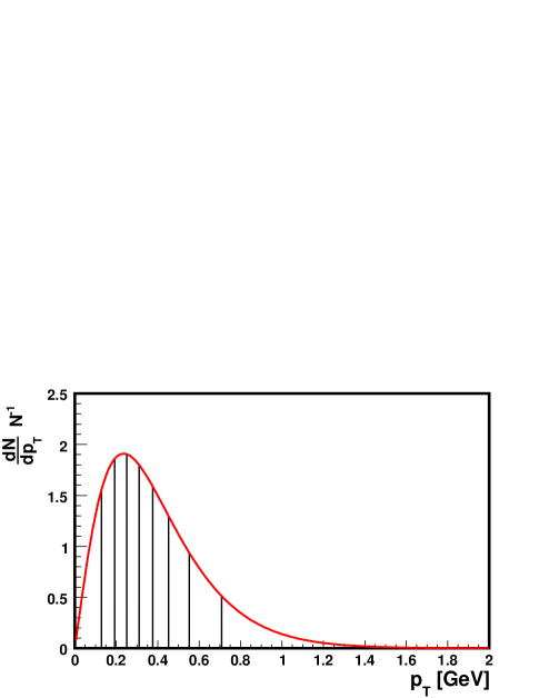
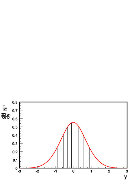
Figure 1: (Color online) Differential particle spectra for a ‘pion gas’ at $T=160$MeV. Transverse momentum spectrum (left) and rapidity spectrum (right). Both curves are normalised to unity. The bins are constructed such that each bin contains $1/9$ of the total yield.

In Fig.(2) we present the scaled variance $\omega$, calculated using Eq.(10), within different transverse momentum bins $\Delta p_{T}$ (left) and rapidity bins $\Delta y$ (right). The scaled variance in limited bins of momentum space is more sensitive to the choice of particle statistics than the spectra would suggest. BE and FD effects are particularly strong in momentum space bins in which occupation numbers are large. Hence, at the low momentum tail one finds suppression of fluctuations for FD and enhancement for BE, while at the high momentum tail, one finds $\omega_{BE}\simeq\omega_{MB}\simeq\omega_{FD}$, Fig.(2) (left). The rapidity dependence, Fig.(2) (right), has a different behaviour. The reason is, that in any $\Delta y$ bin there is some contribution from a low $p_{T}$ tail of the differential momentum spectrum $dN/dy/dp_{T}$ where quantum statistics effects are pronounced. This leads to a clear separation of the curves and one finds $\omega_{BE}~{}>~{}\omega_{MB}~{}>~{}\omega_{FD}$. In contrast to this, the $4\pi$ integrated (all particles observed) scaled variance is rather insensitive to the choice of statistics QstatsNearTL (unless chemical potentials are large). Please note that there are in fact 3 different ‘acceptance scaling‘ lines in Fig.(2), which extrapolate the $4\pi$ integrated scaled variance to limited acceptance. The differences are however very small and all 3 lines lie practically on top of each other.

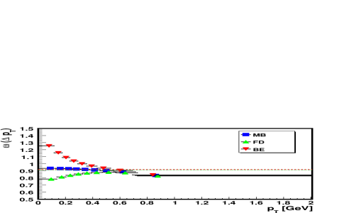
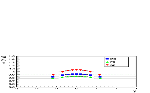
Figure 2: (Color online) Transverse momentum (left) and rapidity dependence (right) of the MCE scaled variance of negatively charged particles at $T=160$MeV, for a MB (blue), FD (green), BE (red) ‘pion gas’ at zero charge density. Momentum bins are constructed such that each bin contains the same fraction $q$ of the average $\pi^{-}$ yield. The horizontal bars indicate the width of the $\Delta p_{T}$ or $\Delta y$ bins, while the marker indicates the position of the center of gravity of the corresponding bin. Dashed lines indicate acceptance scaling results, Eq.(68).

In Fig.(3) we present the correlation coefficient $\rho$, calculated using Eq.(11), between positively and negatively charged particles in transverse momentum bins $\Delta p_{T}$ (left) and rapidity bins $\Delta y$ (right). The $4\pi$ integrated correlation coefficient between positively and negatively charged particles would be $\rho_{4\pi}=1$ in the CE and MCE. In the GCE it would be $0$. In the MB CE it would not show any momentum space dependence and would always be $\rho>0$. In the MCE the situation is qualitatively different: in low momentum bins particles are positively correlated, while in high momentum bins they can even be anti-correlated. Horizontal lines again indicate acceptance scaling (Appendix C). Quantum effects for the correlation coefficient remain small as there is no explicit local (quantum) correlations between particles of different charge.

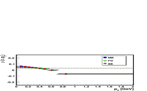
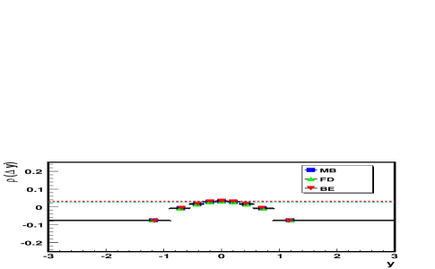
Figure 3: (Color online) Same as Fig.(2), but for the MCE correlation coefficient between positively and negatively charged particles. Dashed lines indicate acceptance scaling results, Eq.(71).

It should be stressed that the $\Delta p_{T}$ dependence in Figs.(2,3) is a direct consequence of energy conservation. The $\Delta y$ dependence of $\omega$ and $\rho$, however, is due to joint energy and longitudinal momentum ($P_{z}$) conservation. Disregarding $P_{z}$ conservation leads to a substantially milder $\Delta y$ dependence, see Fig.(4).

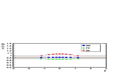
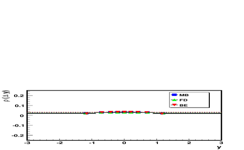
Figure 4: (Color online) Rapidity dependence of the scaled variance of positively charged particles (left) and of the correlation coefficient between positively and negatively charged particles (right). Calculations are done for the same system as in Figs.(2,3), however disregarding momentum conservation.

This behaviour can be intuitively explained: in a low momentum bin it is comparatively easy to balance charge, as each individual particle carries little energy and momentum. In contrast to this, in a high momentum bin with, say an excess of positively charged particles, it is unfavourable to balance charge, as one would also have to have more than on average negatively charged particles, and each particle carries large energy and momentum. This leads to suppressed fluctuations and correlations in high momentum bins when compared to low momentum bins.

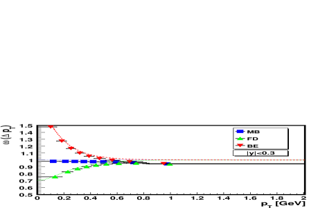
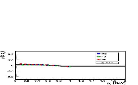
Figure 5: (Color online) Transverse momentum dependence of MCE scaled variance of negatively charged particles (left) and the MCE correlation coefficient between positively and negatively charged particles (right). Only particles in a mid-rapidity window $|y|<0.3$ are measured. Dashed lines denote the GCE result, Eq.(36).

In a small mid-rapidity window, with $|y|<0.3$, the effects of globally applied motional conservation laws cease to be important (see Fig.(5)). Local correlations due to BE and FD statistics begin to dominate, and MCE deviations from the GCE results, Eq.(36), are relevant only for the highest momentum bins. In BE or FD statistics we find for vanishing bin size ($\delta y,~{}\delta p_{T}$):

$$\omega^{GCE}_{\delta}~{}=~{}\frac{\kappa_{2}^{N_{\delta},N_{\delta}}}{\kappa_{1}^{N_{\delta}}}~{}\simeq~{}\frac{1}{1\pm e^{-\beta m_{T}\cosh y+\beta\mu}}~{}.$$ (36)

BE and FD effects are strongest around mid-rapidity $y=0$. MCE calculations in Fig.(5) are close to the GCE estimate Eq.(36). In MB statistics we find only a weak $\Delta p_{T}$ dependence in a small mid-rapidity window. Please note that the acceptance scaling procedure predicts a Poisson distribution with $\omega\rightarrow 1$ and $\rho\rightarrow 0$ for all three statistics in the limit of very small acceptance.

III.2 Collectively Moving System

As established a long time ago, in order to properly define the thermodynamics of a system with collective motion, the partition function needs to be Lorentz invariant Pathria_paper ; Touschek . The expectation values of observables need hence to transform according to the Lorentz transformation properties of these observables. In particular, the temperature $T$ is promoted to a four-vector $\beta^{\mu}$ (combining local temperature with collective velocity). The entropy, as well as particle multiplicities, remain Lorentz-scalars.

These requirements are in general not satisfied unless momentum conservation is put on an equal status with energy conservation. If the system is described by a MCE, then momentum should be conserved as well as energy Pathria_paper ; Touschek . If the system is exchanging energy with a bath, the bath needs to exchange momentum as well.

For ensemble averages, neglecting these rules and treating momentum differently from energy is safe as long as the system is close to the thermodynamic limit, since there ensembles become equivalent. The same is not true for fluctuation and correlation observables, which remain ensemble-specific SM_fluc_ce .

For a system at rest, these requirements are not apparent since the net momentum is zero. Statistical mechanics observables in a collectively moving system, however, lose their Lorentz invariance, if this is not maintained in the definition of the partition function.

To illustrate this point, we consider the properties of a system moving along the $z$-axis with a collective velocity given by Eq.(15). The total energy of the fireball is then $E=M\cosh(y_{0})$, while its total momentum is given by $P_{z}=M\sinh(y_{0})$. The mass of the fireball in its rest frame is $M=P^{\mu}u_{\mu}$. The system 4-temperature is $\vec{\beta}=\beta\vec{u}$. Local temperature and chemical potentials remain unchanged. We will use this section for a discussion of the second rank tensor (or co-variance matrix) $\kappa_{2}$, Eq.(29).

The second order cumulant $\kappa_{2}$, Eq.(29), is given by the second derivatives of the cumulant generating function with respect to the fugacities. Essentially this is the Hessian matrix hessian of the function Eq.(13), encoding the structure of its minima. The diagonal elements $\kappa_{2}^{X,X}$ are the variances of the GCE distributions of extensive quantities $X$. For example, $\kappa_{2}^{N_{A},N_{A}}$ measures the GCE variance of the distribution of particle multiplicity of species $A$, while $\kappa_{2}^{Q,Q}$ denotes the GCE electric charge fluctuations, etc. The off-diagonal $\kappa_{2}^{X,Y}$ elements give GCE co-variances of two extensive quantities $X$ and $Y$.

For a boost along the $z$-axis the general co-variance matrix for a pion gas reads:

$$\kappa_{2}=\begin{pmatrix}\kappa_{2}^{N_{A},N_{A}}&\kappa_{2}^{N_{A},N_{B}}&\kappa_{2}^{N_{A},Q}&\kappa_{2}^{N_{A},E}&\kappa_{2}^{N_{A},P_{x}}&\kappa_{2}^{N_{A},P_{y}}&\kappa_{2}^{N_{A},P_{z}}\\ \kappa_{2}^{N_{B},N_{A}}&\kappa_{2}^{N_{B},N_{B}}&\kappa_{2}^{N_{B},Q}&\kappa_{2}^{N_{B},E}&\kappa_{2}^{N_{B},P_{x}}&\kappa_{2}^{N_{B},P_{y}}&\kappa_{2}^{N_{B},P_{z}}\\ \kappa_{2}^{Q,N_{A}}&\kappa_{2}^{Q,N_{B}}&\kappa_{2}^{Q,Q}&\kappa_{2}^{Q,E}&0&0&0\\ \kappa_{2}^{E,N_{A}}&\kappa_{2}^{E,N_{B}}&\kappa_{2}^{E,Q}&\kappa_{2}^{E,E}&0&0&\kappa_{2}^{E,P_{z}}\\ \kappa_{2}^{P_{x},N_{A}}&\kappa_{2}^{P_{x},N_{B}}&0&0&\kappa_{2}^{P_{x},P_{x}}&0&0\\ \kappa_{2}^{P_{y},N_{A}}&\kappa_{2}^{P_{y},N_{B}}&0&0&0&\kappa_{2}^{P_{y},P_{y}}&0\\ \kappa_{2}^{P_{z},N_{A}}&\kappa_{2}^{P_{z},N_{B}}&0&\kappa_{2}^{P_{z},E}&0&0&\kappa_{2}^{P_{z},P_{z}}\end{pmatrix}~{}.$$ (37)

Off-diagonal elements correlating a globally conserved charge with one of the momenta, i.e. $\kappa_{2}^{Q,P_{x}}$, as well as elements denoting correlations between different momenta, i.e. $\kappa_{2}^{P_{x},P_{y}}$, are equal to zero due to antisymmetric momentum integrals. The values of elements correlating particle multiplicity and momenta, i.e. $\kappa_{2}^{N_{A},P_{x}}$, depend strongly on the acceptance cuts applied. For fully phase space integrated ($4\pi$) multiplicity fluctuations and correlations these elements are equal to $0$, again due to antisymmetric momentum integrals.

It is instructive to review the transformation properties of $\kappa$ under the Lorentz group: $\kappa_{2}^{X,Y}$ contains the correlations between 4-momenta $P^{\mu}$ and, in general, (scalar) conserved quantities and particle multiplicities $Q^{j}$. Hence, the elements $\kappa_{2}^{P^{\mu},P^{\nu}}$, i.e. $\left\langle\Delta P^{\mu}\Delta P^{\nu}\right\rangle$, will transform as a tensor of rank 2 under Lorentz transformations; $\kappa_{2}^{P^{\mu},Q^{j}}$, i.e. $\left\langle\Delta P^{\mu}\Delta Q^{j}\right\rangle$, will transform as a vector (the rapidity distribution will simply shift); and the remaining $\kappa_{2}^{Q^{j},Q^{k}}$ will be scalars.

For a static system one finds for the co-variances $\kappa_{2}^{E,P_{x}}=\kappa_{2}^{E,P_{y}}=\kappa_{2}^{E,P_{z}}=0$. Under these two conditions, a static system and full particle acceptance, the eigenvalues of the matrix Eq.(37) factorise, and momentum conservation can be shown to drop out of the calculation acc .

For a boost along the $z$-axis (and arbitrary particle acceptance) it is the appearance of non-vanishing elements $\kappa_{2}^{P_{z},E}=\kappa_{2}^{E,P_{z}}\not=0$ which make the determinant of the matrix $\kappa_{2}$, Eq.(37), invariant against such a boost. Please note that still $\kappa_{2}^{P_{x},E}=\kappa_{2}^{P_{y},E}=0$.

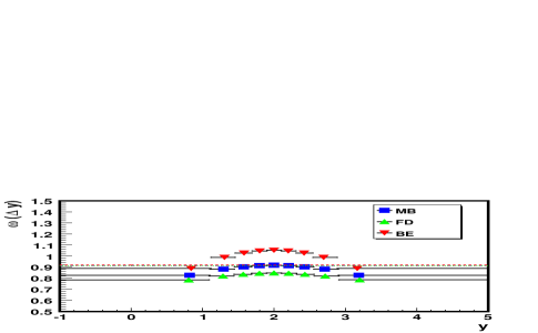
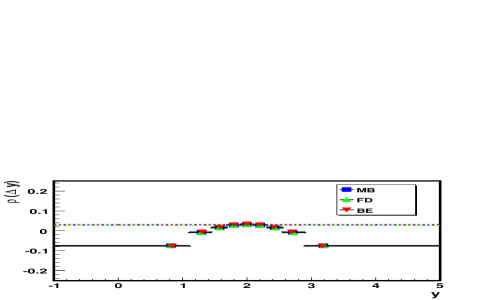
Figure 6: (Color online) Same as Fig.(2) (right) and Fig.(3) (right), but for a system moving with $y_{0}=2$.

In Fig.(6) we show multiplicity fluctuations (left) and correlations (right) for a system with boost $y_{0}=2$. The rapidity spectrum of Fig.(1) (right) is simply shifted to the right by two units. The construction of the acceptance bins is done as before. Multiplicity fluctuations and correlations within a bin transform as a vector (i.e., its $z$ component shifts in rapidity) as inferred from their Lorentz-transformation properties, provided both energy and momentum along the boost direction are conserved.

This last point deserves attention because usually (starting from Fer50 ) micro canonical calculations only conserve energy and not momentum. Imposing exact conservation for energy, and only average conservation of momentum will make the system non-Lorentz invariant, since in a different frame from the co-moving one energy and momentum will mix, resulting in micro state-by-micro state fluctuations in both momentum and energy.

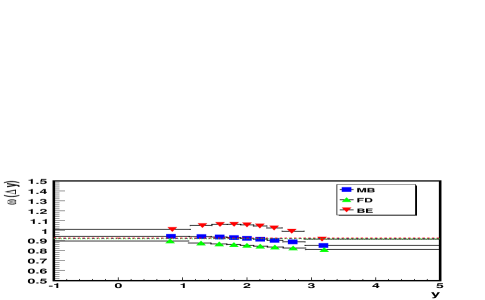
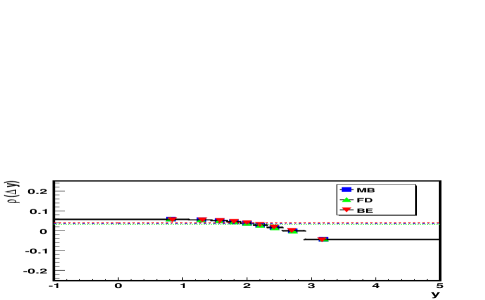
Figure 7: (Color online) Same as Fig.(6), but without $P_{z}$ exact conservation.

This situation is explicitly shown in Fig.(7). Here, we have calculated multiplicity fluctuations and correlations in the same system as in Fig.(6), but with exact conservation of only energy (and charge). In the co-moving frame of the system, the fluctuations and correlations are identical to Fig.(4). When the system is boosted, however, the distribution changes (not only by a shift in rapidity, as required by Lorentz-invariance), and loses its symmetry around the system’s average boost.

This last effect can be understood from the fact that momentum does not have to be conserved event by event, but energy does. It is easier, therefore, to create a particle with less rapidity than average (having less momentum than the boost, and parametrically less energy) than with more rapidity than average (having more momentum than the boost, and parametrically more energy) and still conserve energy overall. This leads to suppressed multiplicity fluctuations and a negative correlation coefficient for rapidity bins in the forward direction in comparison to rapidity bins in the backward direction. In Fig.(6), where the system also needs to conserve momentum exactly, this enhancement is balanced by the fact that it will be more difficult to conserve momentum when particles having less momentum than the boost are created.

A situation such as that in Fig.(7) is impossible to be realized physically. It could, however, be realized within “system in a box”-type calculations with non-equilibrium models: E.g., a transport model inside an infinitely heavy box (that absorbs momentum but not energy event-by-event) would end up exhibiting micro canonical correlations similar to those in Fig.(7). A similar box with ‘periodic‘ walls, however, would conserve energy as well as momentum inside the box, and should therefore behave as in Fig.(6). Thus, correlations within boosted sources provide a sensitive test of the Lorentz-invariance of such transport models.

IV Correlations between Bins disconnected in Momentum Space

“Long range correlations” between bins well disconnected in momentum have been suggested to arise from dynamical processes. Examples include color glass condensate correlation_cgc1 ; correlation_cgc2 , droplet formation driven hadronization ourbulk1 , and phase transitions within a percolation-type mechanism phasetrans_lrc ; cp_lrc . The elliptic flow measurements, widely believed to signify the production of a liquid at RHIC whitebrahms ; whitephobos ; whitestar ; whitephenix , are also, ultimately, correlations between particles disconnected in phase space (here, the azimuthal angle).

As we will show, however, conservation laws will also introduce such correlations between any two (connected or not) distinct regions of momentum space. No dynamical effects are taken into consideration (only an isotropic thermal system).

Let us first consider correlations between the multiplicities of particles $A$ and $B$, within two bins centered around $y_{A}$ and $y_{B}$, with (constant) widths $\Delta y_{A}=\Delta y_{B}=0.2$. In Fig.(8) (left) we show the correlation coefficient, calculated using Eq.(11), between positive and negative particles as a function of $y_{A}$ and $y_{B}$. In Fig.(8) (right) we show the correlation coefficient between like-charge, unlike-charge, and all charged particles as a function of $y_{gap}=y_{A}-y_{B}.$

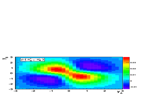
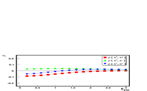
Figure 8: (Color online) Left: The correlation coefficient $\rho$ between the multiplicity of positively charged particles in a bin located at $y_{A}$ with negatively charged particles in a bin located at $y_{B}$, both with a 0.2 width in rapidity. Right: The correlation coefficient between multiplicities in two bins separated by $y_{gap}$ of like, unlike, and all charged particles. Both plots show MCE MB results.

Energy conservation always leads to anti-correlation between different momentum space bins. Charge conservation leads to a positive correlation of unlike charged particles and anti-correlation of like-sign particles. Longitudinal momentum conservation, however, is responsible for the structure visible in Fig.(8)(left). Having a small (large) number of particles in a bin with positive average longitudinal momentum, leads to a larger (smaller) number of particles in a bin with different but also positive $P_{z}$, (blue dips). This makes also a state with smaller (larger) particle number with opposite average longitudinal momentum $-P_{z}$ more likely (red hills). At large values of $y_{A}$ the correlation coefficient $\rho\simeq 0$ for any $y_{B}$, because the yield $\langle N_{A}\rangle$ in $\Delta y_{A}$ is asymptotically vanishing.

In Fig.(8) (right) we show the correlation coefficient along the diagonal from top left to bottom right as a function of separation. Unlike-sign particles are positively correlated. Like-sign and all charged particles are negatively correlated at small separation $y_{gap}$. For large separation the correlation becomes asymptotically zero, because the yield is zero. However, please note that in particular $\rho(\pi^{\pm},\pi^{\pm})>\rho(\pi^{+},\pi^{-})$ at large $y_{gap}$. $P_{z}$ conservation is dominant.

Disregarding $P_{z}$ conservation would destroy the particular structure in Fig.(8) (left) and lead to a single peak at the origin. The correlation would then be insensitive to the momentum direction, and only be sensitive to the energy content of a bin $\Delta y$. The observables in Fig.(8) transform under boosts ($y_{A,B}\rightarrow y_{A,B}-y_{0}$), provided momentum along the boost axis is exactly conserved.

Angular correlations also arise due to conservation of transverse momenta $P_{x}$ and $P_{y}$. In Fig.(9) we show the correlation coefficient between particles in different $\Delta\phi$ bins. The flat angular spectrum $dN/d\phi$ has been divided into 10 equal size bins and the correlation coefficient is presented as a function of separation of the centers of the corresponding bins.

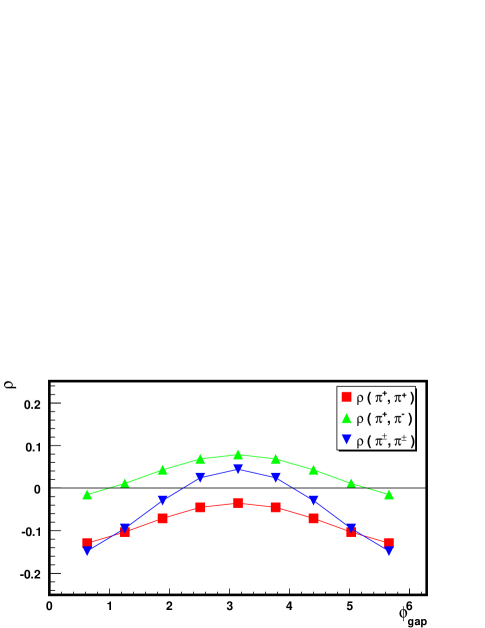
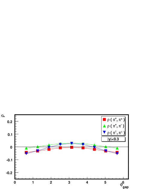
Figure 9: (Color online) The correlation coefficients of particles in distinct $\Delta\phi$ bins as a function of separation $\phi_{gap}$ in azimuth. (left) integrated over all phase space. (right) only particles with $|y|<0.3$ are observed. Both plots show MCE MB results. No elliptic flow is considered.

To explain Fig.(9) we note firstly that when disregarding exact conservation of $P_{x}$ and $P_{y}$ the correlation coefficients are insensitive to the distance $\phi_{gap}$ of any two bins. Only the correlations due to energy and charge conservation affect the result. Charge conservation leads to correlation of unlike-sign particles and to anti-correlation of like-sign particles. Energy conservation always anti-correlates multiplicities in two bins. For $\rho\left(\pi^{\pm},\pi^{\pm}\right)$ the effect of charge conservation cancels for a neutral system, however, effects of energy-momentum conservation are stronger, as a larger number of particles (hence a larger part of the total system) is observed.

Conservation of transverse momenta $P_{x}$ and $P_{y}$ is now responsible for the $\phi_{gap}$ dependence of $\rho$. The line of arguments is similar to the ones before: Observing a larger (smaller) number of particles in some bin at $\phi_{0}$ implies that, in order to balance momenta $P_{x}=P_{y}=0$, one should also observe a larger (smaller) number of particles in the opposite direction $\pi-\phi_{0}$. A larger (smaller) number of particles in a bin with $\phi_{gap}=\pi/2$ would do little to help to balance momentum, but conflict with energy conservation.

V Discussion and Summary

We have presented multiplicity fluctuations and correlations in limited momentum bins for ideal relativistic gases in the MCE in the thermodynamic limit. For our examples we chose a gas with three degenerate massive particles (positive, negative, neutral) in three different statistics (Maxwell-Boltzmann, Fermi-Dirac, Bose-Einstein).

For the width of multiplicity distributions in limited bins of momentum space a simple and intuitive picture emerges. In the Maxwell-Boltzmann approximation one finds a wider distribution for momentum bins with low average momentum when compared to bins with higher average momentum, but same average particle number. This qualitative behaviour is a direct consequence of energy and momentum conservation. The results in Fermi-Dirac and Bose-Einstein statistics, furthermore, show pronounced effects at the low momentum tail of the spectrum.

The correlation coefficient additionally shows a similar qualitative behaviour. In bins with low average momentum the correlation coefficient between positively and negatively charged particles is indeed positive, as one would expect from charge conservation. However, in bins with large average momentum the effects of joint energy and momentum conservation can lead to anti-correlated distributions of unlike-charged particles.

For boosted systems we found that the role of exactly imposed motional conservation laws is particularly important. Fluctuations and correlations transform under boosts, provided momentum conservation along the boost direction is taken into account. This ensures, in particular, that they become boost invariant if the underlying system is boost-invariant.

Lastly, we found that even in the thermodynamic limit long range correlations between disconnected regions in momentum space prevail. Multiplicities in different rapidity bins, as well as different bins in azimuth, have a non-zero correlation coefficient.

It is premature to use the model presented here for a quantitative comparison with experimental data. Firstly, the inclusion of resonances will provide important corrections. These can be implemented within our model using Monte-Carlo techniques, and will be the subject of a subsequent work mc .

An additional effect missing here that could change results qualitatively is longitudinal flow. It can be seen, “by symmetry”, that correlations and fluctuations in a perfectly boost-invariant fluid would be, just like other physical observables, independent of rapidity. Reconciling this with the calculations in sections III.1 and III.2 would require calculating correlations of many independent sources, each centered around a particular rapidity.

It is however not currently clear whether experimental data, even at highest RHIC and LHC energies at mid-rapidity, approximates this limit. At lower SPS energies, measurements  BeniData of the rapidity and transverse momentum dependence of particle multiplicity fluctuations show qualitatively similar results to those of our calculations (it should be noted that, as shown in benchmark , this behaviour for fluctuations also arises in molecular dynamics models, where conservation laws are included but equilibrium is not assumed). It has long been noticed busza ; busza2 that many observables binned in rapidity obey “universal fragmentation”, suggesting that a “Landau hydrodynamics”, with negligible initial longitudinal flow even away from mid-rapidity, might be more appropriate than boost-invariance to describe the initial state, even at ultra-relativistic energies steinberg . Experimentally, these measurements might be non-trivial since the size of the bins must be large enough for conservation laws to have an effect, but, since RHIC has large-acceptance data whitephobos ; whitebrahms and the LHC is planning a larger-acceptance detector totem , they are in principle possible.

If boost-invariance is not really there, then correlations and fluctuations binned by rapidity should be qualitatively similar to those calculated in section III.1 even at RHIC and LHC energies. We therefore suggest the experimental measurement of such fluctuations (Figs.(2,3) (right)) at these energies as an experimental probe of the degree of boost-invariance of the system.

Similarly, transverse flow should not change the correlation and fluctuations within limited transverse momentum bins (the left panels of Figs.(2,3)) beyond a trivial shift provided there are no significant fluctuations in collective flow observables. These fluctuations are widely expected to arise in an imperfect fluid vogel , but have remarkably not been observed, for example, in elliptic flow measurements loizides ; sorensen . We suggest, therefore, that a measurement of $p_{T}$ binned fluctuations and correlations could provide a qualitative way to assess the magnitude of event-by-event flow observables wrt to the thermal observables presented here.

Finally, effects of the sort studied in section IV will surely appear in any measurement looking for correlations across momentum space. Long range rapidity correlations have, in particular, been advocated as a signature of new physics correlation_cgc1 ; correlation_cgc2 . Our work shows that correlations due to conservation laws actually cover as wide a range in rapidity as those measured in tarnowsky ; PHENIX_rap_corr ; PHOBOS_rap_corr . The magnitude of the correlations, however, is significantly (as much as an order of magnitude) lower than either the experimental result or any reasonable “new physics”, suggesting that the origin of the experimentally observed correlations lies elsewhere. In particular, correlations induced by initial state geometry are considerably larger than those induced by conservation laws, as a comparison between Fig.(8) and the results in GMC will show. Nevertheless, energy-momentum conservation does trigger correlations across a wide rapidity interval, and, as shown in benchmark , qualitatively the magnitude of these correlations is independent of the degree of equilibration of the system, so their presence in experimental data is very plausible. Perhaps complementing the rapidity correlations with azimuthal correlation measurements, such as those in Fig.(9), might clarify their role, although the latter are particularly susceptible to “non-trivial” physics contributions, such as jet pairs and elliptic flow.

In conclusion, we have presented microcanonical ensemble calculations of correlation and fluctuation observables within and across bins within a range of rapidity and transverse momenta. The calculations presented here provide qualitative effects affecting multiplicity fluctuations and correlations. These effects arise solely from statistical mechanics and conservation laws. It will be extremely important to see whether these qualitative effects are visible in further experimental measurements of the momentum dependence of multiplicity fluctuations and correlations. If so, these effects might well be of similar magnitude to the signals for new physics. Disentangling them from dynamical correlations will then be an important, and likely non-trivial task.

Appendix A MCE Partition Function

This section serves to provide a connection between Eqs.(3-5) and Eq.(23); namely to prove the following relation:

$$\mathcal{Z}^{\vec{Q},\vec{P}}(V,\beta,\vec{\mu},\vec{u})=e^{-P^{\mu}u_{\mu}\beta}~{}e^{Q^{j}\mu_{j}\beta}~{}Z_{MCE}(V,\vec{P},\vec{Q})~{},$$ (38)

where $Z_{MCE}(V,\vec{P},\vec{Q})$ is the standard MCE partition function for a system of volume $V$, collective four-momentum $\vec{P}$ and a set of conserved Abelian charges $\vec{Q}$, as worked out in fourtemp ; fourtempII . The MCE partition function $Z_{MCE}(V,\vec{P},\vec{Q})$ counts the number of micro states consistent with this set of fixed extensive quantities. Likewise one could interpret the number $\mathcal{Z}^{\vec{Q},\vec{P}}(V,\beta,\vec{\mu},\vec{u})$ as the number of micro states with the same set of extensive quantities for a GCE with local inverse temperature $\beta$, four-velocity $\vec{u}$, and chemical potentials $\vec{\mu}$.

The starting point for this calculation is our Eq.(23):

$$\mathcal{Z}^{\vec{Q},\vec{P}}(V,\beta,\vec{\mu},\vec{u})~{}=~{}\int\limits_{-\pi}^{\pi}\frac{d^{J}\phi}{\left(2\pi\right)^{J}}~{}e^{-iQ^{j}\phi_{j}}~{}\int\limits_{-\infty}^{\infty}\frac{d^{4}\alpha}{\left(2\pi\right)^{4}}~{}e^{-iP^{\mu}\alpha_{\mu}}~{}\exp\Bigg{[}V\Psi\left(\beta,\vec{\mu},\vec{u};\vec{\phi},\vec{\alpha}\right)\Bigg{]}~{}.$$ (39)

Let us take a closer look at the exponential of Eq.(39). For this we spell out Eq.(13) and use the substitutions Eqs.(21) and (22):

$$\exp\left[\sum_{l}\frac{Vg_{l}}{\left(2\pi\right)^{3}}\int d^{3}p\ln\left(1\pm e^{-p_{l}^{\mu}\left(\beta u_{\mu}-i\alpha_{\mu}\right)}e^{q_{l}^{j}\left(\beta\mu_{j}+i\phi_{j}\right)}\right)^{\pm 1}\right]~{}.$$ (40)

Expanding the logarithm yields:

$$\exp\left[\sum_{l}\frac{Vg_{l}}{\left(2\pi\right)^{3}}\int d^{3}p\sum\limits_{n_{l}=1}^{\infty}\frac{\left(\mp 1\right)^{n_{l}}}{n_{l}}e^{-n_{l}~{}\!p_{l}^{\mu}\left(\beta u_{\mu}-i\alpha_{\mu}\right)}e^{n_{l}~{}\!q_{l}^{j}\left(\beta\mu_{j}+i\phi_{j}\right)}\right]~{}.$$ (41)

Replacing now the momentum integration in Eq.(41) by the usual summation over individual momentum levels $\frac{V}{\left(2\pi\right)^{3}}\int d^{3}p\rightarrow\sum_{k_{n_{l}}}$ gives:

$$\exp\left[\sum_{l}\sum\limits_{n_{l}=1}^{\infty}\sum\limits_{k_{n_{l}}}\frac{g_{l}\left(\mp 1\right)^{n_{l}}}{n_{l}}e^{-n_{l}~{}\!p_{k_{n_{l}}}^{\mu}\left(\beta u_{\mu}-i\alpha_{\mu}\right)}e^{n_{l}~{}\!q_{l}^{j}\left(\beta\mu_{j}+i\phi_{j}\right)}\right]~{}.$$ (42)

Finally, expanding the exponential yields:

$$\mathcal{Z}^{\vec{Q},\vec{P}}(V,\beta,\vec{\mu},\vec{u}) = \int\limits_{-\pi}^{\pi}\frac{d^{J}\phi}{\left(2\pi\right)^{J}}~{}e^{-iQ^{j}\phi_{j}}~{}\int\limits_{-\infty}^{\infty}\frac{d^{4}\alpha}{\left(2\pi\right)^{4}}~{}e^{-iP^{\mu}\alpha_{\mu}}~{}\prod_{l}\prod\limits_{n_{l}=1}^{\infty}\prod\limits_{k_{n_{l}}}\sum_{c_{k_{n_{l}}}=0}^{\infty}$$ (43)

$$\frac{1}{c_{k_{n_{l}}}!}\left(\frac{g_{l}\left(\mp 1\right)^{n_{l}}}{n_{l}}\right)^{c_{k_{n_{l}}}}e^{-c_{k_{n_{l}}}n_{l}~{}\!p_{k_{n_{l}}}^{\mu}\left(\beta u_{\mu}-i\alpha_{\mu}\right)}e^{c_{k_{n_{l}}}n_{l}~{}\!q_{l}^{j}\left(\beta\mu_{j}+i\phi_{j}\right)}~{}.$$

Only sets of numbers $\{c_{k_{n_{l}}}\}$ which meet the requirements:

$$\sum_{l}\sum\limits_{n_{l}=1}^{\infty}\sum\limits_{k_{n_{l}}}c_{k_{n_{l}}}n_{l}~{}p_{k_{n_{l}}}^{\mu}=P^{\mu}\qquad\textrm{and}\qquad\sum_{l}\sum\limits_{n_{l}=1}^{\infty}\sum\limits_{k_{n_{l}}}c_{k_{n_{l}}}n_{l}~{}q_{l}^{j}=Q^{j}~{},$$ (44)

have a non-vanishing contribution to the integrals. Therefore we can pull these factors in front of the integral:

$$\mathcal{Z}^{\vec{Q},\vec{P}}(V,\beta,\vec{\mu},\vec{u}) = e^{-P^{\mu}u_{\mu}\beta}~{}e^{Q^{j}\mu_{j}\beta}\int\limits_{-\pi}^{\pi}\frac{d^{J}\phi}{\left(2\pi\right)^{J}}~{}e^{-iQ^{j}\phi_{j}}~{}\int\limits_{-\infty}^{\infty}\frac{d^{4}\alpha}{\left(2\pi\right)^{4}}~{}e^{-iP^{\mu}\alpha_{\mu}}$$ (45)

$$\prod_{l}\prod\limits_{n_{l}=1}^{\infty}\prod\limits_{k_{n_{l}}}\sum_{c_{k_{n_{l}}}=0}^{\infty}\frac{1}{c_{k_{n_{l}}}!}\left(\frac{g_{l}\left(\mp 1\right)^{n_{l}}}{n_{l}}\right)^{c_{k_{n_{l}}}}e^{ic_{k_{n_{l}}}n_{l}~{}\!p_{k_{n_{l}}}^{\mu}\alpha_{\mu}}e^{ic_{k_{n_{l}}}n_{l}~{}\!q_{l}^{j}\phi_{j}}~{}.$$

Reverting the above expansions one returns to the definition of $Z_{MCE}(V,\vec{P},\vec{Q})$ from Ref.fourtemp ; fourtempII times the Boltzmann factors:

$$\mathcal{Z}^{\vec{Q},\vec{P}}(V,\beta,\vec{\mu},\vec{u}) = e^{-P^{\mu}u_{\mu}\beta}~{}e^{Q^{j}\mu_{j}\beta}\int\limits_{-\pi}^{\pi}\frac{d^{J}\phi}{\left(2\pi\right)^{J}}~{}e^{-iQ^{j}\phi_{j}}~{}\int\limits_{-\infty}^{\infty}\frac{d^{4}\alpha}{\left(2\pi\right)^{4}}~{}e^{-iP^{\mu}\alpha_{\mu}}$$ (46)

$$\exp\left[\sum_{l}\frac{Vg_{l}}{\left(2\pi\right)^{3}}\int d^{3}p\ln\left(1\pm e^{ip_{l}^{\mu}\ \alpha_{\mu}}~{}e^{iq_{l}^{j}\phi_{j}}\right)^{\pm 1}\right]~{},$$

which proves Eq.(38). Therefore we write for the GCE distribution of extensive quantities:

$$P_{gce}(\vec{Q},\vec{P})~{}=~{}\frac{e^{-P^{\mu}u_{\mu}\beta}~{}e^{Q^{j}\mu_{j}\beta}~{}Z_{MCE}(V,\vec{P},\vec{Q})}{Z_{GCE}(V,\beta,\vec{\mu},\vec{u})}~{}=~{}\frac{\mathcal{Z}^{\vec{Q},\vec{P}}(V,\beta,\vec{\mu},\vec{u})}{Z_{GCE}(V,\beta,\vec{\mu},\vec{u})}~{},$$ (47)

which provides the promised connection between Eqs.(3-5) and Eq.(23).

Appendix B Asymptotic Joint Distribution

The MCE joint multiplicity distribution $P_{mce}(N_{A},N_{B})$ is conveniently expressed by the ratio of two GCE joint distributions:

$$P_{mce}(N_{A},N_{B}) = P_{gce}(N_{A},N_{B}|B,S,Q,E,\dots)~{},$$ (48)

$$= \frac{P_{gce}(N_{A},N_{B},B,S,Q,E,\dots)}{P_{gce}(B,S,Q,E,\dots)}~{}.$$ (49)

In the TL the distributions $P_{gce}(N_{A},N_{B},B,S,Q,E,\dots)$ and $P_{gce}(B,S,Q,E,\dots)$ can be approximated by MND’s, Eq.(31). The charge vector Eq.(33) for a MCE HRG with three conserved charges would read:

$$\left(\Delta\mathcal{Q}\right)~{}=~{}\left(\Delta N_{A},~{}\Delta N_{B},~{}\Delta B,~{}\Delta S,~{}\Delta Q,~{}\Delta E,~{}\dots\right)~{}.$$ (50)

Evaluating the MND, Eq.(31), around its peak for ($B,S,Q,E,\dots$) yields:

$$\left(\Delta\mathcal{Q}\right)~{}=~{}\left(\Delta N_{A},~{}\Delta N_{B},~{}0,~{}0,~{}0,~{}0,~{}\dots\right)~{}.$$ (51)

The vector Eq.(32) then becomes:

$$\vec{\xi}~{}=~{}V^{-1/2}~{}\begin{pmatrix}\lambda_{1,1}~{}\Delta N_{A}+\lambda_{1,2}~{}\Delta N_{B}\\ \lambda_{2,1}~{}\Delta N_{A}+\lambda_{2,2}~{}\Delta N_{B}\\ \lambda_{3,1}~{}\Delta N_{A}+\lambda_{3,2}~{}\Delta N_{B}\\ \lambda_{4,1}~{}\Delta N_{A}+\lambda_{4,2}~{}\Delta N_{B}\\ \lambda_{5,1}~{}\Delta N_{A}+\lambda_{5,2}~{}\Delta N_{B}\\ \dots\\ \end{pmatrix}~{},$$ (52)

where $\lambda_{i,j}$ are the elements of the matrix Eq.(34). Therefore:

$$\xi_{j}~{}\xi^{j}~{}=~{}V^{-1}~{}\Big{[}\left(\Delta N_{A}\right)^{2}\sum\limits_{j=1}^{J}~{}\lambda_{j,1}^{2}~{}+~{}2\left(\Delta N_{A}\right)\left(\Delta N_{B}\right)\sum\limits_{j=1}^{J}~{}\lambda_{j,1}\lambda_{j,2}~{}+~{}\left(\Delta N_{B}\right)^{2}\sum\limits_{j=1}^{J}~{}\lambda_{j,2}^{2}\Big{]}~{},$$ (53)

with $J=2+3+4=9$ for a MCE HRG with momentum conservation. Using Eq.(53), the micro canonical joint multiplicity distribution of particle species $A$ and $B$ can thus be written as:

$$P_{mce}(N_{A},N_{B})~{}=~{}\frac{1}{\left(2\pi V\right)}~{}\frac{\det\sigma_{N}}{\det\sigma}~{}\exp\left[-\frac{1}{2}~{}\xi_{j}~{}\xi^{j}\right]~{},$$ (54)

where $\sigma_{N}$ is the 7-dimensional inverse sigma tensor of the distribution $P_{gce}(B,S,Q,E,\dots)$. Comparing this to a bivariate normal distribution Eq.(II), one finds:

$$\sum\limits_{j=1}^{J}~{}\lambda_{j,1}^{2} = \frac{1}{\sigma_{A}^{2}\left(1-\rho^{2}\right)}~{}=~{}A~{},$$ (55)

$$\sum\limits_{j=1}^{J}~{}\lambda_{j,2}^{2} = \frac{1}{\sigma_{B}^{2}\left(1-\rho^{2}\right)}~{}=~{}B~{},$$ (56)

$$\sum\limits_{j=1}^{J}~{}\lambda_{j,1}\lambda_{j,2} = -~{}\frac{\rho}{\left(1-\rho^{2}\right)\sigma_{A}\sigma_{B}}~{}=~{}-C~{}.$$ (57)

After a short calculation one finds for the co-variances:

$$\sigma_{A}^{2} = \frac{B}{AB-C^{2}}~{},$$ (58)

$$\sigma_{B}^{2} = \frac{A}{AB-C^{2}}~{},$$ (59)

$$\sigma_{A,B} = \frac{C}{AB-C^{2}}~{},$$ (60)

and additionally the correlation coefficient, Eq.(11):

$$\rho~{}=~{}¸\frac{\sigma_{A,B}}{\sigma_{A}~{}\sigma_{B}}~{}=~{}\frac{C}{\sqrt{AB}}~{},$$ (61)

where the terms $A,B,C$ are given by Eqs.(55 - 57). For the normalization in Eq.(54) (from a comparison with Eq.(II)) one finds:

$$\frac{\det\sigma_{N}}{\det\sigma} = \frac{1}{\sigma_{A}\sigma_{B}\sqrt{(1-\rho^{2})}}~{}=~{}\sqrt{AB}~{}.$$ (62)

Appendix C Acceptance Scaling

To illustrate the ‘acceptance scaling‘ procedure employed in MCEvsData ; CE_Res ; SM_fluc_ce we assume uncorrelated acceptance of particles of species $A$ and $B$. Particles are measured or observed with probability $q$ regardless of their momentum. The distribution of measured particles $n_{A}$, when a total number $N_{A}$ is produced, is then given by a binomial distribution:

$$P_{acc}\left(n_{A}|N_{A}\right)~{}=~{}q^{n_{A}}~{}\left(1-q\right)^{N_{A}-n_{A}}\binom{N_{A}}{n_{A}}~{}.$$ (63)

The same acceptance distribution is used for particles of species $B$. Independent of the original multiplicity distribution $P(N_{A},N_{B})$, we define the moments of the measured particle multiplicity:

$$\langle n_{A}^{a}\cdot n_{B}^{b}\rangle~{}\equiv~{}\sum_{n_{A},n_{B}}~{}\sum_{N_{A},N_{B}}~{}n_{A}^{a}~{}n_{B}^{b}~{}P_{acc}\left(n_{A}|N_{A}\right)~{}P_{acc}\left(n_{B}|N_{B}\right)~{}P(N_{A},N_{B})~{}.$$ (64)

For the first moment $\langle n_{A}\rangle$ one finds:

$$\langle n_{A}\rangle~{}=~{}q~{}\langle N_{A}\rangle~{}.$$ (65)

The second moment $\langle n_{A}^{2}\rangle$ and the correlator $\langle n_{A}\cdot n_{B}\rangle$ are given by:

$$\langle n_{A}^{2}\rangle = q^{2}\langle N_{A}^{2}\rangle~{}+~{}q\left(1-q\right)\langle N_{A}\rangle~{},$$ (66)

$$\langle n_{A}\cdot n_{B}\rangle = q^{2}\langle N_{A}\cdot N_{B}\rangle~{}.$$ (67)

For the scaled variance $\omega^{A}_{q}$ of observed particles one now finds SM_fluc_ce :

$$\omega^{A}_{q} = \frac{\langle n_{A}^{2}\rangle-\langle n_{A}\rangle^{2}}{\langle n_{A}\rangle}~{}=~{}1~{}-~{}q~{}+q~{}\omega^{A}_{4\pi}~{},$$ (68)

where $\omega^{A}_{4\pi}$ is the scaled variance of the distribution if all particles of species $A$ are observed. Lastly, the correlation coefficient $\rho_{q}$ is:

$$\rho_{q}~{}=~{}\frac{\langle\Delta n_{A}\Delta n_{B}\rangle}{\sqrt{\langle\left(\Delta n_{A}\right)^{2}\rangle~{}\langle\left(\Delta n_{B}\right)^{2}\rangle}}~{},$$ (69)

with $\langle\Delta n_{A}\Delta n_{B}\rangle=\langle n_{A}\cdot n_{B}\rangle-\langle n_{A}\rangle\langle n_{B}\rangle$, and $\langle\left(\Delta n_{A}\right)^{2}\rangle=\langle n_{A}^{2}\rangle-\langle n_{A}\rangle^{2}$. Substituting the above relations, one finds after a short calculation:

$$\rho_{q}~{}=~{}\rho_{4\pi}~{}q~{}\sqrt{\omega^{A}_{4\pi}\omega^{B}_{4\pi}}~{}\Big{[}~{}q^{2}\omega^{A}_{4\pi}\omega^{B}_{4\pi}~{}+~{}q(1-q)\omega^{A}_{4\pi}~{}+~{}q(1-q)\omega^{B}_{4\pi}~{}+~{}(1-q)^{2}~{}\Big{]}^{-1/2}~{}.$$ (70)

In case $\omega^{A}_{4\pi}=\omega^{B}_{4\pi}=\omega_{4\pi}$, Eq.(70) simplifies to:

$$\rho_{q}~{}=~{}\rho_{4\pi}~{}\frac{q~{}\omega_{4\pi}}{1~{}-~{}q~{}+~{}q~{}\omega_{4\pi}}~{}.$$ (71)

Both lines are independent of the mean values $\langle N_{A}\rangle$ and $\langle N_{B}\rangle$.

References

- (1) M. Gazdzicki, M. I. Gorenstein and S. Mrowczynski, Phys. Lett. B 585, 115 (2004); M. I. Gorenstein, M. Gazdzicki and O. S. Zozulya, Phys. Lett. B 585, 237 (2004).
- (2) S. Jeon and V. Koch, Phys. Rev. Lett. 85, 2076 (2000).
- (3) M. Asakawa, U. W. Heinz and B. Muller, Phys. Rev. Lett. 85, 2072 (2000).
- (4) S. Jeon and V. Koch, arXiv:hep-ph/0304012.
- (5) I.N. Mishustin, Phys. Rev. Lett. 82, 4779 (1999); Nucl. Phys. A 681, 56-63 (2001); H. Heiselberg and A.D. Jackson, Phys. Rev. C 63, 064904 (2001).
- (6) M.A. Stephanov, K. Rajagopal, and E.V. Shuryak, Phys. Rev. Lett. 81, 4816 (1998); Phys. Rev. D 60,114028 (1999); M.A. Stephanov, Acta Phys.Polon.B 35 2939 (2004).
- (7) N. Armesto, L. McLerran and C. Pajares, Nucl. Phys. A 781, 201 (2007).
- (8) T. Lappi and L. McLerran, Nucl. Phys. A 772, 200 (2006).
- (9) S.V. Afanasev et al., [NA49 Collaboration], Phys. Rev. Lett. 86, 1965 (2001); M.M. Aggarwal et al., [WA98 Collaboration], Phys. Rev. C 65, 054912 (2002); J. Adams et al., [STAR Collaboration], Phys. Rev. C 68, 044905 (2003); C. Roland et al., [NA49 Collaboration], J. Phys. G 30 S1381 (2004); Z.W. Chai et al., [PHOBOS Collaboration], J. Phys. Conf.Ser. 27, 128 (2005); C. Alt et al. [NA49 Collaboration], Phys. Rev. C 75, 064904 (2007).
- (10) C. Alt et al., [NA49 Collaboration],Phys. Rev. C 78, 034914 (2008)
- (11) H. Appelshauser et al. [NA49 Collaboration], Phys. Lett. B 459, 679 (1999); D. Adamova et al., [CERES Collaboration], Nucl. Phys. A 727, 97 (2003); T. Anticic et al., [NA49 Collaboration], Phys. Rev. C 70, 034902 (2004); S.S. Adler et al., [PHENIX Collaboration], Phys. Rev. Lett. 93, 092301 (2004); J. Adams et al., [STAR Collaboration], Phys. Rev. C 71, 064906 (2005); A. Adare et al. [PHENIX Collaboration], Phys. Rev. C 78, 044902 (2008).
- (12) T. J. Tarnowsky, arXiv:0807.1941 [nucl-ex].
- (13) S. S. Adler et al. [PHENIX Collaboration], Phys. Rev. C 76, 034903 (2007)
- (14) B. B. Back et al. [PHOBOS Collaboration], Phys. Rev. C 74, 011901 (2006).
- (15) V. P. Konchakovski, M. Hauer, G. Torrieri, M. I. Gorenstein and E. L. Bratkovskaya, Phys. Rev. C 79, 034910 (2009).
- (16) A. Bzdak, arXiv:0902.2639 [hep-ph].
- (17) E. Fermi Prog. Theor. Phys. 5, 570 (1950).
- (18) I. Pomeranchuk Proc. USSR Academy of Sciences (in Russian) 43, 889 (1951).
- (19) LD Landau, Izv. Akad. Nauk Ser. Fiz. 17 51-64 (1953).
- (20) R. Hagedorn R Suppl. Nuovo Cimento 2, 147 (1965).
- (21) P. Braun-Munzinger, D. Magestro, K. Redlich and J. Stachel, Phys. Lett. B 518, 41 (2001)
- (22) J. Cleymans, H. Oeschler, K. Redlich and S. Wheaton, J. Phys. G 32, S165 (2006).
- (23) Letessier J, Rafelski J (2002), Hadrons quark - gluon plasma, Cambridge Monogr. Part. Phys. Nucl. Phys. Cosmol. 18, 1, and references therein
- (24) F. Becattini et. al., Phys. Rev. C 69, 024905 (2004)
- (25) J. Cleymans, B. Kampfer, M. Kaneta, S. Wheaton and N. Xu, Phys. Rev. C 71, 054901 (2005)
- (26) G. Torrieri, S. Steinke, W. Broniowski, W. Florkowski, J. Letessier and J. Rafelski, Comput. Phys. Commun. 167, 229 (2005)
- (27) G. Torrieri, S. Jeon, J. Letessier and J. Rafelski, Comput. Phys. Commun. 175, 635 (2006)
- (28) S. Wheaton, J. Cleymans, and M. Hauer, Comput. Phys. Commun. 180, 84 (2009).
- (29) M. Hauer, Phys. Rev. C 77, 034909 (2008).
- (30) R. K. Pathria, Statistical Mechanics (Butterworth Heinemann, Oxford, 1996), 2nd ed.
- (31) V. V. Begun, M. Gazdzicki, M. I. Gorenstein and O. S. Zozulya, Phys. Rev. C 70, 034901 (2004).
- (32) M. I. Gorenstein, J. Phys. G 35, 125102 (2008).
- (33) M. S. S. Challa and J. H. Hetherington, Phys. Rev. A 38, 6324 (1988).
- (34) M. I. Gorenstein and M. Hauer, Phys. Rev. C 78, 041902 (2008).
- (35) V. V. Begun, M. I. Gorenstein, A. P. Kostyuk and O. S. Zozulya, Phys. Rev. C 71, 054904 (2005).
- (36) V. V. Begun, M. I. Gorenstein, M. Hauer, V. P. Konchakovski and O. S. Zozulya, Phys. Rev. C 74 (2006) 044903.
- (37) V. V. Begun, M. Gazdzicki, M. I. Gorenstein, M. Hauer, V. P. Konchakovski and B. Lungwitz, Phys. Rev. C 76, 024902 (2007).
- (38) M. I. Gorenstein, M. Hauer and D. O. Nikolajenko, Phys. Rev. C 76, 024901 (2007).
- (39) V. V. Begun, M. I. Gorenstein, A. P. Kostyuk and O. S. Zozulya, J. Phys. G 32, 935 (2006).
- (40) V. V. Begun and M. I. Gorenstein, Phys. Lett. B 653, 190 (2007).
- (41) M. Hauer, V. V. Begun and M. I. Gorenstein, Eur. Phys. J. C 58, 83 (2008).
- (42) F. Becattini and L. Ferroni, Eur. Phys. J. C 35, 243 (2004).
- (43) F. Becattini and L. Ferroni, Eur. Phys. J. C 38, 225 (2004).
- (44) P. Koch, B. Muller and J. Rafelski, Phys. Rept. 142 (1986) 167.
- (45) J. Letessier, A. Tounsi and J. Rafelski, Phys. Lett. B 475 (2000) 213; J. Rafelski and J. Letessier, Phys. Rev. Lett. 85 (2000) 4695.
- (46) M. Cheng et al., Phys. Rev. D 79, 074505 (2009).
- (47) V. Koch, arXiv:0810.2520 [nucl-th].
- (48) R. K. Pathria, Proc. Natl. Inst. Sci. (India) 23 168-177 (1957) .
- (49) B. Touschek, Il Nuovo Cimento B 58 295-307 (1968) .
- (50) F. James and M. Roos, Comput. Phys. Commun. 10, 343 (1975).
- (51) F. Cooper and G. Frye, Phys. Rev. D 10, 186 (1974).
- (52) G. Torrieri, B. Tomášik and I. Mishustin, Phys. Rev. C 77, 034903 (2008) .
- (53) A. Bialas and R. B. Peschanski, Nucl. Phys. B 273, 703 (1986).
- (54) N. Armesto, L. McLerran and C. Pajares, Nucl. Phys. A 781, 201 (2007).
- (55) I. Arsene et al. [BRAHMS Collaboration], Nucl. Phys. A 757, 1 (2005) .
- (56) B. B. Back et al., Nucl. Phys. A 757, 28 (2005) .
- (57) J. Adams et al. [STAR Collaboration], Nucl. Phys. A 757, 102 (2005) .
- (58) K. Adcox et al. [PHENIX Collaboration], Nucl. Phys. A 757, 184 (2005) .
- (59) M. Hauer, S. Wheaton, Monte Carlo paper in preparation
- (60) B. Lungwitz and M. Bleicher, Phys. Rev. C 76, 044904 (2007).
- (61) W. Busza, Acta Phys. Polon. B 35, 2873 (2004).
- (62) W. Busza, J. Phys. G 35, 044040 (2008).
- (63) P. Steinberg, Acta Phys. Hung. A 24, 51 (2005).
- (64) K. Eggert, Nucl. Phys. Proc. Suppl. 122, 447 (2003).
- (65) S. Vogel, G. Torrieri and M. Bleicher, arXiv:nucl-th/0703031.
- (66) B. Alver et al. [PHOBOS Collaboration], J. Phys. G 34, S907 (2007).
- (67) P. Sorensen [STAR Collaboration], J. Phys. G 34, S897 (2007).