Am Mühlenberg 1, D-14476 Potsdam OT Golm, Germany.
22email: domenico.giulini@aei.mpg.de
The Superspace of Geometrodynamics
Abstract
Wheeler’s Superspace is the arena in which Geometrodynamics takes place. I review some aspects of its geometrical and topological structure that Wheeler urged us to take seriously in the context of canonical quantum gravity.
pacs:
04.60.-m 04.60.Ds 02.40.-kMSC:
83C45 57N10 53D20“The stage on which the space of the Universe moves is certainly not space itself. Nobody can be a stage for himself; he has to have a larger arena in which to move. The arena in which space does its changing is not even the space-time of Einstein, for space-time is the history of space changing with time. The arena must be a larger object: superspace It is not endowed with three or four dimensions—it’s endowed with an infinite number of dimensions.” (J.A. Wheeler: Superspace, Harper’s Magazine, July 1974, p. 9)
1 Introduction
From somewhere in the 1950’s on, John Wheeler repeatedly urged people who were interested in the quantum-gravity programme to understand the structure of a mathematical object that he called Superspace Wheeler:1968 Wheeler:EinsteinsVision . The intended meaning of ‘Superspace’ was that of a set, denoted by , whose points faithfully correspond to all possible Riemannian geometries on a given 3-manifold . Hence, in fact, there are infinitely many Superspaces, one for each 3-manifold . The physical significance of this concept is suggested by the dynamical picture of General Relativity (henceforth abbreviated by GR), according to which spacetime is the history (time evolution) of space. Accordingly, in Hamiltonian GR, Superspace plays the rôle of the configuration space the cotangent bundle of which gives the phase space of 3d-diffeomorphism reduced states. Moreover, in Canonical Quantum Gravity (henceforth abbreviated by CQG), Superspace plays the rôle of the domain for the wave function which is still subject to the infamous Wheeler-DeWitt equation. In fact, Bryce De Witt characterised the motivation for his seminal paper on CQG as follows:
“The present paper is the direct outcome of conversations with Wheeler, during which one fundamental question in particular kept recurring: What is the structure of the domain manifold for the quantum-mechanical state functional?” (DeWittQTGI:1967 , p. 115)
More than 41 years after DeWitt’s important contribution I simply wish to give a small overview over some of the answers given so far to the question: What is the structure of Superspace? Here I interpret ‘structure’ more concretely as ‘metric structure’ and ‘topological structure’. But before answers can be attempted, we need to define the object at hand. This will be done in the next section; and before doing that, we wish to say a few more words on the overall motivation.
Minkowski space is the stage for relativistic particle physics. It comes equipped with some structure (topological, affine, causal, metric) that is not subject to dynamical changes. Likewise, as was emphasised by Wheeler, the arena for Geometrodynamics is Superspace, which also comes equipped with certain non-dynamical structures. The topological and geometric structures of Superspace are as much a background for GR as the Minkowski space is for relativistic particle physics. Now, Quantum Field Theory has much to do with the automorphism group of Minkowski space and, in particular, its representation theory. For example, all the linear relativistic wave equations (Klein-Gordan, Weyl, Dirac, Maxwell, Proca, Rarita-Schwinger, Dirac-Bargmann, etc.) can be understood in this group-theoretic fashion, namely as projection conditions onto irreducible subspaces in some auxiliary Hilbert space. (In the same spirit a characterisation of ‘classical elementary system’ has been given as one whose phase space supports a transitive symplectic action of the Poincaré group Bacry:1967 Arens:1971a .) This is how we arrive at the classifying meaning of ‘mass’ and ‘spin’. Could it be that Quantum Gravity has likewise much to do with the automorphism group of Superspace? Can we understand this group in any reasonable sense and what has it to do with four dimensional diffeomorphisms? If elementary particles are unitary irreducible representations of the Poincaré group, as Wigner once urged, what would the ‘elementary systems’ be that corresponded to irreducible representations of the automorphism group of Superspace?
I do not know any reasonably complete answer to any of these questions. But the analogies at least suggests the possibility of some progress if these structures and their automorphisms could be be understood in any depth. This is a difficult task, as John Wheeler already foresaw forty years ago:
“Die Struktur des Superraumes enträtseln? Kaum in einem Sprung, und kaum heute!” (Wheeler:EinsteinsVision , p. 61)
Related in spirit is a recent approach in the larger context of 11-dimensional supergravity (see Damour.Nicolai:2007 ; Damour.etal:2007 and references therein), which is based on the observation that the supergravity dynamics in certain truncations corresponds to geodesic motion of a massless spinning particle on an coset space. Here the Wheeler-DeWitt metric (9c) appears naturally with the right GR-value , which in our context is the only value compatible with 4-dimensional diffeomorphism invariance, as we will discuss. This may suggest an interesting relation between and spacetime diffeomorphisms.
2 Defining Superspace
As already said, Superspace is the set of all Riemannian geometries on the 3-manifold . Here ‘geometries’ means ‘metrics up to diffeomorphisms’. Hence is identified as set of equivalence classes in , the set of all smooth () Riemannian metrics in under the equivalence relation of being related by a smooth diffeomorphism. In other words, the group of all () diffeomorphisms, , has a natural right action on via pullback and the orbit space is identified with :
| (1) |
Let us now refine this definition. First, we shall restrict attention to those which are connected and closed (compact without boundary). We note that Einstein’s field equations by themselves do not exclude any such . To see this, recall the form of the constraints for initial data , where and is a symmetric covariant 2nd rank tensor-field (to become the extrinsic curvature of in spacetime, once the latter is constructed from the dynamical part of Einstein’s equations)
| (2a) | |||||
| (2b) | |||||
where and are the densities of energy and momentum of matter respectively, is the Ricci scalar for , and . Now, it is known that for any smooth function which is negative somewhere on there exists an so that Kazdan.Warner:1975 . Given that strong result, we may easily solve (2) for on any compact as follows: First we make the Ansatz for some constant and some . This solves (2b), whatever will be. Geometrically this means that the initial will be a totally umbillic hypersurface in spacetime. Next we solve (2a) by fixing so that and then choosing so that , which is possible by the result just cited because the right-hand side is negative by construction. This argument can be generalised to non-compact manifolds with a finite number of ends and asymptotically flat data Witt:1986a .
Next we refine the definition (1), in that we restrict the group of diffeomorphisms to the proper subgroup of those diffeomorphisms that fix a preferred point, called , and the tangent space at this point:
| (3) |
The reason for this is twofold: First, if one is genuinely interested in closed , the space is not a manifold if allows for metrics with non-trivial isometry groups (not all do; compare footnote 3). At those metrics clearly does not act freely, so that the quotient has the structure of a stratified manifold with nested sets of strata ordered according to the dimension of the isometry groups Fischer:1970 . In that case there is a natural way to minimally resolve the singularities Fischer:1986 which amounts to taking instead the quotient , where is the bundle of linear frames over . The point here is that the action of is now free since there simply are no non-trivial isometries that fix a frame. Indeed, if is an isometry fixing some frame, we can use the exponential map and (valid for any isometry) to show that the subset of points in fixed by is open. Since this set is also closed and is connected, must be the identity.
Now, the quotient is isomorphic111“Isomorphic as what?” one may ask. The answer is: as ILH (inverse-limit Hilbert) manifolds. In the ILH sense the action of on is smooth, free, and proper; see Fischer:1986 for more details and references. to
| (4) |
albeit not in a natural way, since one needs to choose a preferred point . This may seem somewhat artificial if really all points in are considered to be equally real, but this is irrelevant for us as long as we are only interested in the isomorphicity class of Superspace. On the other hand, if we consider as the one-point compactification of a manifold with one end222The condition of ‘asymptotic flatness’ of an end includes the topological condition that the one-point compactification is again a manifold. This is the case iff there exists a compact subset in the manifold the complement of which is homeomorphic to the complement of a closed solid ball in ., then (4) would be the right space to start with anyway since then diffeomorphisms have to respect the asymptotic geometry in that end, like, e.g., asymptotic flatness. Therefore, from now on, we shall refer to as defined in (4) as Superspace. In view of the original definition (1) it is usually called ‘extended Superspace’ Fischer:1970 .
Clearly, the move from (1) to (4) would have been unnecessary in the closed case if one restricted attention to those manifolds which do not allow for metrics with continuous symmetries, i.e. whose degree of symmetry333Let be the isometry group of , then it is well known that , where . is compact if is compact (see, e.g., Sect. 5 of Myers.Steenrod:1939 ). Conversely, if allows for an effective action of a compact group then it clearly allows for a metric on which acts as isometries (just average any Riemannian metric over .) The degree of symmetry of , denoted by , is defined by . For compact the degree of symmetry is zero iff cannot support an action of the circle group . A list of 3-manifolds with can be found in Fischer:1970 whereas Fischer.Moncrief:1996 contains a characterisation of manifolds.is zero. Even though these manifolds are not the ‘obvious’ ones one tends to think of first, they are, in a sense, ‘most’ 3-manifolds. On the other hand, in order not to deprive ourselves form the possibility of physical idealisations in terms of prescribed exact symmetries, we prefer to work with defined in (4) (called ‘extended superspace’ in Fischer:1970 , as already mentioned).
Let us add a few words on the point-set topology of and . First, is an open positive convex cone in the topological vector space of smooth () symmetric covariant tensor fields over . The latter space is a Fréchet space, that is, a locally convex topological vector space that admits a translation-invariant metric, , inducing its topology and with respect to which the space is complete. The metric can be chosen such that preserves distances. inherits this metric which makes it a metrisable topological space that is also second countable (recall also that metrisability implies paracompactness). is given the quotient topology, i.e. the strongest topology in which the projection is continuous. This projection is also open since acts continuously on . A metric on is defined by
| (5) |
which also turns into a connected (being the continuous image of the connected ) metrisable and second countable topological space. Hence and are perfectly decent connected topological spaces which satisfy the strongest separability and countability axioms. For more details we refer to Stern:1967 Fischer:1986 Fischer:1970 .
The basic geometric idea is now to regard as principal fibre bundle with structure group and quotient :
| (6) |
where the maps are the inclusion and projection maps respectively. This is made possible by the so-called ‘slice theorems’ (see Ebin:1968 Fischer:1970 ), and the fact that the group acts freely and properly. This bundle structure has two far-reaching consequences regarding the geometry and topology of . Let us discuss these in turn.
3 Geometry of Superspace
Elements of the Lie algebra of are vector fields on . For any such vector field on there is a vector field on , called the vertical (or fundamental) vector field associated to , whose value at is just the infinitesimal change in generated by , that is,
| (7) |
where denoted the Lie derivative with respect to . Hence, for each , the map is an anti-Lie homomorphism (the ‘anti’ being due to the fact that we have a right action of on ), that is , if the Lie structure on is that of ordinary commutators of vector fields. The kernel of the map consists of the finite-dimensional subspace of Killing fields on . The vertical vectors at therefore form a linear subspace , isomorphic to the vector fields on modulo the Killing fields on . It is a closed subspace due to the fact that the the operator is overdetermined elliptic (cf. Besse:EinsteinManifolds , Appendices G-I).
The family of ultralocal ‘metrics’ on is given by
| (8) |
for each . Here is a positive real-valued function on and a real number. An almost trivial but important observation is that is an isometry group with respect to all . The ‘metric’ picked by GR through the bilinear term in the constraint (2a) corresponds to . The positive real-valued function is not fixed and corresponds to the free choice of a lapse-function. In what follows we shall focus attention to .
The pointwise bilinear form in the integrand of (8) defines a symmetric bilinear form on the six-dimensional space of symmetric tensors which is positive definite for , of signature for , and degenerate of signature for . It defines a metric on the homogeneous space , where the latter may be identified with the space of euclidean metrics on a 3-dimensional vector space. Parametrising it by , we have
| (9a) | |||
| where | |||
| (9b) | |||
| and | |||
| (9c) | |||
This is a 1+5 – dimensional warped-product geometry in the standard form of ‘cosmological’ models (Lorentzian for ), here corresponding to the 1+5 decomposition with scale factor and homogeneous Riemannian metric on five-dimensional ’space’ , given by . is a genuine ‘spacelike’ (‘cosmological’) curvature singularity. An early discussion of this finite-dimensional geometry was given by DeWitt DeWittQTGI:1967 . We stress that the Lorentzian nature of the Wheeler-DeWitt metric in GR (i.e. for ) has nothing to do with the Lorentzian nature of spacetime, as we will see below from the statement of Theorem 4.1 and formulae (33,34); rather, it can be related to the attractivity of gravity Giulini.Kiefer:1994 .
As for the infinite-dimensional geometry of , we remark that an element of is a section in and so is an element of . The latter has the fibre-metric (9). It is sometimes useful to use (for index raising) in order to identify with sections in , also because the latter has a natural structure as associative- (and hence also Lie-) algebra. Then the inner product (8) for just reads (here and below )
| (10) |
For the infinite-dimensional geometry of has been studied in Freed.Groisser:1989 . They showed that all curvature components involving one or more pure-trace directions vanish and that the curvature tensor for the trace-free directions is given by (now making use of the natural Lie-algebra structure of )
| (11) |
In particular, this implies that the sectional curvatures involving pure trace directions vanish and that the sectional curvatures for trace-free directions are non-positive:
| (12) |
Similar results hold for other values of , though some positivity statements cease to hold for . We keep the generality in the value of for the moment in order to show that the value picked by GR is quite special. Since, as already stated, all elements of are isometries of , it is natural to try to define a bundle connection on by taking the horizontal subspace at each to be the –orthogonal complement to , as suggested in Giulini:1995c . From (8) one sees that is orthogonal to all iff
| (13) |
But note that orthogonality does not imply transversality if the metric is indefinite, as for . In that case the intersection may well be non trivial, which implies that there is no well defined projection map
| (14) |
The definition of this map would be as follows: Let , find a vector field on such that is horizontal. Then is the ( dependent) vertical component of and the map is the ( dependent) horizontal projection (14). When does that work? Well, according to (13), the condition for to be horizontal for given is equivalent to the following differential equation for :
| (15) |
Here we regarded as one-form and denote the standard exterior differential and co-differential () respectively. Moreover, is the endomorphism on one-forms induced by the Ricci tensor (). Note that the right-hand side of (15) is -orthogonal for all to precisely the Killing fields.
The singular nature of the GR value is now seen from writing down the principal symbol of the operator on the left-hand side of (15),
| (16) |
whose determinant is . Hence is positive definite for and indefinite but still an isomorphism for . This means that is elliptic for (strongly elliptic444We follow the terminology of Appendix I in Besse:EinsteinManifolds . for ) but fails to be elliptic for precisely the GR value . This implies the possibility for the kernel of to become infinite dimensional.
The last remark has a direct implication as regards the intersection of the horizontal and vertical subspaces. Recall that solutions to modulo Killing fields (which always solve this equation) correspond faithfully to vertical vectors at (via ) which are also horizontal. Since Killing vectors span at most a finite dimensional space, an infinite dimensional intersection would be implied by an infinite dimensional kernel of .
That this possibility for is actually realised for any is easy to see: Take a metric on that is flat in an open region , and consider of the form , where is a real-valued function on whose support is contained in . Then is vertical since for (a non-zero gradient vector-field is never Killing on a compact ), and also horizontal since satisfies (13). Such clearly span an infinite-dimensional subspace in the kernel of .
On the other hand, for there are also always open sets of (and of ) for which the kernel of is trivial (the kernel clearly depends only on the diffeomorphism class of ). For example, consider metrics with negative definite Ricci tensor, which exist for any closed Gao.Yao:1986 . (Note that Ricci-negative geometries never allow for non-trivial Killing fields.) Then it is clear from the definition of that it is a positive-definite operator for . Hence the intersection is trivial.
In the latter case it is interesting to observe that restricted to ( Ricci negative) is positive definite, since
| (17) |
This means that restricted to the orthogonal complement, , contains infinitely many negative and infinitely may positive directions and the same – signature is then directly inherited by for any Ricci-negative geometry .
Far less generic but still interesting examples for trivial intersections in case are given by Einstein metrics with positive Einstein constants. Since this condition implies constant positive sectional curvature, such metrics only exist on manifolds with finite fundamental group, so that must be a spherical space form , where is a finite subgroup of acting freely on . Also note that the subspace in of Einstein geometries is finite dimensional.
Now, any solution to must be divergenceless (take the co-differential of this equation) and hence Killing. The last statement follows without computation from the fact that is nothing but the condition that is –orthogonal to all vertical vectors in , which for divergenceless (traceless ) is equivalent to –orthogonality, but then positive definiteness of and immediately imply . This shows the triviality of .
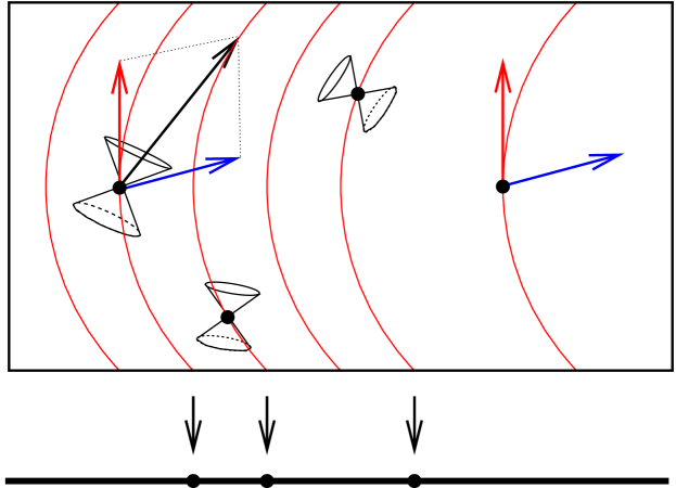
The foregoing shows that indeed defines a metric at for Ricci-positive Einstein geometries . How does the signature of this metric compare to the signature at Ricci-negative geometries? The answer is surprising: Take, e.g., for the round geometry on . Then it can be shown that defines a Lorentz geometry on , that is with signature , containing exactly one negative direction Giulini:1995c . This means that the signature of the metric defined at various points in Superspace varies strongly, with intermediate transition regions where no metric can be defined at all due to signature change. Figure 1 is an attempt to picture this situation.
4 Intermezzo: GR as simplest representation of symmetry
It is well known that the field equations of GR have certain uniqueness properties and can accordingly be ‘deduced’ under suitable hypotheses involving a symmetry principle (diffeomorphism invariance), the equivalence principle, and some apparently mild technical hypotheses. More precisely, the equivalence principle suggests to only take the metric as dynamical variable ThorneLeeLightman:1973 representing the gravitational field (to which matter then couples universally), whereas diffeomorphism invariance, derivability from an invariant Lagrangian (alternatively: local energy-momentum conservation in the sense of covariant divergencelessness), dependence of the equations on the metric up to at most second derivatives, and, finally, four-dimensionality lead uniquely to the left-hand side of Einstein’s equation, including a possibly non-vanishing cosmological constant Lovelock:1972 . Here we will review how this ‘deduction’ works in the Hamiltonian setting on phase space , which goes back to Hojman.etal:1973 ; Teitelboim:1973 ; Kuchar:1973 ; Hojman.etal:1976 .
4.1 3+1 decomposition
Since the 3+1 split of Einstein’s equations has already been introduced in Claus Kiefer’s contribution I can be brief on that point. The basic idea is to first imagine a spacetime being given, where topologically is a product . Spacetime is then considered as the trajectory (history) of space in the following way: Let denote the space of smooth spacelike embeddings . We consider a curve corresponding to a one-parameter family of smooth embeddings with spacelike images. We assume the images to be mutually disjoint and moreover that , , is an embedding (it is sometimes found convenient to relax this condition, but this is of no importance here). The Lorentz manifold may now be taken as (–dependent) representative of (or at least some open part of it) on which the leaves of the above foliation simply correspond to the hypersurfaces. Let denote a field of normalised timelike vectors normal to these leaves. is unique up to orientation, so that the choice of amounts to picking a ‘future direction’.
The tangent vector at corresponds to a vector field over (i.e. section in ), given by
| (18) |
with components normal and tangential to .
Conversely, each vector field on defines a vector field on , corresponding to the left action of on by composition. In local coordinates on and on it can be written as
| (19) |
One easily verifies that is a Lie homomorphism:
| (20) |
In this sense, the Lie algebra of the four-dimensional diffeomorphism group is implemented on phase space of any generally covariant theory whose phase space includes the embedding variables Isham.Kuchar:1985a (so-called ‘parametrised theories’).
Alternatively, decomposing (19) into normal and tangential components with respect to the leaves of the embedding at which the tangent-vector field to is evaluated, yields an embedding-dependent parametrisation of in terms of ,
| (21) |
where in square brackets indicates the functional dependence of on the embedding. The functional derivatives of with respect to can be computed (see the Appendix of Teitelboim:1973 ) and the commutator of deformation generators then follows to be,
| (22) |
where
| (23a) | |||||
| (23b) | |||||
Here we left open whether spacetime is Lorentzian () or Euclidean (), just in order to keep track how the signature of spacetime, , enters. Note that the -dependent gradient field for the scalar function is given by . The geometric idea behind (23) is summarised in Figure 2.

4.2 Hamiltonian geometrodynamics
The idea of Hamiltonian Geometrodynamics is to realise these relations in terms of a Hamiltonian system on the phase space of physical fields. The most simple case is that where the latter merely include the spatial metric on , so that the phase space is the cotangent bundle over . One then seeks a correspondence
| (24) |
where
| (25) |
with integrands and yet to be determined. should be regarded as distribution (here the test functions are and ) with values in real-valued functions on . Now, the essential requirement is that the Poisson brackets between the are, up to a minus sign,555Due to the standard convention that the Hamiltonian action being defined as a left action, whereas the Lie bracket on a group is defined by the commutator of left-invariant vector fields which generate right translations. as in (23):
| (26) |
Once the distribution satisfying (26) has been found, we can turn around the arguments given above and recover the action of the Lie algebra of four-dimensional diffeomorphism on the extended phase space including embedding variables Isham.Kuchar:1985b . That such an extension is indeed necessary has been shown in Pons:2003 , where obstructions against the implementation of the action of the Lie algebra of four-dimensional diffeomorphisms have been identified in case the dynamical fields include non-scalar ones.
4.3 Why constraints
From this follows a remarkable uniqueness result. Before stating it with all its hypotheses, we show why the constraints and must be imposed.
Consider the set of smooth real-valued functions on phase space, . They are acted upon by all via Poisson bracketing: . This defines a map from into the derivations of phase-space functions. We require this map to also respect the commutation relation (26), that is, we require
| (27) |
The subtle point to be observed here is the following: Up to now the parameters and were considered as given functions of , independent of the fields and , i.e. independent of the point of phase space. However, from (23b) we see that does depend on . This dependence may not give rise to extra terms in the Poisson bracket, for, otherwise, the extra terms would prevent the map from being a homomorphism from the algebraic structure of hypersurface deformations into the derivations of phase-space functions. This is necessary in order to interpret as a generator (on phase-space functions) of a spacetime evolution corresponding to a normal lapse and tangential shift . In other words, the evolution of observables from an initial hypersurface to a final hypersurface must be independent of the intermediate foliation (‘integrability’ or ‘path independence’ Teitelboim:1973 ; Hojman.etal:1973 ; Hojman.etal:1976 ). Therefore we placed the parameters outside the Poisson bracket on the right-hand side of (27), to indicate that no differentiation with respect to should act on them.
To see that this requirement implies the constraints, rewrite the left-hand side of (27) in the form
| (28) |
where the first equality follows from the Jacobi identity, the second from (26), and the third from the Leibniz rule. Hence the requirement (27) is equivalent to
| (29) |
for all phase-space functions to be considered and all of the form (23). Since only depends on phase space, more precisely on , this implies the vanishing of the phase-space functions for all and all of the form (23b). This can be shown to imply , i.e. . Now, in turn, for this to be preserved under all evolutions we need , and hence in particular for all , which implies , i.e. . So we see that the constraints indeed follow.
Sometimes the constraints are split into the Hamiltonian (or scalar) constraints, , and the diffeomorphisms (or vector) constraints, . The relations (26) with (23) then show that the vector constraints form a Lie-subalgebra which, because of , is not an ideal. This means that the Hamiltonian vector fields for the scalar constraints are not tangent to the surface of vanishing vector constraints, except where it intersects the surface of vanishing scalar constraints. This implies that the scalar constraints do not act on the solution space for the vector constraints, so that one simply cannot first reduce the vector constraints and then, on the solutions of that, search for solutions to the scalar constraints. Also, it is sometimes argued that the scalar constraints should not be regarded as generators of gauge transformations but rather as generators of physically meaningful motions whose effect is to change the physical state in a fashion that is, in principle, observable. See Kuchar:1993 and also Barbour.Foster:2008 and Sect. 2.3 of Claus Kiefer’s contribution for a recent revival of that discussion. However, it seems inconsistent to me to simultaneously assume 1) physical states to always satisfy the scalar constraints and 2) physical observables to exist which do not Poisson commute with the scalar constraints: The Hamiltonian vector field corresponding to such an ‘observable’ will not be tangent to the surface of vanishing scalar constraints and hence will transform physical to unphysical states upon being actually measured.
4.4 Uniqueness of Einstein’s geometrodynamics
It is sometimes stated that the relations (26) together with (23) determine the function , i.e. the integrands and , uniquely up to two free parameters, which may be identified with the gravitational and the cosmological constants. This is a mathematical overstatement if read literally, since the result can only be shown if certain additional assumptions are made concerning the action of on the basic variables and .
The first such assumption concerns the intended (‘semantic’ or ‘physical’) meaning of , namely that the action of on or is that of an infinitesimal spatial diffeomorphism of . Hence it should be the spatial Lie derivative, , applied to or . It then follows from the general Hamiltonian theory that is given by the momentum map that maps the vector field (viewed as element of the Lie algebra of the group of spatial diffeomorphisms) into the function on phase space given by the contraction of the momentum with the -induced vector field on :
| (30) |
Comparison with (25) yields
| (31) |
The second assumption concerns the intended (‘semantic’ or ‘physical’) meaning of , namely that acting on or is that of an infinitesimal ‘timelike’ diffeomorphism of normal to the leaves . If were given, it is easy to prove that we would have , where is the timelike field of normals to the leaves and is their extrinsic curvature. Hence one requires
| (32) |
Note that both sides are symmetric covariant tensor fields over . The important fact to be observed here is that appears without differentiation. This means that is an ultralocal functional of , which is further assumed to be a polynomial. (Note that we do not assume any relation between and at this point).
Quite generally, we wish to stress the importance of such ’semantic’ assumptions concerning the intended meanings of symmetry operations when it comes to ‘derivations’ of physical laws from ‘symmetry principles’. Such derivations often suffer from the same sort of overstatement that tends to give the impression that the mere requirement that some group acts as symmetries alone distinguishes some dynamical laws from others. Often, however, additional assumptions are made that severely restrict the form in which is allowed to act. For example, in field theory, the requirement of locality often enters decisively, like in the statement that Maxwell’s vacuum equations are Poincaré- but not Galilei invariant. In fact, without locality the Galilei group, too, is a symmetry group of vacuum electrodynamics Fushchich.Shtelen:1991 . Coming back to the case at hand, I do not know of a uniqueness result that does not make the assumptions concerning the spacetime interpretation of the generators . Compare also the related discussion in Samuel:2000b ; Samuel:2000a .
The uniqueness result for Einstein’s equation, which in its space-time form is spelled out in Lovelock’s theorem Lovelock:1972 already mentioned above, now takes the following form in Geometrodynamics Kuchar:1973 :
Theorem 4.1
In four spacetime dimensions (Lorentzian for , Euclidean for ), the most general functional (25) satisfying (26) with (23), subject to the conditions discussed above, is given by (31) and the two-parameter family
| (33) |
where
| (34) |
and is the Ricci scalar of . Note that (34) is just the “contravariant version” of the metric (9c) for , i.e., .
The Hamiltonian evolution so obtained is precisely that of General Relativity (without matter) with gravitational constant and cosmological constant . The proof of the theorem is given in Kuchar:1973 , which improves on earlier versions Teitelboim:1973 ; Hojman.etal:1976 in that the latter assumes in addition that be an even function of , corresponding to the requirement of time reversibility of the generated evolution. This was overcome in Kuchar:1973 by the clever move to write the condition set by (the right-hand side being already known) on in terms of the corresponding Lagrangian functional , which is then immediately seen to turn into a condition which is linear in , so that terms with even powers in velocity decouple form those with odd powers. However, a small topological subtlety remains that is neglected in all these references and which potentially introduces a little more ambiguity that that encoded in the two parameters and , though its significance is more in the quantum theory. To see this recall that we can always perform a canonical transformation of the form
| (35) |
where is a closed one-form on . The latter condition ensures that all Poisson brackets remain the same if is replaced with . Since is an open positive convex cone in a vector space and hence contractible, it is immediate that for some function . However, and must satisfy the diffeomorphism constraint, which is equivalent to saying that the kernel of (considered as one-form on ) contains the vertical vector fields, which implies that , too, must annihilate all so that is constant on each connected component of the orbit in . But unless the orbits in are connected, this does not mean that is the pull back of a function on Superspace, as assumed in Kuchar:1973 . We can only conclude that is the pull back of a closed but not necessarily exact one-form on Superspace. Hence there is an analogue of the Bohm-Aharonov-like ambiguity that one always encounters if the configuration space is not simply connected. Whether this is the case depends in a determinate fashion on the topology of : One has, due to the contractibility of ,
| (36) |
For the right hand side is
| (37) |
where is the identity component of and where we introduced the name (Mapping-Class Group for Frame fixing diffeomorphisms) for the quotient group of components.
In view of the uniqueness result above, one might wonder what goes wrong when using (the contravariant version of) the metric for in (34). The answer is that it would spoil (26). More precisely, it would contradict due to an extra term in , unless the additional constraint were imposed, which is equivalent to and hence to the condition that only maximal slices are allowed Giulini:1995c . But this is clearly unacceptable (cf. Sect. 6 of Barbour.etal:2002 ).
As a final comment about uniqueness of representations of (26) we mention the apparently larger ambiguity—labelled by an additional -valued parameter, the Barbero-Immirzi parameter—that one gets if one uses connection variables rather than metric variables (cf. Barbero:1995 ; Immirzi:1997 , Sect. 4.2.2 of Thiemann:MCQGR , and Sect. 4.3.1 of Kiefer:QuantumGravity ). However, in this case one does not represent (26) but a semi-direct product of it with the Lie algebra of gauge transformations, so that after taking the quotient with respect to the latter (which form an ideal) our original (26) is represented non locally. Also, unless the Barbero-Immirzi parameter takes the very special values (for Lorentzian signature; for Euclidean signature) the connection variable does not admit an interpretation as a space-time gauge field restricted to spacelike hypersurfaces (cf. Immirzi:1997 ; Samuel:2000a ). For example, the holonomy of a spacelike curve varies with the choice of the spacelike hypersurface containing , which would be impossible if the spatial connection were the restriction of a space-time connection Samuel:2000a . Accordingly, the dynamics generated by the constraints does then not admit the interpretation of being induced by appropriately moving a hypersurface through a spacetime with fixed geometric structures on it. Consequently, the argument provided here for why one should require (26) in the first place does, strictly speaking, not seem to apply in case of connection variables. It is therefore presently unclear to me on what set of assumptions a uniqueness result could be based in this case.
5 Topology of configuration space
Much of the global topology of is encoded in its homotopy groups, which, in turn are given by those of according to (36). Their structures were investigated in Witt:1986b ; Giulini:1995a ; Giulini:1997a . Early references as to their possible relevance in quantum gravity are Friedman.Sorkin:1980 ; Isham:1982 ; Sorkin:1986 ; Sorkin:1989 .
We start by remarking that topological invariants of are also topological invariants of , which need not be homotopy invariant of even if they are homotopy invariants of . This is, e.g., the case for the mapping-class group of homeomorphisms McCarty:1963 and hence (in 3 dimensions) also for the mapping-class group . Remarkably, this means that we may distinguish homotopy equivalent but non homeomorphic 3-manifolds by looking at homotopy invariants of their associated Superspaces. Examples for this are given by certain types of lens spaces. First recall the definition of lens spaces in 3 dimensions: , where is a pair of positive coprime integers with , , and , and . One way to picture them is to take a solid ball in and identify each point on the upper hemisphere with a points on the lower hemisphere after a rotation by about the vertical symmetry axis. (Usually one depicts the ball in a way in which it is slightly squashed along the vertical axis so that the equator develops a sharp edge and the whole body looks like a lens; see e.g. Fig. in Seifert.Threlfall:Topology .) In this way each set of equidistant points on the equator is identified to a single point. The fundamental group of is , independent of , and the higher homotopy groups are those of its universal cover, . Moreover, for connected closed orientable 3-manifolds the homology and cohomology groups are also determined by the fundamental group in an easy fashion: If denotes the operation of abelianisation of a group, the operation of taking the free part of a finitely generated abelian group, then the first four (zeroth to third, the only non-trivial ones) homology and cohomology groups are respectively given by and respectively. Hence, if taken of , all these standard invariants are sensitive only to . However, it is known that and are
-
1.
homotopy equivalent iff for some integer ,
-
2.
homeomorphic iff (all four possibilities) , and
-
3.
orientation-preserving homeomorphic iff .
The first statement is Theorem 10 in Whitehead:1941 and the second and third statement follow, e.g., from the like combinatorial classification of lens spaces Reidemeister:1935 together with the validity of the ‘Hauptvermutung’ (the equivalence of the combinatorial and topological classifications) in 3 dimensions Moise:1952 . So, for example, is homotopy equivalent but not homeomorphic to . On the other hand, it is known that the mapping-class group for is if with , which applies to and , and that in the remaining cases for it is just (see Table IV on p. 591 of Witt:1986b ). Hence for and for , even though and are homotopy equivalent!
Quite generally it turns out that Superspace stores much information about the topology of the underlying 3-manifold . This can be seen from the table in Figure 3, which we reproduced form Giulini:1994a , and where properties of certain prime manifolds (see below for an explanation of ‘prime’) are listed. There is one interesting observation from that list which we shall mention right away: From gauge theories it is known that there is a relation between topological invariants of the classical configuration space and certain features of the corresponding quantum-field theory Jackiw:LesHouches1983 , in particular the emergence of certain anomalies which represent non-trivial topological invariants Alvarez-GaumeGinsparg:1985 . By analogy one could conjecture similar relations to hold quantum gravity. An interesting question is then whether there are preferred manifolds for which all these invariants are trivial. From those represented on the table there is indeed a unique pair of manifolds for which this is the case, namely the 3-sphere and the 3-dimensional real projective space. To understand more of the information collected in the table we have to say more about general 3-manifolds.
Of particular interest is the fundamental group of Superspace. Experience with ordinary quantum mechanics (cf. Giulini:1995b and references therein) already suggests that its classes of inequivalent irreducible unitary representations correspond to a superselection structure which here might serve as fingerprint of the topology of in the quantum theory. The sectors might, e.g., correspond to various statistics (in the presence of diffeomorphic primes) that preserve or violate a naively expected spin-statistics correlation Aneziris.etal:1989a ; Aneziris.etal:1989b ; Dowker.Sorkin:1998 ; Dowker.Sorkin:2000 (see also below).
5.1 General three-manifolds and specific examples

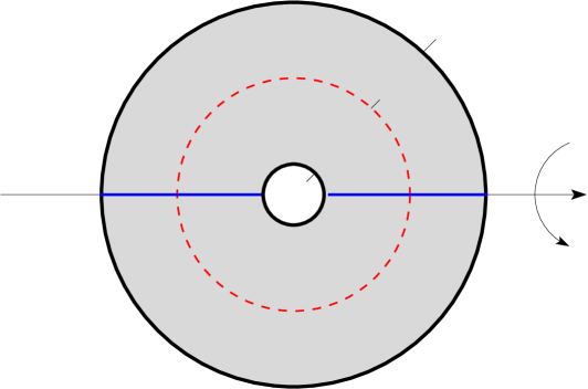
The way to understand general 3-manifolds is by cutting them along certain embedded two manifolds so that the remaining pieces are simpler in an appropriate sense. Here we shall only consider those simplifications that are achieved by cutting along embedded 2-spheres. (Further decompositions by cutting along 2-tori provide further simplifications, but these are not directly relevant here.) The 2-spheres should be ‘essential’ and ‘splitting’. An essential 2-sphere is one which does not bound a 3-ball and a splitting 2-sphere is one whose complement has two (rather than just one) connected components. Figure 4 is intended to visualise the analogues of these notions in two dimensions.
Given a closed 3-manifold , consider the following process: Cut it along an essential splitting 2-sphere and cap off the 2-sphere boundary of each remaining component by a 3-disk. Now repeat the process for each of the remaining closed 3-manifolds. This process stops after a finite number of steps Kneser:1929 where the resulting components are uniquely determined up to diffeomorphisms (orientation preserving if oriented manifolds are considered) and permutation Milnor:1962 ; see Hatcher:3-manifolds for a lucid discussion. The process stops at that stage at which none of the remaining components, , allows for essential splitting 2-spheres, i.e. at which each is a prime manifold. A 3-manifold is called prime if each embedded 2-sphere either bounds a 3-disc or does not split; it is called irreducible if each embedded 2-sphere bounds a 3-disc. In the latter case the second homotopy group, , must be trivial, since, if it were not, the so-called sphere theorem (see, e.g., Hatcher:3-manifolds ) ensured the existence of a non-trivial element of which could be represented by an embedded 2-sphere. Conversely, it follows from the validity of the Poincaré conjecture that a trivial implies irreducibility. Hence irreducibility is equivalent to a trivial . There is precisely one non-irreducible prime 3-manifold, and that is the handle . Hence a 3-manifold is prime iff it is either a handle or if its is trivial.
Given a general 3-manifold as connected sum of primes , there is a general method to establish in terms of the individual mapping-class groups of the primes. The strategy is to look at the effect of elements in on the fundamental group of . As is the connected sum of primes, and as connected sums in dimensions are taken along spheres which are simply-connected for , the fundamental group of a connected sum is the free product of the fundamental groups of the primes for . The group now naturally acts as automorphisms of by simply taking the image of a based loop that represents an element in by a based (same basepoint) diffeomorphism that represents the class in . Hence there is a natural map
| (38) |
The known presentations666A (finite) presentation of a group is its characterisation in terms of (finitely many) generators and (finitely many) relations. of automorphism groups of free products in terms of presentations of the automorphisms of the individual factors and additional generators (basically exchanging isomorphic factors and conjugating whole factors by individual elements of others) can now be used to establish (finite) presentations of , provided (finite) presentations for all prime factors are known.777This presentation of the automorphism group of free products is originally due to Fouxe-Rabinovitch Fouxe-Rabinovitch:1940 ; Fouxe-Rabinovitch:1941 . Modern forms with corrections are given in McCullough.Miller:1986 and Gilbert:1987 Here I wish to stress that this situation would be more complicated if rather than (or at least the diffeomorphisms fixing a preferred point) had been considered; that is, had we not made the transition from (1) to (4). Only for (or the slightly larger group of diffeomorphisms fixing the point) is it generally true that the mapping-class group of a prime factor injects into the mapping-class group of the connected sum in which it appears. For more on this, compare the discussion on p. 182-3 in Giulini:2007a . Clearly, one also needs to know which elements are in the kernel of the map (38). This will be commented on below in connection with Fig 7.


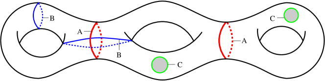
5.2 The connected sum of two real-projective spaces
In some (in fact many) cases the map is an isomorphism. For example, this is the case if is the connected sum of two , so that is the free product , a presentation of which is . For the automorphisms we have , where and . In this sense the infinite discrete group is a quotient of the automorphism group of Superspace for being the connected sum of two real projective spaces. It is therefore of interest to study its unitary irreducible representations. This can be done directly in a rather elementary fashion, or more systematically by a simple application of the method of induced representations (Mackey theory) using the isomorphicity (cf. caption to Fig. 6). The result is that, apart form the obvious four one-dimensional ones, given by , there is a continuous set of mutually inequivalent two-dimensional ones, given by
| (39) |
Already in this most simple example of a non-trivial connected sum we have an interesting structure in which the two ‘statistics sectors’ corresponding to the irreducible representations of the permutation subgroup (here just given by the subgroup generated by ) get mixed by , where the ‘mixing angle’ uniquely characterises the representation. This behaviour can also be studied in more complicated examples Giulini:1994a SorkinSurya:1998 . For a more geometric understanding of the maps representing and , see Giulini:2007a .

5.3 Spinoriality
I also wish to mention one very surprising observation that was made by Rafael Sorkin and John Friedman in 1980 Friedman.Sorkin:1980 and which has to do with the physical interpretation of the elements in the kernel of the map (38), leading to the conclusion that pure (i.e. without matter) quantum gravity should already contain states with half-integer angular momenta. The reason being a purely topological one, depending entirely on the topology of . In fact, given the right topology of , its one-point decompactification used in the context of asymptotically flat initial data will describe an isolated system whose asymptotic (at spacelike infinity) symmetry group is not the ordinary Poincaré group Beig.Murchadha:1987 but rather its double (= universal) cover. This gives an intriguing answer to Wheeler’s quest to find a natural place for spin 1/2 in Einstein’s standard geometrodynamics (cf. Misner.Thorne.Wheeler:Gravitation Box 44.3).
I briefly recall that after introducing the concept of a ‘Geon’ (‘gravitational-electromagnetic entity’) in 1955 Wheeler:1955 , and inspired by the observation that electric charge (in the sense of non-vanishing flux integrals of over closed 2-dimensional surfaces) could be realised in Einstein-Maxwell theory without sources (‘charge without charge’), Wheeler and collaborators turned to the Einstein-Weyl theory Brill.Wheeler:1957 and tried to find a ‘neutrino analog of electric charge’ Klauder.Wheeler:1957 . Though this last attempt failed, the programme of ‘matter as geometry’ in the context of geometrodynamics, as outlined in the contributions to the anthology Wheeler:Geometrodynamics , survived in Wheeler’s thinking well into the 1980s Wheeler:1982 .
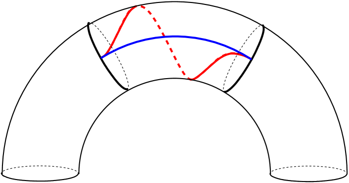
Back to the ‘spin without spin’ topologies, the elements of the kernel of (38) can be pictured as rotation parallel to certain spheres, as depicted in Figure 7. (In many—and possibly all—cases the group generated by such maps actually exhaust the kernel; compare Theorem. 1.5 in McCullough:1990 and footnote 21 in Giulini:2007a ). The point we wish to focus on here is that for some prime manifolds the diffeomorphism depicted on the left in Figure 7 is indeed not in the identity component of all diffeomorphisms that fix a frame exterior to the outer () 2-sphere. Such manifolds are called spinorial. For each prime it is known whether it is spinorial or not, and the easy-to-state but hard-to-prove result is, that the only non-spinorial manifolds888 We remind the reader that ‘manifold’ here stands for ‘3-dimensional closed orientable manifold’. are the lens spaces , the handle , and connected sums amongst them. That these manifolds are not spinorial is, in fact, very easy to visualise. Hence, given the proof of the ‘only’ part and of the fact that a connected sum is spinorial iff it contains at least one spinorial prime, one may summarise the situation by saying that that the only non-spinorial manifolds are the ‘obvious’ ones.
Even though being a generic property in the sense just stated, spinoriality is generally hard to prove in dimensions three or greater. This is in marked contrast to two dimensions, where the corresponding transformation shown in the left picture of Figure 7 acts non trivially on the fundamental group. Indeed, consider a base point outside (below) in the left picture in Figure 7, then the rotation acts by conjugating each of the generators that adds to by the element , which is non-trivial in if other primes exist or otherwise if the point with the fixed frame is removed (as one may do, due to the restriction to diffeomorphisms fixing that point).
An example of a spinorial manifold is the spherical space form , where is thought of as the sphere of unit quaternions and is the subgroup in the group of unit quaternions given by the eight elements . The coset space may be visualised as solid cube whose opposite faces are identified after a -degree rotation by either a right- or a left-handed screw motion; see Figure 8. Drawings of fundamental domains in form of (partially truncated) solid polyhedra with suitable boundary identifications for spaces are given in DuVal:Homographies .
Let us take the basepoint to be the centre of the cube in Figure 8. The two generators, and , of the fundamental group
| (40) |
are then represented by two of the three oriented straight segments connecting the midpoints of opposite faces. The third corresponds to the product . A rotation of the cube about its centre by any element of its crystallographic symmetry group defines a diffeomorphism of fixing since it is compatible with the boundary identification. It is not in the identity component of -fixing diffeomorphisms since it obviously acts non-trivially on the generators of the fundamental group. Clearly, each such rigid rotation may be modified in an arbitrarily small neighbourhood of so as to also fix the tangent space at this point. That is spinorial means that in going from the point-fixing to the frame-fixing diffeomorphisms one acquires more diffeomorphisms not connected to the identity. More precisely, the mapping-class group of frame-fixing diffeomorphisms is a -extension of the mapping-class group of merely point-fixing diffeomorphisms. The generator of this extending is a full -degree rotation parallel to two small concentric spheres centred at . In this way, the spinoriality of extends the crystallographic symmetry group of the cube to its double cover and one finally gets
| (41) |
This is precisely what one finds at the intersection of the 2nd row and 7th column of the table in Figure 3, with corresponding results for the other spherical space forms.
Coming back to the previous example of the connected sum of two (or more Giulini:1994a ) real projective spaces, we can make the following observation: First of all, real projective 3-space is a non-spinorial prime. This is obvious once one visualises it as a solid 3-ball whose 2-sphere boundary points are pairwise identified in an antipodal fashion, since this identification is compatible with a rigid rotation. A full rotation about the, say, centre-point of the ball may therefore be continuously undone by a rigid rotation outside a small ball about the centre, suitably ‘bumped off’ towards the centre. Second, as we have seen above, the irreducible representations of the mapping-class group of the connected sum contains both statistics sectors independently for one-dimensional representations and in a mixed form for the continuum of two-dimensional irreducible representations. This already shows Aneziris.etal:1989b that there is no general kinematical spin-statistics relation as in other non-linear theories Finkelstein.Rubinstein:1968 ; Sorkin:1988 . Such a relation may at best be re-introduced for some manifolds by restricting the way in which states are constructed, e.g., via the sum-over-histories approach Dowker.Sorkin:1998 .
5.4 Chirality
There is one last aspect about diffeomorphisms that can be explained in terms of Figure 8. As stated in the caption of this figure, there are two versions of this space: one where the identification of opposite faces is done via a -degree right-handed screw motion and one where one uses a left-handed screw motion. These spaces are not related by an orientation preserving diffeomorphism. This is equivalent to saying that, say, the first of these spaces has no orientation-reversing self-diffeomorphism. Manifolds for which this is the case are called chiral. There are no examples in two dimensions. To see this, just consider the usual picture of a Riemannian genus surface embedded into and map it onto itself by a reflection at any of its planes of symmetry. So chiral manifolds start to exist in 3 dimensions and continue to do so in all higher dimensions, as was just recently shown Muellner:2008 . If one tries to reflect the cube in Figure 8 at one of its symmetry planes one finds that this is incompatible with the boundary identifications, that is, pairs of identified points are not mapped to pairs of identified points. Hence this reflection simply does not define a map of the quotient space. This clearly does not prove the nonexistence of orientation reversing maps, since there could be others than these obvious candidates.
In fact, following an idea of proof in Witt:1986b , the chirality of (and others of the form ) can be reduced to that of . That the latter is chiral follows from the following argument: Above we have already stated that and are orientation preserving diffeomorphic iff . Since taking the mirror image in of the lens representing gives the lens representing , admits an orientation reversing diffeomorphism iff and are orientation preserving diffeomorphic. But, as just stated, this is the case iff , i.e. if either (recall that and must be coprime) or .999Remarkably, this result was already stated in footnote 1 of p. 256 of Kneser:1929 . An early published proof is that in Sect. 77 of Seifert.Threlfall:Topology Hence, in particular, all are chiral. Now, has three subgroups isomorphic to , the fundamental group of , namely the ones generated by , , and . They are normal so that we have a regular covering . Now suppose were orientation reversing, i.e. a diffeomorphism with . Consider the diagram
| (42) |
If the lift existed we would immediately get a contradiction since from commutativity of (42) we would get and hence , which contradicts chirality of . Now, according to the theory of covering spaces the lift of exists iff the image of under , which is a subgroup , is conjugate to the image of under . This need not be the case, however, as different subgroups in are normal and hence never conjugate (here we deviate from the argument in Witt:1986b which seems incorrect). However, by composing a given orientation reversing with an orientation preserving diffeomorphism that undoes the subgroup permutation introduced by , we can always create a new orientation reversing diffeomorphism that does not permute the subgroups. That new orientation reversing diffeomorphism—call it again —now indeed has a lift , so that finally we arrive at the contradiction envisaged above.
As prime manifolds, the two versions of a chiral prime corresponding to the two different orientations count as different. This means the following: Two connected sums which differ only insofar as a particular chiral prime enters with different orientations are not orientation-preserving diffeomorphic; they are not diffeomorphic at all if the complement of the selected chiral prime also chiral (i.e. iff another chiral prime exists). For example, the connected sum of two oriented is not diffeomorphic to the connected sum of with , where the overbar indicates the opposite orientation. Note that the latter case also leads to two non-homeomorphic 3-manifolds whose classic invariants (homotopy, homology, cohomology) coincide. This provides an example of a topological feature of that is not encoded into the structure of .
6 Summary and outlook
Superspace is for geometrodynamics what gauge-orbit space is for non-abelian gauge theories, though Superspace has generally a much richer topological and metric structure. Its topological structure encodes much of the topology of the underlying 3-manifold and one may conjecture that some of its topological invariants bear the same relation to anomalies and sectorial structure as in the case of non-abelian gauge theories. Recent progress in 3-manifold theory now allows to make more complete statements, in particular concerning the fundamental groups of Superspaces associated to more complicated 3-manifolds. Its metric structure is piecewise nice but also suffers from singularities, corresponding to signature changes, whose physical significance is unclear. Even for simple 3-manifolds, like the 3-sphere, there are regions in superspace where the metric is strictly Lorentzian (just one negative signature and infinitely many pluses), like at the round 3-sphere used in the FLRW cosmological models, so that the Wheeler-DeWitt equation becomes strictly hyperbolic, but there are also regions with infinitely many negative signs in the signature.
Note that the cotangent bundle over Superspace is not the fully reduced phase space for matter-free General Relativity. It only takes account of the vector constraints and leaves the scalar constraint unreduced. However, under certain conditions, the scalar constraints can be solved by the ‘conformal method’ which leaves only the conformal equivalence class of 3-dimensional geometries as physical configurations. In those cases the fully reduced phase space is the cotangent bundle over conformal superspace, whose analog to (1) is given by replacing by the semi-direct product , where is the abelian group of conformal rescalings that acts on via (pointwise multiplication), where . The right action of on is then given by by , so that, using , the semi-direct product structure is seen to be . Note that because of indeed acts as automorphisms of . Conformal superspace and extended conformal superspace would then, in analogy to (1) and (4), be defined as and respectively. The first definition was used in Fischer.Moncrief:1996 as applied to manifolds with zero degree of symmetry (cf. footnote 3). In any case, since is contractible, the topologies of and are those of and which also transcend to the quotient spaces analogously to (36) whenever the groups act freely. In the first case this is essentially achieved by restricting to manifolds of vanishing degree of symmetry, whereas in the second case this follows almost as before, with the sole exception being with conformal to the round metric.101010 Let be the group of conformal isometries. For compact it is known to be compact except iff and conformal to the round metric Lelong-Ferrand:1971 . Hence, for , we can average over the compact group and obtain a new Riemannian metric in the conformal equivalence class of for which acts as proper isometries. Therefore, by the argument presented in Sect.2, it cannot contain non-trivial elements fixing a frame. Hence the topological results obtained before also apply to this case. In contrast, the geometry for conformal superspace differs insofar from that discussed above as the conformal modes that formed the negative directions of the Wheeler-DeWitt metric (cf. (9a) are now absent. The horizontal subspaces (orthogonal to the orbits of ) are now given by the transverse and traceless (rather than just obeying (13)) symmetric two-tensors. In that sense the geometry of conformal superspace, if defined as before by some ultralocal bilinear form on , is manifestly positive (due to the absence of trace terms) and hence less pathological than the superspace metric discussed above. It might seem that its physical significance is less clear, as there is now no constraint left that may be said to induce this particular geometry; see however Barbour.Murchadha:1999 .
Whether it is a realistic hope to understand superspace and conformal superspace (its cotangent bundle being the space of solutions to Einstein’s equations) well enough to actually gain a sufficiently complete understanding of its automorphism group is hard to say. An interesting strategy lies in the attempt to understand the solution space directly in a group- (or Lie algebra-) theoretic fashion in terms of a quotient , where is an infinite dimensional group (Lie algebra) that (locally) acts transitively on the space of solutions and is a suitable subgroup (algebra), usually the fixed-point set of an involutive automorphism of . The basis for the hope that this might work in general is the fact that it works for the subset of stationary and axially symmetric solutions, where is the Geroch Group; cf. Breitenlohner.Maison:1987 . The idea for generalisation, even to supergravity, is expressed in Nicolai:1999 and further developed in Damour.etal:2007 .
Acknowledgements I thank Hermann Nicolai and Stefan Theisen for inviting me to this stimulating 405th WE-Heraeus-Seminar on Quantum Gravity and for giving me the opportunity to contribute this paper. I also thank Hermann Nicolai for pointing out Nicolai:1999 and Ulrich Pinkall for pointing out Lelong-Ferrand:1971 .
References
- [1] Luis Alvarez-Gaumé and Paul Ginsparg. The structure of gauge and gravitational anomalies. Annals of Physics, 161:423–490, 1985.
- [2] Charilaos Aneziris et al. Aspects of spin and statistics in general covariant theories. International Journal of Modern Physics A, 14(20):5459–5510, 1989.
- [3] Charilaos Aneziris et al. Statistics and general relativity. Modern Physics Letters A, 4(4):331–338, 1989.
- [4] Richard Arens. Classical Lorentz invariant particles. Journal of Mathematical Physics, 12(12):2415–2422, 1971.
- [5] Henri Bacry. Space-time and degrees of freedom of the elementary particle. Communications in Mathematical Physics, 5(2):97–105, 1967.
- [6] Fernando Barbero. Real Ashtekar variables for Lorentzian signature space-times. Physical Review D, 51(10):5507–5510, 1995.
- [7] Julian Barbour and Brendan Z Foster. Constraints and gauge transformations: Dirac’s theorem is not always valid. arXiv:0808.1223v1, 2008.
- [8] Julian Barbour, Brendan Z. Foster, and Niall Ó Murchadha. Relativity without relativity. Classical and Quantum Gravity, 19(12):3217–3248, 2002.
- [9] Julian Barbour and Niall Ó Murchadha. Classical and quantum gravity on conformal superspace. arXiv:gr-qc/9911071v1, 1999.
- [10] Robert Beig and Niall Ó Murchadha. The Poincaré group as symmetry group of canonical general relativity. Annals of Physics, 174:463–498, 1987.
- [11] Arthur L. Besse. Einstein Manifolds. Ergebnisse der Mathematik und ihrer Grenzgebiete, 3. Folge Band 10. Springer Verlag, Berlin, 1987.
- [12] Peter Breitenlohner and Dieter Maison. On the Geroch group. Annales de l’Institut Henri Poincaré, Section A, 46(2):215–246, 1987.
- [13] Dieter R. Brill and John A. Wheeler. Interaction of neutrinos and gravitational fields. Review of Modern Physics, 29(3):465–479, 1957.
- [14] Thibault Damour, Axel Kleinschmidt, and Hermann Nicolai. Constraints and the coset model. Classical and Quantum Gravity, 24(23):6097–6120, 2007.
- [15] Thibault Damour and Hermann Nicolai. Symmetries, singularities and the de-emergence of space. arXiv:0705.2643v1, 2007.
- [16] Bryce Seligman DeWitt. Quantum theory of gravity. I. The canonical theory. Physical Review, 160(5):1113–1148, 1967. Erratum, ibid. 171(5):1834, 1968.
- [17] Fay Dowker and Rafael Sorkin. A spin-statistics theorem for certain topological geons. Classical and Quantum Gravity, 15:1153–1167, 1998.
- [18] Fay Dowker and Rafael Sorkin. Spin and statistics in quantum gravity. In R.C. Hilborn and G.M. Tino, editors, Spin-Statistics Connections and Commutation Relations: Experimental Tests and Theoretical Implications, pages 205–218. American Institute of Physics, New York, 2000.
- [19] Patrick Du Val. Homographies, Quaternions, and Rotations. Clarendon Press, Oxford, 1964.
- [20] David G. Ebin. On the space of Riemannian metrics. Bulletin of the American Mathematical Society, 74(5):1001–1003, 1968.
- [21] David Finkelstein and Julio Rubinstein. Connection between spin, statistics, and kinks. Journal of Mathematical Physics, 9(11):1762–1779, 1968.
- [22] Arthur E. Fischer. The theory of superspace. In M. Carmeli, S.I. Fickler, and L. Witten, editors, Relativity, proceedings of the Relativity Conference in the Midwest, held June 2-6, 1969, at Cincinnati Ohio, pages 303–357. Plenum Press, New York, 1970.
- [23] Arthur E. Fischer. Resolving the singularities in the space of Riemannian geometries. Journal of Mathematical Physics, 27:718–738, 1986.
- [24] Arthur E. Fischer and Vincent E. Moncrief. The structure of quantum conformal superspace. In S. Cotsakis and G.W. Gibbons, editors, Global Structure and Evolution in General Relativity, volume 460 of Lecture Notes in Physics, pages 111–173. Springer Verlag, Berlin, 1996.
- [25] David Izrailevich Fouxe-Rabinovitch. Über die Automorphismengruppen der freien Produkte I. Matematicheskii Sbornik, 8(50):265–276, 1940.
- [26] David Izrailevich Fouxe-Rabinovitch. Über die Automorphismengruppen der freien Produkte II. Matematicheskii Sbornik, 9(51):297–318, 1941.
- [27] Daniel S. Freed and David Groisser. The basic geometry of the manifold of Riemannian metrics and of its quotient by the diffeomorphism group. Michigan Mathematical Journal, 36(3):323–344, 1989.
- [28] John Friedman and Rafael Sorkin. Spin 1/2 from gravity. Physical Review Letters, 44:1100–1103, 1980.
- [29] Wilhelm Fushchich and Vladimir Shtelen. Are Maxwell’s equations invariant under the Galilei transformations? Doklady Akademii Nauk Ukrainy A, 3:22–26, 1991. In Russian.
- [30] L. Zhiyong Gao and Shing-Tung Yau. The existence of negatively Ricci curved metrics on three-manifolds. Inventiones Mathematicae, 85(3):637–652, 1986.
- [31] Nick D. Gilbert. Presentations of the automorphims group of a free product. Proceedings of the London Mathematical Society, 54:115–140, 1987.
- [32] Domenico Giulini. 3-manifolds for relativists. International Journal of Theoretical Physics, 33:913–930, 1994.
- [33] Domenico Giulini. On the configuration-space topology in general relativity. Helvetica Physica Acta, 68:86–111, 1995.
- [34] Domenico Giulini. Quantum mechanics on spaces with finite fundamental group. Helvetica Physica Acta, 68:439–469, 1995.
- [35] Domenico Giulini. What is the geometry of superspace? Physical Review D, 51(10):5630–5635, 1995.
- [36] Domenico Giulini. The group of large diffeomorphisms in general relativity. Banach Center Publications, 39:303–315, 1997.
- [37] Domenico Giulini. Mapping-class groups of 3-manifolds in canonical quantum gravity. In Bertfried Fauser, Jürgen Tolksdorf, and Eberhard Zeidler, editors, Quantum Gravity: Mathematical Models and Experimental Bounds. Birkhäuser Verlag, Basel, 2007. Online available at arxiv.org/pdf/gr-qc/0606066.
- [38] Domenico Giulini and Claus Kiefer. Wheeler-DeWitt metric and the attractivity of gravity. Physics Letters A, 193(1):21–24, 1994.
- [39] Allen E. Hatcher. Notes on basic 3-manifold topology. Online available at www.math.cornell.edu/hatcher/3M/3Mdownloads.html.
- [40] Sergio A. Hojman, Karel Kuchař, and Claudio Teitelboim. New approach to general relativity. Nature Physical Science, 245:97–98, October 1973.
- [41] Sergio A. Hojman, Karel Kuchař, and Claudio Teitelboim. Geometrodynamics regained. Annals of Physics, 96:88–135, 1976.
- [42] Giorgio Immirzi. Real and complex connections for canonical gravity. Classical and Quantum Gravity, 14(10):L117–L181, 1997.
- [43] Christopher J. Isham. –states induced by the diffeomorphism group in canonically quantized gravity. In J.J. Duff and C.J. Isham, editors, Quantum Structure of Space and Time, Proceedings of the Nuffield Workshop, August 3-21 1981, Imperial College London, pages 37–52. Cambridge University Press, London, 1982.
- [44] Christopher J. Isham and Karel V. Kuchař. Representations of spacetime diffeomorphisms. I. Canonical parametrized field theories. Annals of Physics, 164:288–315, 1985.
- [45] Christopher J. Isham and Karel V. Kuchař. Representations of spacetime diffeomorphisms. II. Canonical geometrodynamics. Annals of Physics, 164:316–333, 1985.
- [46] Roman Jackiw. Topological investigations of quantized gauge theories. In Bryce DeWitt and Raymond Stora, editors, Relativity, Groups, and Topology II, Les Houches, Session XL, pages 37–52. North Holland, Amsterdam, 1984.
- [47] Jerry L. Kazdan and Frank W. Warner. Scalar curvature and conformal deformation of Riemannian structure. Journal of Differential Geometry, 10(1):113–134, 1975.
- [48] Claus Kiefer. Quantum Gravity, volume 124 of International Series of Monographs on Physics. Clarendon Press, Oxford, second edition, 2007.
- [49] John Klauder and John A. Wheeler. On the question of a neutrino analog to electric charge. Reviews of Modern Physics, 29(3):516–517, 1957.
- [50] Hellmuth Kneser. Geschlossene Flächen in dreidimensionalen Mannigfaltigkeiten. Jahresberichte der deutschen Mathematiker Vereinigung, 38:248–260, 1929.
- [51] Karel Kuchař. Geometrodynamics regained: A Lagrangian approach. Journal of Mathematical Physics, 15(6):708–715, 1974.
- [52] Karel Kuchař. Canonical quantum gravity. In R.J. Gleiser, C.N. Kosameh, and O.M. Moreschi, editors, General Relativity and Gravitation, pages 119–150. IOP Publishing, Bristol, 1993.
- [53] Jacqueline Lelong-Ferrand. Transformation conformes et quasiconformes des variétés riemanniennes compacts (démonstration de la conjecture de A. Lichnerowicz). Mémoires de la Classe des Sciences de l’Académie royale des Sciences, des Lettres et des Beaux-Arts de Belgique, 39(5):3–44, 1971.
- [54] David Lovelock. The four-dimensionality of space and the Einstein tensor. Journal of Mathematical Physics, 13(6):874–876, 1972.
- [55] George Shultz McCarty. Homeotopy groups. Transactions of the American Mathematical Society, 106:293–303, 1963.
- [56] Darryl McCullough. Topological and algebraic automorphisms of 3-manifolds. In Renzo Piccinini, editor, Groups of Homotopy Equivalences and Related Topics, volume 1425 of Springer Lecture Notes in Mathematics, pages 102–113. Springer Verlag, Berlin, 1990.
- [57] Darryl McCullough and Andy Miller. Homeomorphisms of 3-manifolds with compressible boundary. Memoirs of the American Mathematical Society, 61(344), 1986.
- [58] John W. Milnor. A unique decomposition theorem for 3-manifolds. American Journal of Mathematics, 84(1):1–7, 1962.
- [59] Charles W. Misner, Kip S. Thorne, and John Archibald Wheeler. Gravitation. W.H. Freeman and Company, New York, 1973.
- [60] Edwin Evariste Moise. Affine structures in 3-manifolds V. The triangulation theorem and Hauptvermutung. Annals of Mathematics, 56(1):96–114, 1952.
- [61] Daniel Müllner. Orientation Reversal of Manifolds. PhD thesis, Friedrich-Wilhelms-Universität Bonn, October 2008.
- [62] Sumner B. Myers and Norman E. Steenrod. The group of isometries of a Riemannian manifold. Annals of Mathematics, 40(2):400–416, 1939.
- [63] Hermann Nicolai. On M-theory. Journal of Astrophysics and Astronomy, 20(3-4):149–164, 1999.
- [64] Josep M. Pons. Generally covariant theories: The Noether obstruction for realizing certain space-time diffeomorphisms in phase space. Classical and Quantum Gravity, 20(15):3279–3294, 2003.
- [65] Kurt Reidemeister. Homotopieringe und Linsenräume. Abhandlungen aus dem Mathematischen Seminar der Universität Hamburg, 11(1):102–109, 1935.
- [66] Joseph Samuel. Canonical gravity, diffeomorphisms and objective histories. Classical and Quantum Gravity, 17(22):4645–4654, 2000.
- [67] Joseph Samuel. Is Barbero’s Hamiltonian formulation a gauge theory of Lorentzian gravity? Classical and Quantum Gravity, 17(20):L141–L148, 2000.
- [68] Herbert Seifert and William Threlfall. A Textbook of Topology. Academic Press, Orlando, Florida, 1980. Translation of the 1934 german edition.
- [69] Rafael Sorkin. Introduction to topological geons. In P.G. Bergmann and V. De Sabbata, editors, Topological Properties and Global Structure of Space-Time, volume B138 of NATO Advanced Study Institutes Series, page 249. D. Reidel Publishing Company, Dordrecht-Holland, 1986.
- [70] Rafael Sorkin. A general relation between kink-exchange and kink-rotation. Communications in Mathematical Physics, 115:421–434, 1988.
- [71] Rafael Sorkin. Classical topology and quantum phases: Quantum geons. In S. De Filippo, M. Marinaro, G. Marmo, and G. Vilasi, editors, Geometrical and Algebraic Aspects of Nonlinear Field Theory, pages 201–218. Elsevier Science Publishers B.V., Amsterdam, 1989.
- [72] Rafael Sorkin and Sumati Surya. An analysis of the representations of the mapping class group of a multi-geon three-manifold. International Journal of Modern Physics A, 13(21):3749–3790, 1998.
- [73] Michael D. Stern. Investigations of the Topology of Superspace. PhD thesis, Department of Physics, Princeton University, April 28th 1967.
- [74] Claudio Teitelboim. How commutators of constraints reflect the spacetime structure. Annals of Physics, 79(2):542–557, 1973.
- [75] Thomas Thiemann. Modern Canonical Quantum General Relativity. Cambridge Monographs on Mathematical Physics. Cambridge University Press, Cambridge, 2007.
- [76] Kip S. Thorne, David L. Lee, and Alan P. Lightman. Foundations for a theory of gravitation theories. Physical Review D, 7(12):563–3578, 1973.
- [77] John A. Wheeler. Geons. Physical Review, 97(2):511–536, 1955.
- [78] John A. Wheeler. Geometrodynamics. Academic Press, New York, 1962.
- [79] John A. Wheeler. Einsteins Vision. Springer Verlag, Berlin, 1968.
- [80] John A. Wheeler. Superspace and the nature of quantum geometrodynamics. In Cecile M. DeWitt and John A. Wheeler, editors, Battelle Rencontres, 1967 Lectures in Mathematics and Physics, pages 242–307. W.A. Benjamin, New York, 1968.
- [81] John A. Wheeler. Particles and geometry. In P. Breitenlohner and H.P. Dürr, editors, Unified Theories of Elementary Particles, volume 160 of Lecture Notes in Physics, pages 189–217. Springer Verlag, Berlin, 1982.
- [82] John Henry Constantine Whitehead. On incidence matrices, nuclei and homotopy types. Annals of Mathematics, 42(5):1197–1239, 1941.
- [83] Donald Witt. Symmetry groups of state vectors in canonical quantum gravity. Journal of Mathematical Physics, 27(2):573–592, 1986.
- [84] Donald Witt. Vacuum space-times that admit no maximal slices. Physical Review Letters, 57(12):1386–1389, 1986.