Fractional Fokker-Planck subdiffusion in alternating fields

Abstract

The fractional Fokker-Planck equation for subdiffusion in time-dependent force fields is derived from the underlying continuous time random walk. Its limitations are discussed and it is then applied to the study of subdiffusion under the influence of a time-periodic rectangular force. As a main result, we show that such a force does not affect the universal scaling relation between the anomalous current and diffusion when applied to the biased dynamics: in the long time limit subdiffusion current and anomalous diffusion are immune to the driving. This is in sharp contrast with the unbiased case when the subdiffusion coefficient can be strongly enhanced, i.e. a zero-frequency response to a periodic driving is present.

I Introduction

The theoretical study of anomalously slow relaxation processes in time-dependent force fields constitutes a challenge of current research interest which is not free of ambiguity. It is known that there is no unique physical mechanism responsible for the occurrence of subdiffusion in condensed media Bouchaud1990 . One possible mechanism, which will be addressed in this work, corresponds to disordered glassy-like media consisting of trapping domains where the traveling particle can dwell for a random time with divergent mean value Scher ; ScherMontroll ; shlesinger1974 . The successive residence times in traps are assumed to be mutually uncorrelated. Diffusion is nevertheless a non-Markovian (semi-Markovian) process exhibiting long (quasi-infinite) time correlations in the particle positions with a weak ergodicity breaking BelBarkai . Mathematically this physical picture can be described by a continuous time random walk (CTRW) model ScherMontroll ; shlesinger1974 which in the continuous space limit leads to the fractional Fokker-Planck equation (FFPE) metzler2000R ; letter ; heinsalu2006b . This latter formulation is incomplete, as no non-Markovian master equation can define the underlying non-Markovian stochastic process HT . However, the FFPE is very useful and has a tightly associated, complete description with (ordinary) Langevin equation in subordinated, random operational time Fogedby1994 ; Stanislavsky ; Magdziartz .

The generalization of the CTRW and FFPE to time-dependent forces is a highly non-trivial matter since the force changes in the real and not in the operational time heinsalu2007b ; goychuk07 . Also, how a field varying in time affects the distribution of the residence times in the traps is not clear without specifying a concrete mechanism or some plausible model, especially when the mean residence time does not exist PRE04 . The FFPE describing the dynamics in time-dependent force fields $F(x,t)$ becomes ambiguous with a frequently (ab)used, ad hoc version sokolov2001 ; Sample which lacks clear theoretical grounds heinsalu2007b . The correct version of the FFPE for time-dependent fields was first given in Refs. SokolovKlafter06 ; heinsalu2007b : differently from the FFPE for a time-independent force, in the case of a time-dependent field the fractional derivative does not stand in front of the Fokker-Planck operator but after it. As we explain with this work in more detail, such a FFPE can be justified beyond the linear response approximation within a CTRW approach only for a special class of dichotomously fluctuating fields. The derivation of the FFPE for subdiffusion in such time-dependent fields is presented in Sec. II.

In Sec. III we apply the derived FFPE to study the influence of time-periodic rectangular fields on subdiffusive motion. Analytical solutions of the FFPE are confirmed by stochastic Monte Carlo simulations of the underlying CTRW. In particular, we show with this work that the universal scaling relation between the biased anomalous diffusion and sub-current ScherMontroll ; shlesinger1974 ; letter ; heinsalu2006b is not affected by the periodic driving. Neither current nor diffusion are influenced asymptotically by the time-periodic field. This is in spite of the fact that unbiased subdiffusion of the studied kind can be strongly enhanced in the time-periodic field SokolovKlafter06 ; heinsalu2007b .

II Derivation of the FFPE for time-dependent fields from the underlying CTRW

Since the FFPE does not define the underlying stochastic non-Markovian process, its generalization to include the influence of a time-dependent field should start from the underlying CTRW metzler2000R ; letter . Following the general picture of the CTRW we introduce a one-dimensional lattice $\{x_{i}=i\Delta x\}$ with a lattice period $\Delta x$ and $i=0,\pm 1,\pm 2,\ldots$ Let us first assume that there is no time-dependent field. After a random trapping time $\tau$ a particle at site $i$ hops with probability $q_{i}^{\pm}$ to one of the nearest neighbor sites $i\pm 1$; $q_{i}^{+}+q_{i}^{-}=1$. The random time $\tau$ is extracted from a site-dependent residence time distribution (RTD) $\psi_{i}(\tau)$. The corresponding generalized master equation for populations $P_{i}(t)$ reads Kenkre1973 ; Hughes ; Weiss

$$\dot{P}_{i}(t) = \int_{0}^{t}\{K_{i-1}^{+}(t-t^{\prime})P_{i-1}(t^{\prime})+K_{i+1}^{-}(t-t^{\prime})P_{i+1}(t^{\prime})$$ (1)

$$- [K_{i}^{+}(t-t^{\prime})+K_{i}^{-}(t-t^{\prime})]P_{i}(t^{\prime})\}\,\mathrm{d}t^{\prime}\,.$$

The Laplace-transform of the kernel $K_{i}^{\pm}(t)$ is related to the Laplace-transform of the RTD $\psi_{i}(\tau)$ via $\tilde{K}_{i}^{\pm}(s)=q_{i}^{\pm}s\tilde{\psi}_{i}(s)/[1-\tilde{\psi}_{i}(s)]$. In the presence of a time-dependent field the kernels become generally functions of both instants of time and not only of their difference, i.e. $K_{i}^{\pm}(t-t^{\prime})\to K_{i}^{\pm}(t,t^{\prime})$. One can relate $K_{i}^{\pm}(t,t^{\prime})$ with the corresponding time-inhomogeneous RTDs $\psi_{i}^{\pm}(t+\tau,t)\equiv\psi_{i}^{\pm}(\tau|t)$, which are conditioned on the entrance time $t$. However, one always needs a concrete and physically meaningful model to proceed further PRE04 . A simple example is a Markovian process with time-dependent rates $g_{i}^{\pm}(t)$, where $\psi_{i}^{\pm}(\tau|t)=g_{i}^{\pm}(t+\tau)\exp\left\{-\int_{t}^{t+\tau}[g_{i}^{+}(t^{\prime})+g_{i}^{-}(t^{\prime})]dt^{\prime}\right\}$ and $K_{i}^{\pm}(t,t^{\prime})=2g^{\pm}_{i}(t)\,\delta(t-t^{\prime})$. This yields in Eq. (1) the standard master equation for a time-inhomogeneous Markovian process. How the non-exponential RTDs will be modified for a time-inhomogeneous process is generally not clear PRE04 . In the present case, one can assume that the trapping occurs due to the existence of direction(s) orthogonal to the $x$-coordinate. According to the modeling in Refs. SokolovKlafter06 ; Magdziartz , an external field directed along $x$ would not affect the motion in the orthogonal direction(s). However, it is not correct to think that the RTD in the trap will not be influenced by the field acting in the direction of $x$, as it will change the rates (let us assume this simplest, tractable model) for moving left or right when escaping from the trap. Therefore, the RTD will generally be affected, see e.g. Ref. PRE05 . Obviously, the only situation when the RTD in the trap will not be changed is when the sum of the rates to escape from the trap, either left or right, is constant. In that case, only the probabilities $q_{i}^{\pm}(t)$ acquire additional time-dependence and not the RTDs $\psi_{i}(\tau)$. This corresponds to the special class of dichotomously fluctuating force fields $F(x_{i},t)=F(x_{i})\xi(t)$, where $\xi(t)=\pm 1$. Beyond this class, at most the linear response approximation can work SokolovKlafter06 . Therefore, we restrict our treatment to the above class of fluctuating potentials. In this case, we can write $K_{i}^{\pm}(t,t^{\prime})=q^{\pm}_{i}(t)K_{i}(t-t^{\prime})$, where $\tilde{K}_{i}(s)=s\tilde{\psi}_{i}(s)/[1-\tilde{\psi}_{i}(s)]$. Furthermore, we use the Mittag-Leffler distribution for the residence times metzler2000R ,

$$\psi_{i}(\tau)=-\frac{\mathrm{d}}{\mathrm{d}\tau}E_{\alpha}[-(\nu_{i}\tau)^{\alpha}]\,.$$ (2)

Here $E_{\alpha}(z)=\sum_{n=0}^{\infty}z^{n}/\Gamma(n\alpha+1)$ denotes the Mittag-Leffler function, $\alpha\in(0,1)$ is the index of subdiffusion, and $\nu_{i}=[g_{i}^{+}(t)+g_{i}^{-}(t)]^{1/\alpha}$ the time scaling parameter; $g_{i}^{\pm}(t)=q^{\pm}_{i}(t)\nu_{i}^{\alpha}$. Then $\tilde{K}_{i}(s)=\nu_{i}^{\alpha}s^{1-\alpha}$ and we get

$$\dot{P}_{i}(t) = g_{i-1}^{+}(t)\sideset{{}_{0}}{{}_{t}}{\mathop{\hat{D}}^{1-\alpha}}P_{i-1}(t)+g_{i+1}^{-}(t)\sideset{{}_{0}}{{}_{t}}{\mathop{\hat{D}}^{1-\alpha}}P_{i+1}(t)$$ (3)

$$- [g_{i}^{+}(t)+g_{i}^{-}(t)]\sideset{{}_{0}}{{}_{t}}{\mathop{\hat{D}}^{1-\alpha}}P_{i}(t)\,,$$

where the symbol $\sideset{{}_{0}}{{}_{t}}{\mathop{\hat{D}}^{1-\alpha}}$ stands for the integro-differential operator of the Riemann-Liouville fractional derivative acting on a generic function of time $\chi(t)$ as

$$\sideset{{}_{0}}{{}_{t}}{\mathop{\hat{D}}^{1-\alpha}}\chi(t)=\frac{1}{\Gamma(\alpha)}\frac{\partial}{\partial t}\int_{0}^{t}\mathrm{d}t^{\prime}\,\frac{\chi(t^{\prime})}{(t-t^{\prime})^{1-\alpha}}\,;$$ (4)

$\Gamma(\alpha)$ is the gamma-function. In a time-dependent potential $U(x,t)$, one can set

$$g_{i}^{\pm}(t) = (\kappa_{\alpha}/\Delta x^{2})\exp\{-\beta[U_{i\pm 1/2}(t)-U_{i}(t)]\}$$ (5)

$$\approx (\kappa_{\alpha}/\Delta x^{2})\exp[\pm\beta F(x_{i},t)\Delta x/2]\,,$$

so that the Boltzmann relation $g_{i-1}^{+}(t)/g_{i}^{-}(t)=\exp\{\beta[U_{i-1}(t)-U_{i}(t)]\}$ is satisfied exactly and the time-independence of $g_{i}^{+}(t)+g_{i}^{-}(t)=\nu_{i}^{\alpha}=\mathrm{const}$ is also maintained for small $\Delta x$ and a sufficiently smooth potential. We have used here the notation $U_{i}(t)\equiv U(i\Delta x,t)$ and $U_{i\pm 1/2}(t)\equiv U(i\Delta x\pm\Delta x/2,t)$; $\beta=k_{B}T$ is the inverse of temperature and $\kappa_{\alpha}$ free fractional diffusion coefficient with dimension $\mathrm{cm}^{2}\mathrm{s}^{-\alpha}$. By passing to the continuous space limit $\Delta x\to 0$ as in Ref. letter , one finally obtains,

$$\frac{\partial}{\partial t}P(x,t)=\left[-\frac{\partial}{\partial x}\frac{F(x,t)}{\eta_{\alpha}}+\kappa_{\alpha}\frac{\partial^{2}}{\partial x^{2}}\right]\sideset{{}_{0}}{{}_{t}}{\mathop{\hat{D}}^{1-\alpha}}P(x,t)\,.$$ (6)

In the latter equation $\eta_{\alpha}=(\beta\kappa_{\alpha})^{-1}$ is the fractional friction coefficient.

In the following we use Eq. (6) to study analytically the subdiffusion in time-periodic rectangular fields. Our study is complemented by stochastic simulations of the underlying CTRW using the algorithm detailed in Ref. heinsalu2006b .

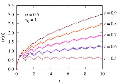
Figure 1: (Color online) Average particle position $\langle x(t)\rangle$ for various values of the parameter $r$ (average force $\bar{F}$) and anomalous exponent $\alpha$. Symbols represent the results from the numerical simulations of the CTRW obtained by averaging over $10^{5}$ trajectories (for $r=0.5$ over $10^{6}$ trajectories). Continuous lines represent the analytical solution (III.1) of the FFPE (6). The time-period of the rectangular force (7) is $\tau_{0}=1$ and the fractional exponent $\alpha=0.5$; in numerical simulations $F_{0}/(\eta_{\alpha}\sqrt{\kappa_{\alpha}})=1$ is used. The value $r=0.9$ corresponds to $\bar{F}=0.8F_{0}$ and $\sigma=0.6F_{0}$; $r=0.8$ corresponds to $\bar{F}=0.6F_{0}$ and $\sigma=0.8F_{0}$; $r=0.7$ corresponds to $\bar{F}=0.4F_{0}$ and $\sigma\approx 0.92F_{0}$; $r=0.6$ corresponds to $\bar{F}=0.2F_{0}$, $\sigma\approx 0.98F_{0}$; and $r=0.5$ to $\bar{F}=0$, $\sigma=F_{0}$.

III Driven subdiffusion

We consider a dichotomous modulation of a biased subdiffusion where the absolute value of the bias is fixed but its direction flips periodically in time, i.e.

$$F(t)=F_{0}\xi(t)$$ (7)

with

$$\xi(t)=\left\{\begin{array}[]{ll}+1&\textrm{~{}for}~{}~{}n\tau_{0}<t<(n+r)\tau_{0}\\ -1&\textrm{~{}for}~{}~{}(n+r)\tau_{0}<t<(n+1)\tau_{0}\end{array}\right..$$ (10)

Here $\tau_{0}$ is the period of the time-dependent force and $n=0,1,2\ldots$ The quantity $r\in(0,1)$ determines the value of the average force:

$$\bar{F}=\langle F(t)\rangle_{\tau_{0}}=F_{0}(2r-1)\,.$$ (11)

For $r=0.5$ the average bias is zero and we recover the model investigated in Ref. heinsalu2007b . Notice that the force $F(t)$ can be decomposed in the following way: $F(t)=\bar{F}+\tilde{F}(t)$. The asymmetric driving,

$$\tilde{F}(t)\!=\!\left\{\!\begin{array}[]{ll}2F_{0}(1-r)&\textrm{~{}for}~{}~{}n\tau_{0}<t<(n+r)\tau_{0}\\ -2F_{0}r&\textrm{~{}for}~{}~{}(n+r)\tau_{0}<t<(n+1)\tau_{0}\end{array}\right.\!,$$ (14)

has a zero mean value, $\langle\tilde{F}(t)\rangle_{\tau_{0}}=0$, and the driving root-mean-squared (rms) amplitude is $\sigma=\langle\tilde{F}^{2}(t)\rangle^{1/2}_{\tau_{0}}=2F_{0}\sqrt{r(1-r)}$. For a fixed average bias $\bar{F}$, this yields

$$\sigma=2\bar{F}\frac{\sqrt{r(1-r)}}{2r-1}$$ (15)

and therefore one can vary the ratio $\sigma/\bar{F}$ between $0$ for $r=1$ and $\infty$ for $r=1/2+\epsilon$, $\epsilon\to 0$. This offers the way to study the influence of an asymmetric, zero-mean driving $\tilde{F}(t)$ with period $\tau_{0}$ and rms amplitude $\sigma$ on the subdiffusion under constant bias $\bar{F}$.

Let us begin by finding the recurrence relation for the moments $\langle x^{n}(t)\rangle$. Assuming in Eq. (6) the force of the form (7) with (10), multiplying both sides of Eq. (6) by $x^{n}$, and integrating over the $x$-coordinate one obtains,

$$\frac{d\langle x^{n}(t)\rangle}{dt} = nv_{\alpha}\xi(t)\sideset{{}_{0}}{{}_{t}}{\mathop{\hat{D}}^{1-\alpha}}\langle x^{n-1}(t)\rangle$$ (16)

$$+ n(n-1)\kappa_{\alpha}\sideset{{}_{0}}{{}_{t}}{\mathop{\hat{D}}^{1-\alpha}}\langle x^{n-2}(t)\rangle\,,$$

with subvelocity $v_{\alpha}=F_{0}/\eta_{\alpha}$ ($n>1$). For $n=1$ the last term on the right hand side of Eq. (16) is absent,

$$\frac{d\langle x(t)\rangle}{dt}=\frac{v_{\alpha}}{\Gamma(\alpha)}\,\xi(t)\,t^{\alpha-1}\,.$$ (17)

Equations (16) and (17) will be used to calculate the average particle position and the mean square displacement.

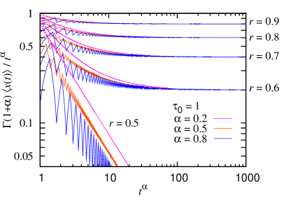
Figure 2: (Color online) The analytical solution (III.1) for average particle position $\langle x(t)\rangle$ obtained from the FFPE (6) is presented for various values of the parameter $r$ (average bias $\bar{F}$) and anomalous exponent $\alpha$. The time-period of the force is $\tau_{0}=1$, however, in the long time limit the same asymptotic value is obtained for any value of $\tau_{0}$. The relation between $r$ and $\bar{F}$ and $\sigma$ is the same as in Fig. 1.

III.1 Average particle position

Upon integrating Eq. (17) in time with $\xi(t)$ given by (10), the solution for the average particle position reads:

$$\langle x(t)\rangle$$

$$=\left\{\begin{array}[]{l@{\quad\quad}}x_{N}+\frac{v_{\alpha}t^{\alpha}}{\Gamma(\alpha+1)}\,,\quad N\tau_{0}\leq t<(N+r)\tau_{0}\\ x_{N}^{\prime}-\frac{v_{\alpha}t^{\alpha}}{\Gamma(\alpha+1)}\,,\quad(N+r)\tau_{0}\leq t<(N+1)\tau_{0}\end{array}\right.$$ (20)

with

$$x_{N} = \langle x(0)\rangle-\frac{v_{\alpha}(N\tau_{0})^{\alpha}}{\Gamma(\alpha+1)}+\frac{v_{\alpha}\tau_{0}^{\alpha}}{\Gamma(\alpha+1)}$$ (21)

$$\times \sum_{n=0}^{N-1}\left[2(n+r)^{\alpha}-n^{\alpha}-(n+1)^{\alpha}\right]\,,$$

$$x_{N}^{\prime} = x_{N}+\frac{2v_{\alpha}\tau_{0}^{\alpha}}{\Gamma(\alpha+1)}(N+r)^{\alpha}\,;$$ (22)

$N$ counts the number of time periods passed.

When the average bias is zero, i.e., $r=0.5$, in the long time limit the mean particle position approaches the constant value

$$\langle x(\infty)\rangle=v_{\alpha}\tau_{0}^{\alpha}b(\alpha)/\Gamma(\alpha+1),$$ (23)

with $b(\alpha)=\sum_{n=0}^{\infty}[2(n+1/2)^{\alpha}-n^{\alpha}-(n+1)^{\alpha}]$. The function $b(\alpha)$ changes monotonously from $b(0)=1$ to $b(1)=0$. It describes the initial field phase effect which the system remembers forever when $\alpha\in(0,1)$ (see also Ref. heinsalu2007b ). This is one of the main differences between the anomalous motion in the absence of a force and in the presence of a time-dependent field with zero average value.

In Fig. 1 the analytical solution (III.1) for the mean particle position $\langle x(t)\rangle$, obtained from the FFPE (6), is compared with the numerical solution of the CTRW for different values of $r$, i.e. for different values of the average bias $\bar{F}$. In Fig. 2 the solution (III.1) is presented in the long time limit for various values of $r$ and $\alpha$. Figures 1 and 2 demonstrate that in the presence of an average bias the mean particle position grows as $t^{\alpha}$. For all values of $r$, the asymptotic value of subvelocity corresponds to the averaged bias $\bar{F}=F_{0}(2r-1)$, indicating that the periodic unbiased field does not affect the subdiffusion current for different values $\bar{F}$ and the field rms-amplitude $\sigma$.

Furthermore, the results depicted in Figs. 1 and 2 clearly show the phenomenon of the “death of linear response” of the fractional kinetics to time-dependent fields in the limit $t\to\infty$: the amplitude of the oscillations decays to zero as $1/t^{1-\alpha}$, Eq. (17) (see also Refs. Barbi ; SokolovKlafter06 ). The amplitude of the oscillations is larger for larger values of $\alpha$ and of $\tau_{0}$. However, $\Gamma(1+\alpha)\langle x(t)\rangle/t^{\alpha}$ reaches asymptotically the same value for any $\alpha$ and $\tau_{0}$.

III.2 Mean square displacement

Let us now study the mean square displacement, defined as

$$\langle\delta x^{2}(t)\rangle=\langle x^{2}(t)\rangle-\langle x(t)\rangle^{2}\,.$$ (24)

For $n=2$ one obtains from Eq. (16),

$$\frac{d\langle x^{2}(t)\rangle}{dt}=2v_{\alpha}\xi(t)\sideset{{}_{0}}{{}_{t}}{\mathop{\hat{D}}^{1-\alpha}}\langle x(t)\rangle+\frac{2\kappa_{\alpha}}{\Gamma(\alpha)}\,t^{\alpha-1}\,.$$ (25)

In order to find the analytical solution for the mean square displacement, we use the Laplace-transform method and the Fourier series expansion for $\xi(t)=\xi(t+\tau_{0})$ given wuth Eq. (10),

$$\xi(t)=\sum_{n=-\infty}^{\infty}f_{n}\exp(in\omega_{0}t)\,,$$ (26)

with

$$f_{n} = \frac{1}{\tau_{0}}\int_{0}^{\tau_{0}}\xi(t)\exp(-in\omega_{0}t)dt$$ (27)

$$= [1-\exp(-inr2\pi)]/(in\pi)$$

and $\omega_{0}=2\pi/\tau_{0}$. Applying them to Eq. (25) and assuming $\langle x(0)\rangle=0$ and $\langle x^{2}(0)\rangle=0$ we obtain that in the long time limit (see Appendix A),

$$\langle x^{2}(t)\rangle = \frac{2v_{\alpha}^{2}(2r-1)^{2}}{\Gamma(2\alpha+1)}t^{2\alpha}+\frac{2\kappa_{\alpha}}{\Gamma(\alpha+1)}t^{\alpha}$$ (28)

$$+ \frac{2v_{\alpha}^{2}(2r-1)S_{1}}{\omega_{0}^{\alpha}\Gamma(\alpha+1)}t^{\alpha}+\frac{8v_{\alpha}^{2}\cos(\alpha\pi/2)}{\pi^{2}\omega_{0}^{\alpha}\Gamma(\alpha+1)}$$

$$\times \left[\zeta(2+\alpha)-\sum_{n=1}^{\infty}\frac{\cos(nr2\pi)}{n^{2+\alpha}}\right]t^{\alpha}\,;$$

here $\zeta(x)$ is the Riemann’s zeta-function and $S_{1}$ is a function of $\alpha$ and $r$ as given by Eq. (A) in Appendix A.

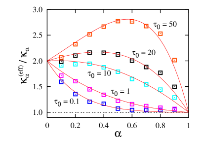
Figure 3: (Color online) Scaled effective fractional diffusion coefficient $\kappa_{\alpha}^{\mathrm{(eff)}}$ versus fractional exponent $\alpha$ for different driving periods $\tau_{0}$. The average bias is zero ($r=0.5$). The analytical prediction (29) (continuous lines) is compared with the results (symbols) obtained from the numerical simulation of the CTRW by averaging over $10^{5}$ trajectories. For $\tau_{0}>\tau_{0}^{*}\approx 8.818$ heinsalu2007b the effective fractional diffusion coefficient $\kappa_{\alpha}^{\mathrm{(eff)}}(\alpha)$ exhibits a maximum.

For $r=0.5$ (average zero bias) the first and third term in Eq. (28) are equal to zero. Furthermore, in the long time limit the average particle position $\langle x(\infty)\rangle$ is a finite constant. The asymptotic behavior of the mean square displacement is thus proportional to $t^{\alpha}$ as in the force free case, however, characterized by an effective fractional diffusion coefficient $\kappa_{\alpha}^{\mathrm{(eff)}}$ instead of the free fractional diffusion coefficient $\kappa_{\alpha}$, i.e. $\langle\delta x^{2}(t)\rangle=2\kappa_{\alpha}^{\mathrm{(eff)}}t^{\alpha}/\Gamma(1+\alpha)$ for $t\to\infty$. The effective diffusion coefficient is heinsalu2007b ,

$$\kappa_{\alpha}^{\mathrm{(eff)}} = \kappa_{\alpha}+\frac{8F_{0}^{2}}{\pi^{2}\eta_{\alpha}^{2}\omega_{0}^{\alpha}}\,\zeta(\alpha+2)$$ (29)

$$\times \left(1-\frac{1}{2^{\alpha+2}}\right)\cos(\alpha\pi/2)\,.$$

The driving-induced part of the effective subdiffusion coefficient is directly proportional to the square of driving amplitude $F_{0}$ and inversely proportional to $\omega_{0}^{\alpha}$. For slowly oscillating force fields this leads to a profound acceleration of subdiffusion compared with the force free case: an optimal value of the fractional exponent $\alpha$ exists, at which the driving-induced part of the effective fractional diffusion coefficient possesses a maximum (see Fig. 3).

When $r\neq 0.5$ (finite average force) we obtain in the long time limit for $\langle x(t)\rangle^{2}$ (see Appendix B),

$$\langle x(t)\rangle^{2}=\frac{v_{\alpha}^{2}(2r-1)^{2}}{\Gamma^{2}(\alpha+1)}t^{2\alpha}+\frac{2v_{\alpha}^{2}(2r-1)S_{1}}{\omega_{0}^{\alpha}\Gamma(\alpha+1)}t^{\alpha}$$ (30)

[$S_{1}$ is given by Eq. (A) in Appendix A]. Clearly, the leading term in Eq. (30) corresponds to subvelocity in constant field $\bar{F}$ (averaged bias), i.e. the influence of periodic, unbiased driving $\tilde{F}(t)$ dies asymptotically out, as illustrated in Fig. 2.

The results (28) and (30) indicate that in the presence of a rectangular time-periodic force with a finite average value the general behavior of the mean square displacement is similar to the case of a constant force, i.e. the mean square displacement $\langle\delta x^{2}(t)\rangle$ consists of terms proportional to $t^{\alpha}$ and $t^{2\alpha}$. In fact, for the leading term proportional to $t^{2\alpha}$ in the mean square displacement one obtains the coefficient

$$\frac{{\bar{F}}^{2}}{\eta_{\alpha}^{2}}\left[\frac{2}{\Gamma(2\alpha+1)}-\frac{1}{\Gamma^{2}(\alpha+1)}\right]\,.$$

This coefficient is the same as in the case of the subdiffusive motion under the influence of a constant force if the value of the constant force would be $\bar{F}$.

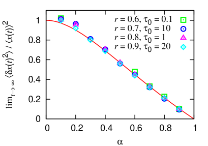
Figure 4: (Color online) The asymptotic scaling relation (31). Symbols correspond to the numerical results obtained from the CTRW for different values of $r$ ($r\neq 0.5$) and $\tau_{0}$. Solid curve corresponds to the analytical result (31). Different values of the parameter $r$ correspond to different values of the bias $\bar{F}$ and the periodic field rms $\sigma$, as described in Fig. 1. The field parameters do not influence the results within the statistical errors.

Furthermore, similarly to the case of a constant bias, the asymptotic scaling relation holds ($r\neq 0.5$, $\bar{F}\neq 0$) between the mean square displacement and average particle position. In the limit $t\to\infty$ the mean square displacement grows as $\langle\delta x^{2}(t)\rangle\propto t^{2\alpha}$ and

$$\lim_{t\to\infty}\frac{\langle\delta x^{2}(t)\rangle}{\langle x(t)\rangle^{2}}=\frac{2\Gamma^{2}(\alpha+1)}{\Gamma(2\alpha+1)}-1\,,\quad\bar{F}\neq 0\,.$$ (31)

It is illustrated by Fig. 4, where the analytical curve [Eq. (31)] is compared with the numerical results. The universality of relation (31) under the unbiased driving $\tilde{F}(t)$ means that the biased diffusion is not affected by the driving. This is in a sharp contrast with the unbiased diffusion in Fig. 3.

IV Conclusion

With this work we presented the derivation of the FFPE (6) for a special class of space- and time-dependent force fields from the underlying CTRW picture. Our derivation shows along with the corresponding discussion that it is difficult to justify this equation for time-dependent forces different from $F(x,t)=F(x)\xi(t)$ with $\xi(t)=\pm 1$ beyond the linear response approximation. Using the FFPE (6) we demonstrated that the universal scaling relation (31) for a biased subdiffusion is not affected by the additional action of a time-periodic zero-mean rectangular driving; neither is the asymptotic anomalous current nor the anomalous biased diffusion. We argue that this result is general and it is valid for other driving forms as well. This driving-immunity is due to the fact that the CTRW subdiffusion occurs in a random operational time which lacks mean value, whereas any physical field changes in the real, physical time. The CTRW-based subdiffusion fails to respond asymptotically to such time-dependent fields while on its intrinsic random operational time scale any real, alternating field is acting infinitely fast and it makes effectively no influence in a long run heinsalu2007b ; goychuk07 , unless the rate of its change is precisely zero. This is the main reason for the observed anomalies. The remarkable enhancement of the unbiased subdiffusion within the CTRW framework by time-periodic rectangular fields is rather an exception than the rule.

Appendix A

Using the property $\mathcal{L}\{df(t)/dt\}=s\mathcal{L}\{f(t)\}-f(0)$ and assuming the initial conditions $\langle x(t)\rangle=0$ and $\langle x^{2}(t)\rangle=0$ we obtain from Eq. (25),

$$\mathcal{L}\{\langle x^{2}(t)\rangle\}=\frac{2\kappa_{\alpha}}{s^{\alpha+1}}+\frac{2v_{\alpha}}{s}\mathcal{L}\{\xi(t)\sideset{{}_{0}}{{}_{t}}{\mathop{\hat{D}}^{1-\alpha}}\langle x(t)\rangle\}\,.$$ (32)

Considering that

$$\mathcal{L}\{\sideset{{}_{0}}{{}_{t}}{\mathop{\hat{D}}^{1-\alpha}}\langle x(t)\rangle\}=s^{1-\alpha}\mathcal{L}\{\langle x(t)\rangle\}=s^{-\alpha}\mathcal{L}\{d\langle x(t)\rangle/dt\}\,,$$

one obtains,

$$\mathcal{L}\{\xi(t)\sideset{{}_{0}}{{}_{t}}{\mathop{\hat{D}}^{1-\alpha}}\langle x(t)\rangle\} = \sum_{n=-\infty}^{\infty}\frac{f_{n}}{(s-in\omega_{0})^{\alpha}}$$ (33)

$$\times \mathcal{L}_{s-in\omega_{0}}\left\{\frac{d\langle x(t)\rangle}{dt}\right\}\,.$$

Using Eq. (17) with (26), it follows,

$$\mathcal{L}_{s-in\omega_{0}}\left\{\frac{d\langle x(t)\rangle}{dt}\right\}=v_{\alpha}\sum_{m=-\infty}^{\infty}\frac{f_{m}}{[s-i\omega_{0}(n+m)]^{\alpha}}\,.$$ (34)

Inserting (33) and (34) into Eq. (32) we obtain,

$$\mathcal{L}\{\langle x^{2}(t)\rangle\} = \frac{2\kappa_{\alpha}}{s^{\alpha+1}}+\frac{2v_{\alpha}^{2}}{s}\sum_{n=-\infty}^{\infty}\frac{f_{n}}{(s-in\omega_{0})^{\alpha}}$$ (35)

$$\times \sum_{m=-\infty}^{\infty}\frac{f_{m}}{[s-i\omega_{0}(n+m)]^{\alpha}}\,.$$

Let us separate in Eq. (35) the terms $m=0$ and $n=0$,

$$\mathcal{L} \{\langle x^{2}(t)\rangle\}=\frac{2\kappa_{\alpha}}{s^{\alpha+1}}+\frac{2v_{\alpha}^{2}f_{0}^{2}}{s^{2\alpha+1}}$$ (36)

$$+ \frac{2v_{\alpha}^{2}f_{0}}{s^{\alpha+1}}\sum_{\begin{subarray}{c}m=-\infty\\ m\neq 0\end{subarray}}^{\infty}\frac{f_{m}}{(s-im\omega_{0})^{\alpha}}+\frac{2v_{\alpha}^{2}}{s}\sum_{\begin{subarray}{c}n=-\infty\\ n\neq 0\end{subarray}}^{\infty}\frac{f_{n}}{(s-in\omega_{0})^{\alpha}}$$

$$\times \sum_{m=-\infty}^{\infty}\frac{f_{m}}{[s-i\omega_{0}(n+m)]^{\alpha}}\,.$$

In the long time limit, i.e., in the limit $s\to 0$, in the double sum only terms with $m=-n$ contribute, giving thus,

$$\mathcal{L}\{\langle x^{2}(t)\rangle\} = \frac{2\kappa_{\alpha}}{s^{\alpha+1}}+\frac{2v_{\alpha}^{2}f_{0}^{2}}{s^{2\alpha+1}}+\frac{2v_{\alpha}^{2}f_{0}}{\omega_{0}^{\alpha}s^{\alpha+1}}\sum_{\begin{subarray}{c}m=-\infty\\ m\neq 0\end{subarray}}^{\infty}\frac{f_{m}}{(-im)^{\alpha}}$$ (37)

$$+ \frac{2v_{\alpha}^{2}}{\omega_{0}^{\alpha}s^{\alpha+1}}\sum_{\begin{subarray}{c}n=-\infty\\ n\neq 0\end{subarray}}^{\infty}\frac{|f_{n}|^{2}}{(-in)^{\alpha}}\,.$$

Let us compute the sums. Considering that

$$\sum_{\begin{subarray}{c}m=-\infty\\ m\neq 0\end{subarray}}^{\infty}\frac{f_{m}}{(-im)^{\alpha}}=\sum_{m=1}^{\infty}\left[\frac{f_{m}}{(-im)^{\alpha}}+\frac{f_{-m}}{(im)^{\alpha}}\right]\,,$$

and replacing here $f_{m}$ from (27), one obtains,

$$\sum_{\begin{subarray}{c}m=-\infty\\ m\neq 0\end{subarray}}^{\infty}\frac{f_{m}}{(-im)^{\alpha}}=\left.\frac{2}{\pi}\right[\zeta(1+\alpha)\sin{(\alpha\pi/2)}$$

$$-\sum_{m=1}^{\infty}\left.\frac{\sin{[(\alpha-4mr)\pi/2]}}{m^{1+\alpha}}\right]\equiv S_{1}\,;$$ (38)

here $\zeta(x)$ is the Riemann’s zeta-function. Analogously,

$$\!\!\!\!\sum_{\begin{subarray}{c}n=-\infty\\ n\neq 0\end{subarray}}^{\infty}\!\frac{|f_{n}|^{2}}{(-in)^{\alpha}}\!\! = \!\!\frac{4}{\pi^{2}}\cos(\alpha\pi/2)$$ (39)

$$\times \!\!\!\left[\zeta(2+\alpha)-\sum_{n=1}^{\infty}\frac{\cos(nr2\pi)}{n^{2+\alpha}}\right]\,.$$

Replacing these sums into Eq. (37) and considering that $f_{0}=2r-1$ [see (27) together with (10)], we get,

$$\mathcal{L}\{\langle x^{2}(t)\rangle\}=\frac{2v_{\alpha}^{2}(2r-1)^{2}}{s^{2\alpha+1}}+\frac{2\kappa_{\alpha}}{s^{\alpha+1}}+\frac{2v_{\alpha}^{2}(2r-1)S_{1}}{\omega_{0}^{\alpha}s^{\alpha+1}}$$

$$+\frac{8v_{\alpha}^{2}}{\pi^{2}\omega_{0}^{\alpha}s^{\alpha+1}}\cos(\alpha\pi/2)\left[\zeta(2+\alpha)-\sum_{n=1}^{\infty}\frac{\cos(nr2\pi)}{n^{2+\alpha}}\right]\,.$$

Taking here the inverse Laplace transform one obtains the expression for $\langle x^{2}(t)\rangle$ in the long time limit [Eq.(28)].

Appendix B

Using Eq. (17), the quantity $\langle x(t)\rangle^{2}$ can be written in the following way,

$$\langle x(t)\rangle^{2}=\frac{2v_{\alpha}^{2}}{\Gamma^{2}(\alpha)}\int_{0}^{t}dt^{\prime}\int_{0}^{t^{\prime}}\xi(t^{\prime})t^{\prime\alpha-1}\xi(t^{\prime\prime})t^{\prime\prime\alpha-1}dt^{\prime\prime}\,.$$ (41)

Exploiting the property $\mathcal{L}\{\int_{0}^{t}f(t^{\prime})dt^{\prime}\}=s^{-1}\mathcal{L}\{f(t^{\prime})\}$ and denoting $t^{\prime}=t$ and $t^{\prime\prime}=t^{\prime}$, we can write,

$$\mathcal{L} \{\langle x(t)\rangle^{2}\}=\frac{2v_{\alpha}^{2}}{\Gamma^{2}(\alpha)s}\mathcal{L}\left\{\xi(t)t^{\alpha-1}\int_{0}^{t}\xi(t^{\prime})t^{\prime\alpha-1}dt^{\prime}\right\}$$ (42)

$$= \frac{2v_{\alpha}^{2}}{\Gamma^{2}(\alpha)s}\sum_{n=-\infty}^{\infty}f_{n}\sum_{m=-\infty}^{\infty}f_{m}$$

$$\times \mathcal{L}_{s-in\omega_{0}}\left\{t^{\alpha-1}\int_{0}^{t}t^{\prime\alpha-1}\exp(im\omega_{0}t^{\prime})dt^{\prime}\right\}\,.$$

For $\alpha=1$ the latter equation gives,

$$\mathcal{L}\{\langle x(t)\rangle^{2}\} = \frac{2v_{\alpha}^{2}}{s}\sum_{n=-\infty}^{\infty}\frac{f_{n}}{s-in\omega_{0}}$$ (43)

$$\times \sum_{m=-\infty}^{\infty}\frac{f_{m}}{s-i\omega_{0}(n+m)}\,.$$

Comparing this result with Eq. (35) we see that $\mathcal{L}\{\langle\delta x^{2}(t)\rangle\}=2\kappa_{\alpha}/s^{2}$, and thus $\langle\delta x^{2}(t)\rangle=2\kappa_{\alpha}t$, as it should be for normal Brownian motion.

For $0<\alpha<1$ it is more convenient to proceed as follows. Let us calculate the Laplace trasform of $\langle x(t)\rangle$. Considering that $\mathcal{L}\{\langle x(t)\rangle\}=s^{-1}\mathcal{L}\{d\langle x(t)\rangle/dt\}$ one obtains [see (34)],

$$\mathcal{L}\{\langle x(t)\rangle\} = v_{\alpha}\sum_{n=-\infty}^{\infty}\frac{f_{n}}{s(s-in\omega_{0})^{\alpha}}$$ (44)

$$= \frac{v_{\alpha}f_{0}}{s^{1+\alpha}}+v_{\alpha}\sum_{\begin{subarray}{c}n=-\infty\\ n\neq 0\end{subarray}}^{\infty}\frac{f_{n}}{s(s-in\omega_{0})^{\alpha}}\,.$$

In the limit $t\to\infty$, i.e. $s\to 0$, the latter equation becomes,

$$\mathcal{L}\{\langle x(t)\rangle\}=\frac{v_{\alpha}f_{0}}{s^{1+\alpha}}+\frac{v_{\alpha}}{s}\sum_{\begin{subarray}{c}n=-\infty\\ n\neq 0\end{subarray}}^{\infty}\frac{f_{n}}{(-in\omega_{0})^{\alpha}}\,.$$ (45)

Taking into account (A) we can write,

$$\mathcal{L}\{\langle x(t)\rangle\}=\frac{v_{\alpha}f_{0}}{s^{1+\alpha}}+\frac{v_{\alpha}S_{1}}{\omega_{0}^{\alpha}s}\,.$$ (46)

Taking here the inverse Laplace transform we have for $t\to\infty$,

$$\langle x(t)\rangle=\frac{v_{\alpha}(2r-1)}{\Gamma(\alpha+1)}\,t^{\alpha}+\frac{v_{\alpha}S_{1}}{\omega_{0}^{\alpha}}\,.$$ (47)

From here one obtains the result (30) for $\langle x(t)\rangle^{2}$.

References

• (1) J. P. Bouchaud and A. Georges, Phys. Rep. 195, 127 (1990).
• (2) H. Scher, M. F. Shlesinger, and J. T. Bendler, Physics Today 44 (1), 26 (1991); M. F. Shlesinger, G. M. Zaslavsky, and J. Klafter, Nature 363, 31 (1993); J. Klafter, M. F. Shlesinger, and G. Zumofen, Physics Today 49 (2), 33 (1996).
• (3) H. Scher and E. W. Montroll, Phys. Rev. B 12, 2455 (1975).
• (4) M. F. Shlesinger, J. Stat. Phys. 10, 421 (1974).
• (5) G. Bel and E. Barkai, Phys. Rev. Lett. 94, 240602 (2005).
• (6) R. Metzler and J. Klafter, Phys. Rep. 339, 1 (2000); R. Metzler, E. Barkai, and J. Klafter, Phys. Rev. Lett. 82, 3563 (1999); E. Barkai, Phys. Rev. E 63, 046118 (2001).
• (7) I. Goychuk, E. Heinsalu, M. Patriarca, G. Schmid, and P. Hänggi, Phys. Rev. E 73, 020101(R) (2006).
• (8) E. Heinsalu, M. Patriarca, I. Goychuk, G. Schmid, and P. Hänggi, Phys. Rev. E 73, 046133 (2006).
• (9) P. Hänggi and H. Thomas, Phys. Rep. 88, 207 (1982).
• (10) H. C. Fogedby, Phys. Rev. E 50, 1657 (1994).
• (11) A. A. Stanislavsky, Phys. Rev. E 67, 021111 (2003).
• (12) M. Magdziarz, A. Weron, and K. Weron, Phys. Rev. E 75, 016708 (2007).
• (13) E. Heinsalu, M. Patriarca, I. Goychuk, and P. Hänggi, Phys. Rev. Lett. 99, 120602 (2007).
• (14) I. Goychuk, Phys. Rev. E 76, 040102(R) (2007).
• (15) I. Goychuk and P. Hänggi, Phys. Rev. E 69, 021104 (2004).
• (16) I. M. Sokolov and J. Klafter, Phys. Rev. Lett. 97, 140602 (2006).
• (17) I. M. Sokolov, A. Blumen, and J. Klafter, Europhys. Lett. 56, 175 (2001); I. M. Sokolov, A. Blumen, and J. Klafter, Physica A 302, 268 (2001).
• (18) See, e.g. in: J.-L. Dejardin and J. Jadzyn, J. Chem. Phys. 123, 174502 (2005); M. Y. Yim and K. L. Liu, Physica A 369, 329 (2006).
• (19) V. M. Kenkre, E. W. Montroll, and M. F. Shlesinger, J. Stat. Phys. 9, 45 (1973); A. I. Burshtein, A. A. Zharikov, and S. I. Temkin, Theor. Math. Phys. 66, 166 (1986); I. Goychuk, Phys. Rev. E 70, 016109 (2004).
• (20) B. D. Hughes, Random Walks and Random Environments, Vol. 1: Random Walks (Clarendon Press, Oxford, 1995).
• (21) G. H. Weiss, Aspects and Applications of the Random Walk (North-Holland, Amsterdam, 1994).
• (22) I. Goychuk, P. Hänggi, J. L. Vega, and S. Miret-Artes, Phys. Rev. E 71, 061906 (2005).
• (23) F. Barbi, M. Bologna, and P. Grigolini, Phys. Rev. Lett. 95, 220601 (2005).