CASIMIR FORCE ON AMPLIFYING BODIES

Abstract

Based on a unified approach to macroscopic QED that allows for the inclusion of amplification in a limited space and frequency range, we study the Casimir force as a Lorentz force on an arbitrary partially amplifying system of linearly locally responding (isotropic) magnetoelectric bodies. We demonstrate that the force on a weakly polarisable/magnetisable amplifying object in the presence of a purely absorbing environment can be expressed as a sum over the Casimir–Polder forces on the excited atoms inside the body. As an example, the resonant force between a plate consisting of a dilute gas of excited atoms and a perfect mirror is calculated.

I Introduction

Improved measurement methods Lamoreaux (2005) and the possibility of fabricating metamaterials Rockstuhl et al. (2007); Liu et al. (2008); Yang and Li (2008) and in particular, lefthanded materials (e.g. Refs. Smith et al. (2000); Shelby et al. (2001); Lezec et al. (2007); Paul et al. (2008)), have motivated a number of recent investigations into dispersion forces on micro- and macro-objects with specially tailored magnetoelectric properties. In this context, dispersion forces on ground-state systems such as the Casimir–Polder (CP) interaction between a ground-state atom and a magnetoelectric body Buhmann et al. (2005) and the van der Waals (vdW) interaction between two ground-state atoms in a magneto-electric medium Spagnolo et al. (2007) have been studied. In both cases it was found lefthanded medium properties, being realised in certain finite frequency windows, are unable to noticeably affect these ground-state forces which depend on the medium response at all frequencies in an integral form. In the same spirit, the Casimir force between macroscopic bodies with metamaterial properties has been studied where possible anisotropy Rosa et al. (2008) and lefthandedness Yang et al. (2008) has been taken into account. It could again be shown that the strength and the sign of the dispersion force is influenced by the strength of the magnetic properties rather than the lefthandedness Henkel and Joulain (2005); Tomaš (2005a).

To enhance the impact of a lefthanded magnetoelectric response, it is natural to consider the resonant force components acting on excited systems, which depend on single selected frequencies. The vdW interaction has initially been studied for atoms in free space for the cases of one ground-state and one excited atom Power and Thirunamachandran (1995a); Rizzuto et al. (2004); Sherkunov (2005), two excited atoms Power and Thirunamachandran (1995a) and three atoms with one of them being excited Power and Thirunamachandran (1995b); Passante et al. (2005). The presence of ground-state media was taken into account in Ref. Sherkunov (2007a). Similarly, the resonant CP interaction of a macroscopic ground-state body and an excited atom has been studied Wylie and Sipe (1984); Buhmann et al. (2004a); Sherkunov (2007b). Applying the general results to a geometry involving a lefthanded slab, it was noted that the inclusion of material absorption is crucial when studying CP forces on excited atoms Sambale et al. (2008a, b). Measurements of the CP energy of excited atoms are typically based on spectroscopic methods Sandoghdar et al. (1992); Chevrollier et al. (2001); Failache et al. (2003).

Excitations can also be present in the electromagnetic field, with thermal fields being an important special case. The impact of thermal fields on the Casimir force has been subject to discussions Ninham and Daicic (1998); Mostepanenko et al. (2006) and experiments Decca et al. (2005); Klimchitskaya et al. (2005). While the Casimir force and the CP force McLachlan (1963); Henkel et al. (2002); Gorza and Ducloy (2006) at thermal equilibrium are nonresonant, integral effects just like their zero-temperature counterparts, interesting phenomena can particularly arise for nonequilibrium systems. For instance, the CP force on an atom near a body held at a temperature different from that of the environment can be attractive or repulsive depending on the temperature difference Antezza et al. (2005), as has been confirmed experimentally Harber et al. (2005); Obrecht et al. (2007). It has further been shown that even a ground-state atom can be subject to resonant force components when placed in a finite-temperature environment Buhmann and Scheel (2008a). The vdW interaction between two atoms has recently even been studied in the presence of more general electromagnetic fields Sherkunov (2008).

Although excitation has thus been included in the theories in various forms, dispersion forces on or in the presence of amplifying media have not been in focus yet, although such materials are indispensable in laser physics Scully and Zubairy (1997) and have recently attracted interest in the context of metamaterials Popov and Shalaev (2006); Stockmann (2007). In particular, they are proposed to lead to repulsive forces Leonhardt and Philbin (2007) and may therefore be used to overcome the problem of stiction Zhao (2003). As has been pointed out by various authors Rosa et al. (2008); Raabe and Welsch (2008), the analysis leading to this prediction lacks a rigorous treatment of amplification. A microscopic approach to the problem was developed in Ref. Sherkunov (2005) where the CP potential of a ground-state atom in front of an excited dilute gaseous medium, as well as the Casimir interaction between two dilute samples of excited gas atoms has been calculated. To go beyond such dilute-gas limits, an inclusion of amplification in the quantisation scheme is necessary. To our knowledge, the first attempt in this direction has been made in Ref. Jeffers et al. (1996); Matloob et al. (1997) where the light propagates perpendicular to a dielectric amplifying slab. Within the framework of macroscopic QED, a full picture of the quantisation of the medium-assisted electromagnetic field in the presence of arbitrary (absorbing or amplifying) linear, causal media has been developed very recently Raabe and Welsch (2008). This formalism is used in the present work to develop a consistent theory of the Casimir force on a body made of an amplifying metamaterial which generalises microscopic results beyond the dilute-gas limit.

The paper is organised as follows. In Sec. II we show how the quantisation scheme of medium-assisted electromagnetic field should be extended in the presence of body that is amplifying in a certain space- and frequency regime. After calculating the Casimir force on an arbitrary amplifying body in Sec. III, we make contact to the microscopic CP forces on the excited atoms contained inside this body (Sec. IV). As an example, we consider the Casimir force on a dilute slab of excited gas atoms. The paper ends with the summary in Sec. VI.

II Macroscopic quantum electrodynamics for amplifying media

We consider an arrangement of linear, local (isotropic) magnetoelectric bodies some of which are (linearly) amplifying in a limited frequency range and absorbing in the remaining frequency range. The bodies are described by spatially varying complex electric permittivity $\varepsilon({\bf r},\omega)$ and $\mu({\bf r},\omega)$ that fulfil the Kramers–Kronig relations. The electric or magnetic response of the bodies is amplifying if ${\rm Im}\,\varepsilon({\bf r},\omega)=\varepsilon_{I}({\bf r},\omega)<0$ or ${\rm Im}\,\mu({\bf r},\omega)=\mu_{I}({\bf r},\omega)<0$ hold, respectively. Note that the strength of the amplification should be chosen such that the response to electromagnetic field is still linear. In particular we assume that the medium-assisted field is in an excited state where the medium is pumped in such a way that the state of the field can be regarded as quasi-stationary (for details, Raabe and Welsch (2008)).

The quantised electric field in the presence of the partially amplifying media can be given as the solution to the familiar Helmholtz equation

$$\biggl{[}\bm{\nabla}\times\frac{1}{\mu({\bf r},\omega)}\bm{\nabla}\times-\frac{\omega^{2}}{c^{2}}\varepsilon({\bf r},\omega)\biggr{]}\hat{\underline{{\bf E}}}({\bf r},\omega)=i\mu_{0}\omega\hat{\underline{{\bf j}}}_{N}({\bf r},\omega)$$ (1)

according to

$$\hat{\underline{{\bf E}}}({\bf r},\omega)=i\omega\mu_{0}\int\mathrm{d}^{3}r^{\prime}\mbox{{{G}}}({\bf r},{\bf r^{\prime}},\omega)\cdot\hat{\underline{{\bf j}}}_{N}({\bf r^{\prime}},\omega)$$ (2)

where the classical Green tensor obeys the differential equation

$$\biggl{[}\bm{\nabla}\times\frac{1}{\mu({\bf r},\omega)}\bm{\nabla}\times-\frac{\omega^{2}}{c^{2}}\varepsilon({\bf r},\omega)\biggr{]}\mbox{{{G}}}({\bf r},{\bf r^{\prime}},\omega)=\bm{\delta}({\bf r}-{\bf r^{\prime}})$$ (3)

together with the boundary condition at infinity. This differential equation can be cast into its equivalent form

$$\biggl{(}\bm{\nabla}\times\bm{\nabla}\times-\frac{\omega^{2}}{c^{2}}\biggr{)}\mbox{{{G}}}({\bf r},{\bf r}^{\prime},\omega)$$

$$=\bm{\delta}({\bf r}-{\bf r}^{\prime})+\frac{\omega^{2}}{c^{2}}[\varepsilon({\bf r},\omega)-1]\mbox{{{G}}}({\bf r},{\bf r^{\prime}},\omega)$$

$$\quad+\bm{\nabla}\times\biggl{[}1-\frac{1}{\mu({\bf r},\omega)}\biggr{]}\bm{\nabla}\times\mbox{{{G}}}({\bf r},{\bf r^{\prime}},\omega)$$

$$=\bm{\delta}({\bf r}-{\bf r}^{\prime})+i\mu_{0}\omega\int\mathrm{d}^{3}s\mbox{{{Q}}}({\bf r},{\bf s},\omega)\cdot\mbox{{{G}}}({\bf s},{\bf r}^{\prime},\omega)$$ (4)

by introducing the conductivity tensor Kubo et al. (1998); Melrose and McPhedran (2003)

$$\mbox{{{Q}}}({\bf r},{\bf r^{\prime}},\omega)=\sum_{\lambda=e,m}\mbox{{{Q}}}_{\lambda}({\bf r},{\bf r^{\prime}},\omega),$$ (5)

$$\mbox{{{Q}}}_{e}({\bf r},{\bf r^{\prime}},\omega)=-i\varepsilon_{0}\omega[\varepsilon({\bf r},\omega)-1]\bm{\delta}({\bf r}-{\bf r^{\prime}}),$$ (6)

$$\mbox{{{Q}}}_{m}({\bf r},{\bf r^{\prime}},\omega)=-\frac{1}{i\omega\mu_{0}}\bm{\nabla}\!\times\!\biggl{[}1\!-\!\frac{1}{\mu({\bf r},\omega)}\biggr{]}\!\bm{\delta}({\bf r}\!-\!{\bf r^{\prime}})\!\times\!\overleftarrow{\bm{\nabla}}^{\prime}.$$ (7)

It is well known that in the presence of amplification the roles of the noise creation and noise destruction operators are to be exchanged Scheel et al. (1998). Hence, the noise current density reads

$$\hat{\underline{{\bf j}}}_{N}({\bf r},\omega)=\omega\sqrt{\frac{\hbar\varepsilon_{0}}{\pi}|\varepsilon_{I}({\bf r},\omega)|}\\ \times[\Theta[\varepsilon_{I}({\bf r},\omega)]\hat{{\bf f}}_{e}({\bf r},\omega)+\Theta[-\varepsilon_{I}({\bf r},\omega)]\hat{{\bf f}}^{\dagger}_{e}({\bf r},\omega)]\\ +\bm{\nabla}\times\sqrt{\frac{\hbar}{\pi\mu_{0}}\frac{|\mu_{I}({\bf r},\omega)|}{|\mu({\bf r},\omega)|^{2}}}\\ \times[\Theta[\mu_{I}({\bf r},\omega)]\hat{{\bf f}}_{m}({\bf r},\omega)+\Theta[-\mu_{I}({\bf r},\omega)]\hat{{\bf f}}^{\dagger}_{m}({\bf r},\omega)]$$ (8)

[$\Theta$: Theta function, $\Theta(0)\equiv 1$] where the bosonic dynamical variables $\hat{{\bf f}}_{\lambda}({\bf r},\omega)$ [$\lambda=e,m$] have been introduced. They obey the commutation relations

$$\bigl{[}\hat{f}_{\lambda i}({\bf r},\omega),\hat{f}_{\lambda^{\prime}j}({\bf r^{\prime}},\omega^{\prime})\bigr{]}=0=\bigl{[}\hat{f}^{\dagger}_{\lambda i}({\bf r},\omega),\hat{f}^{\dagger}_{\lambda^{\prime}j}({\bf r^{\prime}},\omega^{\prime})\bigr{]}\\ \bigl{[}\hat{f}_{\lambda i}({\bf r},\omega),\hat{f}^{\dagger}_{\lambda^{\prime}j}({\bf r^{\prime}},\omega^{\prime})\bigr{]}=\delta_{\lambda\lambda^{\prime}}\delta_{ij}\delta({\bf r}-{\bf r^{\prime}})\delta(\omega-\omega^{\prime}),$$ (9)

such that the fundamental equal-time commutation relation characteristic for the electromagnetic field holds,

$$[\hat{{\bf E}}({\bf r}),\hat{{\bf B}}({\bf r^{\prime}})]=i\hbar\varepsilon_{0}^{-1}\bm{\nabla}\times\bm{\delta}({\bf r}-{\bf r^{\prime}}),$$ (10)

where the electric and induction fields are given by Eq. (2) and

$$\hat{\underline{{\bf B}}}({\bf r},\omega)=\mu_{0}\int\mathrm{d}^{3}r^{\prime}\bm{\nabla}\times\mbox{{{G}}}({\bf r},{\bf r^{\prime}},\omega)\cdot\hat{\underline{{\bf j}}}_{N}({\bf r^{\prime}},\omega)$$ (11)

[$\hat{\bf O}({\bf r})=\int_{0}^{\infty}\mathrm{d}\omega\hat{\underline{\bf{O}}}({\bf r},\omega)+\rm{H.c.}$], respectively. The vacuum state $|\bigl{\{}0\bigr{\}}\rangle$ of the body-assisted electromagnetic field, i.e., a quasi-stationary equilibrium excited state as introduced in the beginning of this section, is defined by

$$\hat{{\bf f}}_{\lambda}({\bf r},\omega)|\left\{0\right\}\rangle=\bm{0}\quad\forall\lambda,{\bf r},\omega.$$ (12)

From the quantisation procedure it follows that the Hamiltonian of the electromagnetic field

$$\hat{H}=\sum_{\lambda=e,m}\int\mathrm{d}^{3}r\int_{0}^{\infty}\!\!\!\mathrm{d}\omega\,\hbar\omega\>{\rm sgn}[\kappa_{\lambda}({\bf r},\omega)]\hat{{\bf f}}^{\dagger}_{\lambda}({\bf r},\omega)\!\cdot\!\hat{{\bf f}}_{\lambda}({\bf r},\omega)$$ (13)

[$\kappa_{e}=\varepsilon_{I},\kappa_{m}=\mu_{I}$] generates the correct Maxwell equations by means of the Heisenberg equations of motion.

III Casimir force on an amplifying body

In this section, we calculate the Casimir force on a partially amplifying body of volume $V$ in the presence of other bodies outside $V$. It can be identified as the average Lorentz force Raabe and Welsch (2006)

$${\bf F}=\int_{V}\mathrm{d}^{3}r\int_{0}^{\infty}\langle\hat{\rho}({\bf r})\hat{{\bf E}}({\bf r^{\prime}})+\hat{{\bf j}}({\bf r})\times\hat{{\bf B}}({\bf r^{\prime}})\rangle_{{\bf r^{\prime}}\to{\bf r}}$$ (14)

where the fields are given by Eqs. (2) and (11) and the internal charge and current densities read

$$\underline{\hat{\rho}}({\bf r},\omega)=\frac{i\omega}{c^{2}}\bm{\nabla}\cdot\int\mathrm{d}^{3}r^{\prime}\mbox{{{G}}}({\bf r},{\bf r^{\prime}},\omega)\cdot\underline{\hat{{\bf j}}}_{N}({\bf r^{\prime}},\omega),$$ (15)

$$\underline{\hat{{\bf j}}}({\bf r},\omega)=\biggl{(}\bm{\nabla}\times\bm{\nabla}\times-\frac{\omega^{2}}{c^{2}}\biggr{)}\int\mathrm{d}^{3}r^{\prime}\mbox{{{G}}}({\bf r},{\bf r^{\prime}},\omega)\cdot\underline{\hat{{\bf j}}}_{N}({\bf r^{\prime}},\omega).$$ (16)

Note that the coincidence limit ${\bf r^{\prime}}\to{\bf r}$ has to be performed in such a way that (divergent) self forces are discarded.

On using Eq. (8), the commutation relations (9) and Eq. (12), one can easily verify

$$\langle\underline{\hat{{\bf j}}}_{N}({\bf r},\omega)\underline{\hat{{\bf j}}}_{N}({\bf r^{\prime}},\omega^{\prime})\rangle=\mbox{{{0}}}=\langle\underline{\hat{{\bf j}}}^{\dagger}_{N}({\bf r},\omega)\underline{\hat{{\bf j}}}^{\dagger}_{N}({\bf r^{\prime}},\omega^{\prime})\rangle,$$ (17)

$$\langle\underline{\hat{{\bf j}}}_{N}({\bf r},\omega)\underline{\hat{{\bf j}}}^{\dagger}_{N}({\bf r^{\prime}},\omega^{\prime})\rangle$$

$$=\frac{\hbar\omega}{\pi}\delta(\omega-\omega^{\prime})\!\!\sum_{\lambda=e,m}\!\!{\rm Re}\,\mbox{{{Q}}}_{\lambda}(\mathbf{r},\mathbf{r^{\prime}},\omega)\Theta[\kappa_{\lambda}(\mathbf{r},\omega)],$$ (18)

$$\langle\underline{\hat{{\bf j}}}_{N}^{\dagger}({\bf r},\omega)\underline{\hat{{\bf j}}}_{N}({\bf r^{\prime}},\omega^{\prime})\rangle$$

$$=-\frac{\hbar\omega}{\pi}\delta(\omega-\omega^{\prime})\!\!\sum_{\lambda=e,m}\!\!{\rm Re}\,\mbox{{{Q}}}_{\lambda}(\mathbf{r},\mathbf{r^{\prime}},\omega)\Theta[-\kappa_{\lambda}(\mathbf{r},\omega)]$$ (19)

for the vacuum-state expectation values. Combining these results with the definitions (2), (11), (15) and (16), one finds

$$\langle\underline{\hat{\rho}}({\bf r},\omega)\underline{\hat{{\bf E}}}({\bf r^{\prime}},\omega^{\prime})\rangle=\bm{0}=\langle\underline{\hat{\rho}}^{\dagger}({\bf r},\omega)\underline{\hat{{\bf E}}}^{\dagger}({\bf r^{\prime}},\omega^{\prime})\rangle,$$ (20)

$$\langle\underline{\hat{\rho}}({\bf r},\omega)\underline{\hat{{\bf E}}}^{\dagger}({\bf r^{\prime}},\omega^{\prime})\rangle$$

$$=\frac{\hbar}{\pi}\frac{\omega^{2}}{c^{2}}\delta(\omega-\omega^{\prime})\mu_{0}\omega\sum_{\lambda=e,m}\int\mathrm{d}^{3}s\int\mathrm{d}^{3}s^{\prime}\Theta[\kappa_{\lambda}(\mathbf{s},\omega)]$$

$$\quad\times\bm{\nabla}\cdot\mbox{{{G}}}({\bf r},{\bf s},\omega)\cdot{\rm Re}\,\mbox{{{Q}}}_{\lambda}({\bf s},{\bf s^{\prime}},\omega)\cdot\mbox{{{G}}}^{\ast}({\bf s^{\prime}},{\bf r^{\prime}},\omega),$$ (21)

$$\langle\underline{\hat{\rho}}^{\dagger}({\bf r},\omega)\underline{\hat{{\bf E}}}({\bf r^{\prime}},\omega^{\prime})\rangle$$

$$=-\frac{\hbar}{\pi}\frac{\omega^{2}}{c^{2}}\delta(\omega-\omega^{\prime})\mu_{0}\omega\!\!\sum_{\lambda=e,m}\int\mathrm{d}^{3}s\int\mathrm{d}^{3}s^{\prime}\Theta[-\kappa_{\lambda}(\mathbf{s},\omega)]$$

$$\quad\times\bm{\nabla}\cdot\mbox{{{G}}}^{\ast}({\bf r},{\bf s},\omega)\cdot{\rm Re}\,\mbox{{{Q}}}_{\lambda}({\bf s},{\bf s^{\prime}},\omega)\cdot\mbox{{{G}}}({\bf s^{\prime}},{\bf r^{\prime}},\omega)$$ (22)

as well as

$$\langle\underline{\hat{{\bf j}}}({\bf r},\omega)\times\underline{\hat{{\bf B}}}({\bf r^{\prime}},\omega^{\prime})\rangle=\bm{0}=\langle\underline{\hat{{\bf j}}}^{\dagger}({\bf r},\omega)\times\underline{\hat{{\bf B}}}^{\dagger}({\bf r^{\prime}},\omega^{\prime})\rangle,$$ (23)

$$\langle\underline{\hat{{\bf j}}}({\bf r},\omega)\times\underline{\hat{{\bf B}}}^{\dagger}({\bf r^{\prime}},\omega^{\prime})\rangle$$

$$=\frac{\hbar}{\pi}\delta(\omega-\omega^{\prime})\mu_{0}\omega\sum_{\lambda=e,m}\int\mathrm{d}^{3}s\int\mathrm{d}^{3}s^{\prime}\Theta[\kappa_{\lambda}(\mathbf{s},\omega)]$$

$$\quad\times{\rm Tr}\biggl{[}\mbox{{{I}}}\times\biggl{(}\bm{\nabla}\!\times\!\bm{\nabla}\!\times\!-\frac{\omega^{2}}{c^{2}}\biggr{)}\mbox{{{G}}}({\bf r},{\bf s},\omega)\cdot{\rm Re}\,\mbox{{{Q}}}_{\lambda}({\bf s},{\bf s^{\prime}},\omega)$$

$$\quad\cdot\mbox{{{G}}}^{\ast}({\bf s^{\prime}},{\bf r^{\prime}},\omega)\times\overleftarrow{\bm{\nabla}}^{\prime}\biggr{]},$$ (24)

$$\langle\underline{\hat{{\bf j}}}^{\dagger}({\bf r},\omega)\times\underline{\hat{{\bf B}}}({\bf r^{\prime}},\omega^{\prime})\rangle$$

$$=-\frac{\hbar}{\pi}\delta(\omega-\omega^{\prime})\mu_{0}\omega\sum_{\lambda=e,m}\int\mathrm{d}^{3}s\int\mathrm{d}^{3}s^{\prime}\Theta[-\kappa_{\lambda}(\mathbf{s},\omega)]$$

$$\quad\times\!{\rm Tr}\biggl{[}\mbox{{{I}}}\!\times\!\biggl{(}\bm{\nabla}\!\times\!\bm{\nabla}\!\times-\frac{\omega^{2}}{c^{2}}\biggr{)}\mbox{{{G}}}^{\ast}({\bf r},{\bf s},\omega)\cdot{\rm Re}\,\mbox{{{Q}}}_{\lambda}({\bf s},{\bf s^{\prime}},\omega)$$

$$\quad\cdot\mbox{{{G}}}({\bf s^{\prime}},{\bf r^{\prime}},\omega)\times\overleftarrow{\bm{\nabla}}^{\prime}\biggr{]},$$ (25)

(I: unit tensor, $[{\rm Tr}\mbox{{{T}}}]_{i}=T_{kik}$), where we have used the identity ${\bf a}\times{\bf b}=-{\rm Tr}(\mbox{{{I}}}\times{\bf a}\otimes{\bf b})$. According to Eq. (14), these results need to be added in order to obtain the Casimir force. To that end, we make use of the identity $\Theta[\kappa_{\lambda}(\mathbf{s},\omega)]=1-\Theta[-\kappa_{\lambda}(\mathbf{s},\omega)]$ in Eqs. (III) and (III), combine the terms proportional to $\Theta[-\kappa_{\lambda}(\mathbf{s},\omega)]$ with Eqs. (III) and (III) and rewrite the parts including the whole frequency integration by means of

$$\mu_{0}\omega\int\mathrm{d}^{3}s\int\mathrm{d}^{3}s^{\prime}\mbox{{{G}}}({\bf r},{\bf s},\omega)\cdot{\rm Re}\,\mbox{{{Q}}}({\bf s},{\bf s^{\prime}},\omega)\cdot\mbox{{{G}}}^{\ast}({\bf s^{\prime}},{\bf r^{\prime}},\omega)\\ ={\rm Im}\,\mbox{{{G}}}({\bf r},{\bf r^{\prime}},\omega).$$ (26)

We finally obtain the Casimir force force

$${\bf F}={\bf F}^{\mathrm{r}}+{\bf F}^{\mathrm{nr}}$$ (27)

with

$${\bf F}^{\mathrm{nr}}=\frac{\hbar}{\pi}\int_{0}^{\infty}\mathrm{d}\omega\int_{V}\mathrm{d}^{3}r\,\biggl{\{}\frac{\omega^{2}}{c^{2}}\bm{\nabla}\cdot\mathrm{Im}\mbox{{{G}}}(\mathbf{r},\mathbf{r^{\prime}},\omega)$$

$$+{\rm Tr}\biggl{[}\mbox{{{I}}}\!\times\!\biggl{(}\bm{\nabla}\!\times\!\bm{\nabla}\!\times\,-\frac{\omega^{2}}{c^{2}}\biggr{)}\mathrm{Im}\mbox{{{G}}}(\mathbf{r},\mathbf{r^{\prime}},\omega)\!\times\!\overleftarrow{\bm{\nabla}}^{\prime}\biggr{]}\biggr{\}}_{\mathbf{r^{\prime}}\to\mathbf{r}}$$ (28)

and

$${\bf F}^{\mathrm{r}}$$

$$=-\frac{2\hbar\mu_{0}}{\pi}\!\int_{V}\!\mathrm{d}^{3}r\!\int_{0}^{\infty}\!\!\mathrm{d}\omega\omega\!\sum_{\lambda=e,m}\!\int\mathrm{d}^{3}s\!\int\mathrm{d}^{3}s^{\prime}\Theta[-\kappa_{\lambda}(\mathbf{s},\omega)]$$

$$\quad\times{\rm Re}\,\biggl{\{}\frac{\omega^{2}}{c^{2}}\bm{\nabla}\cdot\mbox{{{G}}}({\bf r},{\bf s},\omega)\cdot{\rm Re}\,\mbox{{{Q}}}_{\lambda}({\bf s},{\bf s^{\prime}},\omega)\cdot\mbox{{{G}}}^{\ast}({\bf s^{\prime}},{\bf r^{\prime}},\omega)$$

$$\quad+{\rm Tr}\biggl{[}\mbox{{{I}}}\times\biggl{(}\bm{\nabla}\!\times\!\bm{\nabla}\!\times\!-\frac{\omega^{2}}{c^{2}}\biggr{)}\mbox{{{G}}}({\bf r},{\bf s},\omega)\cdot{\rm Re}\,\mbox{{{Q}}}_{\lambda}({\bf s},{\bf s^{\prime}},\omega)$$

$$\quad\cdot\mbox{{{G}}}^{\ast}({\bf s^{\prime}},{\bf r^{\prime}},\omega)\times\overleftarrow{\bm{\nabla}}^{\prime}\biggr{]}\biggr{\}}_{{\bf r^{\prime}}\rightarrow{\bf r}}.$$ (29)

Writing ${\rm Im}\,\mbox{{{G}}}=(\mbox{{{G}}}-\mbox{{{G}}}^{\ast})/(2i)$ and using the relation $\mbox{{{G}}}^{\ast}(\mathbf{r},\mathbf{r^{\prime}},\omega)=\mbox{{{G}}}(\mathbf{r},\mathbf{r^{\prime}},-\omega^{\ast})$, Eq. (III) can be transformed to an integral over purely imaginary frequencies

$${\bf F}^{\mathrm{nr}}=-\frac{\hbar}{\pi}\int_{V}\mathrm{d}^{3}r\int_{0}^{\infty}\mathrm{d}\xi\,\biggl{\{}\frac{\xi^{2}}{c^{2}}\bm{\nabla}\cdot\mbox{{{G}}}(\mathbf{r},\mathbf{r^{\prime}},i\xi)$$

$$-{\rm Tr}\biggl{[}\mbox{{{I}}}\times\biggl{(}\bm{\nabla}\times\bm{\nabla}\times\,+\frac{\xi^{2}}{c^{2}}\biggr{)}\mbox{{{G}}}(\mathbf{r},\mathbf{r^{\prime}},i\xi)\times\overleftarrow{\bm{\nabla}}^{\prime}\biggr{]}\biggr{\}}_{\mathbf{r^{\prime}}\to\mathbf{r}},$$ (30)

showing that ${\bf F}^{\mathrm{nr}}$ is a purely nonresonant contribution to the Casimir force. Although looking formally the same as for purely absorbing bodies, ${\bf F}^{\mathrm{nr}}$ is influenced by the frequencies where the medium is amplifying. As evident from the factor $\Theta[-\kappa_{\lambda}(\mathbf{s},\omega)]$, ${\bf F}^{\mathrm{r}}$ is only nonvanishing for amplifying bodies, it contains resonant force contributions due to emission processes [$-\kappa_{\lambda}(\mathbf{s},\omega)$].

IV Contact to Casimir–Polder forces

In order to interpret the two contributions ${\bf F}^{\mathrm{nr}}$ and ${\bf F}^{\mathrm{r}}$ as the Casimir force on an amplifying body, it is instructive to establish the relation of the Casimir force (27)-(III) to the more well-known CP forces on excited atoms. To that end, we consider the Casimir force on an optically dilute amplifying body of volume $V$ placed in a free-space region in an environment of purely absorbing bodies (cf. Fig. 1 for an example). We follow the procedure outlined in Ref. Raabe and Welsch (2006) for an absorbing dielectric body, starting with ${\bf F}^{\rm nr}$. First, we express the nonresonant force (III) in terms of the electric and magnetic susceptibilities $\varepsilon({\bf r},\omega)-1$ and $1-1/\mu({\bf r},\omega)$ (${\bf r}\in V$) of the body by invoking the relations

$$\biggl{(}\bm{\nabla}\times\bm{\nabla}\times-\frac{\omega^{2}}{c^{2}}\biggr{)}{\rm Im}\,\mbox{{{G}}}({\bf r},{\bf r}^{\prime},\omega)$$

$$=\frac{\omega^{2}}{c^{2}}{\rm Im}\,\{[\varepsilon({\bf r},\omega)-1]\mbox{{{G}}}({\bf r},{\bf r^{\prime}},\omega)\}$$

$$\quad+\bm{\nabla}\times{\rm Im}\,\biggl{\{}\biggl{[}1-\frac{1}{\mu({\bf r},\omega)}\biggr{]}\bm{\nabla}\times\mbox{{{G}}}({\bf r},{\bf r^{\prime}},\omega)\biggr{\}},$$ (31)

$$\bm{\nabla}\cdot{\rm Im}\,\mbox{{{G}}}({\bf r},{\bf r}^{\prime},\omega)$$

$$=-\bm{\nabla}\cdot{\rm Im}\,\{[\varepsilon({\bf r},\omega)-1]\mbox{{{G}}}({\bf r},{\bf r^{\prime}},\omega)\},$$ (32)

which follow from the differential equation (II). Expanding the results with the aid of the identities

$${\rm Tr}\bigl{[}\mbox{{{I}}}\times\mbox{{{G}}}({\bf r},{\bf r^{\prime}},\omega)\times\overleftarrow{\bm{\nabla}}^{\prime}\bigr{]}$$

$$\qquad=\bm{\nabla}^{\prime}{\rm Tr}\mbox{{{G}}}({\bf r},{\bf r^{\prime}},\omega)-\bm{\nabla}^{\prime}\cdot\mbox{{{G}}}({\bf r},{\bf r^{\prime}},\omega),$$ (33)

$${\rm Tr}\bigl{\{}\mbox{{{I}}}\times[\bm{\nabla}\times\mbox{{{H}}}({\bf r},{\bf r^{\prime}},\omega)]\bigr{\}}$$

$$\qquad=\mbox{{{H}}}({\bf r},{\bf r^{\prime}},\omega)\cdot\overleftarrow{\bm{\nabla}}^{\prime}-\bm{\nabla}{\rm Tr}\mbox{{{H}}}({\bf r},{\bf r^{\prime}},\omega)$$ (34)

[$\mbox{{{H}}}({\bf r},{\bf r^{\prime}},\omega)=\bm{\nabla}\times\mbox{{{G}}}({\bf r},{\bf r^{\prime}},\omega)\times\overleftarrow{\bm{\nabla}}^{\prime}$] and exploiting the fact that terms involving a total divergence can be converted to vanishing surface integrals for a body in free space, one obtains

$${\bf F}^{\mathrm{nr}}=\frac{\hbar}{2\pi}\int_{0}^{\infty}\mathrm{d}\omega\int_{V}\mathrm{d}^{3}r\,$$

$$\times\biggl{(}\frac{\omega^{2}}{c^{2}}{\rm Im}\,\{[\varepsilon({\bf r},\omega)-1]\bm{\nabla}{\rm Tr}[\mbox{{{G}}}(\mathbf{r},\mathbf{r^{\prime}},\omega)]_{\mathbf{r^{\prime}}\to\mathbf{r}}\}$$

$$-\bm{\nabla}{\rm Im}\,\biggl{\{}\biggl{[}1-\frac{1}{\mu({\bf r},\omega)}\biggr{]}{\rm Tr}\bigl{[}\bm{\nabla}\times\mbox{{{G}}}(\mathbf{r},\mathbf{r^{\prime}},\omega)\times\overleftarrow{\bm{\nabla}}^{\prime}\bigr{]}_{\mathbf{r^{\prime}}\to\mathbf{r}}\biggr{)}.$$ (35)

Note that $[\bm{\nabla}^{\prime}{\rm Tr}\mbox{{{G}}}(\mathbf{r},\mathbf{r^{\prime}},\omega)]_{\mathbf{r^{\prime}}\to\mathbf{r}}=\frac{1}{2}\bm{\nabla}{\rm Tr}[\mbox{{{G}}}(\mathbf{r},\mathbf{r^{\prime}},\omega)]_{\mathbf{r^{\prime}}\to\mathbf{r}}$ due to the symmetry $\mbox{{{G}}}(\mathbf{r}^{\prime},\mathbf{r},\omega)=\mbox{{{G}}}^{\mathrm{T}}(\mathbf{r},\mathbf{r}^{\prime},\omega)$ of the Green tensor Raabe and Welsch (2006). For a homogeneous body, the coincidence limit can be performed by simply replacing the Green tensor with its scattering part $\mbox{{{G}}}^{(1)}$ (see the discussion in Ref. Raabe and Welsch (2006)). Rewriting the result as an integral over purely imaginary frequencies [cf. the remarks above Eq. (III)], one obtains

$${\bf F}^{\mathrm{nr}}$$

$$=-\frac{\hbar}{2\pi}\int_{0}^{\infty}\!\!\!\mathrm{d}\xi\int_{V}\mathrm{d}^{3}r\,\biggl{(}\frac{\xi^{2}}{c^{2}}[\varepsilon({\bf r},i\xi)-1]\bm{\nabla}{\rm Tr}\mbox{{{G}}}^{(1)}(\mathbf{r},\mathbf{r},i\xi)$$

$$\quad+\biggl{[}1-\frac{1}{\mu({\bf r},i\xi)}\biggr{]}\bm{\nabla}{\rm Tr}\bigl{[}\bm{\nabla}\!\times\!\mbox{{{G}}}^{(1)}(\mathbf{r},\mathbf{r},i\xi)\!\times\!\overleftarrow{\bm{\nabla}}^{\prime}\bigr{]}\biggr{)}.$$ (36)

Next, we make use of the fact that the amplifying body is assumed to be optically dilute by expanding the result (IV) to leading, linear order in the susceptibilities $\varepsilon({\bf r},\omega)-1$ and $1-1/\mu({\bf r},\omega)$ (${\bf r}\in V$) of the amplifying body. Since these susceptibilities already explicitly appear as factors in the above expression, the Green tensors have to be expanded to zeroth order in these functions. In other words, we have to replace G with the Green tensor $\overline{\mbox{{{G}}}}$ of the system in the absence of the amplifying body, which is the solution to the Helmholtz equation (3) with

$$\overline{\varepsilon}({\bf r},\omega),\overline{\mu}({\bf r},\omega)=\begin{cases}\varepsilon({\bf r},\omega),\mu({\bf r},\omega)\quad\mbox{for }{\bf r}\notin V,\\ 1\quad\mbox{for }{\bf r}\in V.\end{cases}$$ (37)

in place of $\varepsilon({\bf r},\omega)$ and $\mu({\bf r},\omega)$.

And finally, we assume that the amplifying body consists of a gas of isotropic atoms in an excited state $|n\rangle$ with polarisability

$$\alpha_{n}(\omega)=\lim_{\epsilon\rightarrow 0}\frac{1}{3\hbar}\sum_{k}\biggl{[}\frac{|\mathbf{d}_{nk}|^{2}}{\omega+\omega_{kn}+i\epsilon}-\frac{|\mathbf{d}_{nk}|^{2}}{\omega-\omega_{kn}+i\epsilon}\biggr{]}$$ (38)

($\omega_{kn}$: transition frequencies, $\mathbf{d}_{nk}$: electric dipole matrix elements) and magnetisability

$$\beta_{n}(\omega)=\lim_{\epsilon\rightarrow 0}\frac{1}{3\hbar}\sum_{k}\biggl{[}\frac{|\mathbf{m}_{nk}|^{2}}{\omega+\omega_{kn}+i\epsilon}-\frac{|\mathbf{m}_{nk}|^{2}}{\omega-\omega_{kn}+i\epsilon}\biggr{]}$$ (39)

($\mathbf{m}_{nk}$: magnetic dipole matrix elements). Relating electric and magnetic susceptibilities of the body with the atomic polarisability and magnetisability via the linearised Clausius–Mossotti laws

$$\varepsilon(\omega)-1=\frac{\eta\alpha_{n}(\omega)}{\varepsilon_{0}},\qquad 1-\frac{1}{\mu(\omega)}=\mu_{0}\eta\beta_{n}(\omega),$$ (40)

($\eta$: atomic number density), one obtains

$${\bf F}^{\rm nr}=\int\mathrm{d}^{3}r\eta\bm{\nabla}U_{n}^{\rm nr}({\bf r})$$ (41)

where

$$U_{n}^{\rm nr}({\bf r})= \frac{\hbar\mu_{0}}{2\pi}\int_{0}^{\infty}\mathrm{d}\xi\Bigl{\{}\xi^{2}\alpha_{n}(i\xi){\rm Tr}\overline{\mbox{{{G}}}}^{(1)}(\mathbf{r},\mathbf{r},i\xi)$$

$$+\beta_{n}(i\xi){\rm Tr}\bigl{[}\bm{\nabla}\times\overline{\mbox{{{G}}}}^{(1)}(\mathbf{r},\mathbf{r},i\xi)\times\overleftarrow{{\bm{\nabla}}}^{\prime}\bigr{]}\Bigr{\}}.$$ (42)

The nonresonant Casimir force on a optically dilute amplifying body is hence a summation over the respective nonresonant CP forces on the excited atoms the body consists of, where the nonresonant CP potential (IV) generalises well-known expressions for polarisable atoms Buhmann et al. (2004b, a) to the case of magnetoelectric atoms. The nonresonant potential of excited atoms obtained here is invariant with respect to a duality transformation, i.e., a simultaneous global exchange $\alpha_{n}\leftrightarrow\beta_{n}/c^{2}$ and $\varepsilon\leftrightarrow\mu$, as can generally be expected for atoms in free space Buhmann and Scheel (2008b). Note that there is one important difference to the case of the force on an absorbing object which consists of ground-state atoms: While for ground-state atoms all of the frequencies $\omega_{kn}$ in Eqs. (38) and (39) are positive so that all (virtual) transitions contribute to the nonresonant CP potential with the same sign, upward as well as downward transitions are possible for excited atoms, so that positive and negative $\omega_{kn}$ occur. In particular for a two-level atom, the nonresonant CP force for the atom in its excited state is exactly opposite to the respective ground-state force.

Let us next consider the resonant Casimir force ${\bf F}^{\mathrm{r}}$, which is only present for an amplifying body, by following essentially the same steps as for the nonresonant force. Substituting Eqs. (6) and (7) in to Eq. (III), we obtain

$${\bf F}^{\mathrm{r}} = -\frac{2\hbar}{\pi}\!\int_{V}\!\mathrm{d}^{3}r\!\int_{0}^{\infty}\!\!\mathrm{d}\omega\int\mathrm{d}^{3}s\,\biggl{(}\Theta[-\varepsilon_{I}(\mathbf{s},\omega)]\frac{\omega^{2}}{c^{2}}\biggl{\{}\frac{\omega^{2}}{c^{2}}\bm{\nabla}\cdot{\rm Re}\,\bigl{[}\mbox{{{G}}}({\bf r},{\bf s},\omega)\cdot\varepsilon_{I}({\bf s},\omega)\cdot\mbox{{{G}}}^{\ast}({\bf s},{\bf r^{\prime}},\omega)\bigr{]}$$ (43)

$$+{\rm Tr}\,{\rm Re}\,\biggl{[}\mbox{{{I}}}\times\biggl{(}\bm{\nabla}\!\times\!\bm{\nabla}\!\times\!-\frac{\omega^{2}}{c^{2}}\biggr{)}\mbox{{{G}}}({\bf r},{\bf s},\omega)\varepsilon_{I}({\bf s},\omega)\cdot\mbox{{{G}}}^{\ast}({\bf s},{\bf r^{\prime}},\omega)\times\overleftarrow{\bm{\nabla}}^{\prime}\biggr{]}\biggr{\}}$$

$$+\Theta[-\mu_{I}(\mathbf{s},\omega)]\biggl{\{}\frac{\omega^{2}}{c^{2}}\bm{\nabla}\cdot{\rm Re}\,\bigl{[}\mbox{{{G}}}({\bf r},{\bf s},\omega)\cdot\bm{\nabla}_{s}\times\frac{\mu_{I}({\bf s},\omega)}{|\mu({\bf s},\omega)|^{2}}\bm{\nabla}_{s}\times\mbox{{{G}}}^{\ast}({\bf s},{\bf r^{\prime}},\omega)\bigr{]}$$

$$\times{\rm Tr}\,{\rm Re}\,\biggl{[}\mbox{{{I}}}\times\biggl{(}\bm{\nabla}\!\times\!\bm{\nabla}\!\times\!-\frac{\omega^{2}}{c^{2}}\biggr{)}\mbox{{{G}}}({\bf r},{\bf s},\omega)\cdot\bm{\nabla}_{s}\times\frac{\mu_{I}({\bf s},\omega)}{|\mu({\bf s},\omega)|^{2}}\bm{\nabla}_{s}\times\mbox{{{G}}}^{\ast}({\bf s},{\bf r^{\prime}},\omega)\times\overleftarrow{\bm{\nabla}}^{\prime}\biggr{]}\biggr{\}}\biggr{)}_{{\bf r^{\prime}}\rightarrow{\bf r}},$$

where in contrast to the respective nonresonant result (III), the susceptibilities of the amplifying body are already explicitly present at this stage.

A linear approximation in these susceptilities can hence be obtained by using the zero-order identities

$$\biggl{(}\bm{\nabla}\times\bm{\nabla}\times-\frac{\omega^{2}}{c^{2}}\biggr{)}\mbox{{{G}}}({\bf r},{\bf r}^{\prime},\omega)=\bm{\delta}({\bf r}-{\bf r}^{\prime}),$$ (44)

$$\frac{\omega^{2}}{c^{2}}\bm{\nabla}\cdot\mbox{{{G}}}({\bf r},{\bf r}^{\prime},\omega)=-\bm{\nabla}\delta({\bf r}-{\bf r}^{\prime})$$ (45)

[cf. Eq. (II)] and replacing $\mbox{{{G}}}^{\ast}$ with $\overline{\mbox{{{G}}}}^{\ast}$. Expanding the result with the aid of Eqs. (IV) and (IV) and discarding terms involving total divergences for a body in free space, one finds

$${\bf F}^{\mathrm{r}}= -\frac{\hbar}{\pi}\int_{0}^{\infty}\mathrm{d}\omega\int_{V}\mathrm{d}^{3}r\,\biggl{\{}\Theta[-\varepsilon_{I}({\bf r},\omega)]\frac{\omega^{2}}{c^{2}}\varepsilon_{I}({\bf r},\omega)$$

$$\times\bm{\nabla}{\rm Tr}\,{\rm Re}\,\mbox{{{G}}}^{(1)}(\mathbf{r},\mathbf{r},\omega)-\Theta[-\mu_{I}({\bf r},\omega)]$$

$$\times\frac{\mu_{I}({\bf r},\omega)}{|\mu({\bf r},\omega)|^{2}}\bm{\nabla}{\rm Tr}\bigl{[}\bm{\nabla}\!\times\!{\rm Re}\,\mbox{{{G}}}^{(1)}(\mathbf{r},\mathbf{r},\omega)\!\times\!\overleftarrow{\bm{\nabla}}^{\prime}\bigr{]}\biggr{\}},$$ (46)

where we have again assumed the body to be homogeneous and performed the coincidence limit by replacing the Green tensor with its scattering part.

Relating $\varepsilon_{I}$ and $\mu_{I}$ to the polarisability and magnetisability of the atoms by means of the Clausius–Mossotti relation (40) we finally obtain

$${\bf F}^{\mathrm{r}}=\int\mathrm{d}^{3}r\eta\bm{\nabla}U_{n}^{\rm r}({\bf r})$$ (47)

where

$$U_{n}^{\mathrm{r}}({\bf r})= \frac{\hbar\mu_{0}}{\pi}\int_{0}^{\infty}\mathrm{d}\omega\biggl{\{}\Theta[-{\rm Im}\,\alpha_{n}(\omega)]{\rm Im}\,\alpha_{n}(\omega)$$

$$\times\omega^{2}{\rm Tr}\,{\rm Re}\,\mbox{{{G}}}^{(1)}(\mathbf{r},\mathbf{r},\omega)-\Theta[-{\rm Im}\,\beta_{n}(\omega)]$$

$$\times{\rm Im}\,\beta_{n}(\omega){\rm Tr}\bigl{[}\bm{\nabla}\!\times\!{\rm Re}\,\mbox{{{G}}}^{(1)}(\mathbf{r},\mathbf{r},\omega)\!\times\!\overleftarrow{\bm{\nabla}}^{\prime}\bigr{]}\biggr{\}}$$ (48)

is the resonant part of the CP potential of the excited atoms contained in the body. By using the relations

$$\alpha_{I}(\omega)=\frac{\pi}{3\hbar}\sum_{k}|{\bf d}_{nk}|^{2}[\delta(\omega+\omega_{nk})-\delta(\omega-\omega_{nk})],$$ (49)

$$\beta_{I}(\omega)=\frac{\pi}{3\hbar}\sum_{k}|{\bf m}_{nk}|^{2}[\delta(\omega+\omega_{nk})-\delta(\omega-\omega_{nk})],$$ (50)

which follow from the definitions (38) and (39) by means of the identity $\lim_{\epsilon\to 0}1/(x+i\epsilon)=\mathcal{P}/x-i\pi\delta(x)$ ($\mathcal{P}$: principal value), the resonant CP potential can be written in the more familiar form

$$U_{n}^{\mathrm{r}}({\bf r})=-\frac{\mu_{0}}{3}\sum_{k}\Theta(\omega_{nk})\Bigl{\{}\omega_{nk}^{2}|{\bf d}_{nk}|^{2}{\rm TrRe}\mathbf{G}^{(1)}({\bf r},{\bf r},\omega_{nk})$$

$$\quad-|{\bf m}_{nk}|^{2}{\rm Tr}\bigl{[}\bm{\nabla}\!\times\!{\rm Re}\,\mbox{{{G}}}^{(1)}(\mathbf{r},\mathbf{r},\omega)\!\times\!\overleftarrow{\bm{\nabla}}^{\prime}\bigr{]}\Bigr{\}},$$ (51)

which generalises previous results for purely electric atoms Buhmann et al. (2004a) to the magnetoelectric case. The resonant part of the CP potential is obviously associated with real, energy-conserving transitions of the excited atom to lower states, it dominates over the nonresonant part of the potential, in general. As expected, the resonant part of the CP potential of an excited atom in free space is duality-invariant, just like the nonresonant part Buhmann and Scheel (2008b).

Combining our results (41) and (47) in accordance with Eq. (27), we have shown that the Casimir force on a optically dilute, homogeneous, amplifying magnetoelectric body is the sum of the CP forces on the excited atoms contained in it,

$${\bf F}=-\int\mathrm{d}^{3}r\eta\bm{\nabla}U_{n}({\bf r}).$$ (52)

This main result of this section generalises similar findings for purely absorbing bodies (consisting of ground-state atoms) Tomaš (2005b); Raabe and Welsch (2006); Buhmann et al. (2006); Buhmann and Welsch (2006) to the amplifying case. In addition, our calculation has rendered explicit expressions for the free-space CP potential of excited magnetoelectric atoms in the presence of an arbitrary arrangement of absorbing bodies,

$$U_{n}({\bf r})=U_{n}^{\mathrm{nr}}({\bf r})+U_{n}^{\mathrm{r}}({\bf r}),$$ (53)

with $U_{n}^{\mathrm{nr}}$ and $U_{n}^{\mathrm{r}}$ being given by Eqs. (IV) and (IV), respectively. In this dilute gas limit, the nonresonant and resonant components of the Casimir force (III) and (III) are directly related to the respective CP-potential components which in turn are associated with virtual and real transitions of the atoms. Our considerations contain the case of a purely absorbing body consisting of ground-state atoms Tomaš (1995) as a special case. The most important difference between forces on ground-state versus excited atoms is the contribution from possible real transitions only present for excited atoms which manifests itself as the resonant contribution (III) of the Casimir force. Note that the established direct relation between Casimir forces and single-atom CP forces is only valid for dilute bodies, while for bodies with stronger magnetoelectric properties, many-atom interaction begin to play a role and lead to a breakdown of additivity (cf., e.g.,Refs. Buhmann et al. (2006); Buhmann and Welsch (2006)).

V Example: Force on a plate of excited atoms near a perfect mirror

Let us apply our theory to a plate (thickness $d$) consisting of a gas of excited, purely electric (two-level) gas atoms which is situated at a distance $z$ from a perfectly reflecting mirror (see Fig. 1).

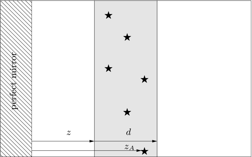
Figure 1: Amplifying slab consisting of a gas of excited atoms in front of perfect mirror.

The associated Green tensor reads Sambale et al. (2008a)

$$G_{xx}^{(1)}(z_{A},z_{A},\omega_{10}) =G_{yy}^{(1)}(z_{A},z_{A},\omega_{10})$$

$$=\frac{\omega_{10}e^{i\tilde{z}}}{4\pi c\tilde{z}^{3}}\left(1-i\tilde{z}-\tilde{z}^{2}\right),$$ (54)

$$G_{zz}^{(1)}(z_{A},z_{A},\omega_{10})=\frac{\omega_{10}e^{i\tilde{z}}}{2\pi c\tilde{z}^{3}}\left(1-i\tilde{z}\right)$$ (55)

[$\tilde{z}=2\omega_{10}z_{A}/c$] were $z_{A}$ denotes the atom–mirror distance. We will only consider the dominant resonant component of the Casimir force, $\mathbf{F}\approx\mathbf{F}_{r}$. According to Eq. (47) together with (IV) the Casimir force per unit area on the weakly polarisable plate is given by

$$\mathbf{F}(z)= \frac{\mu_{0}}{3}\eta\omega_{10}^{2}|\mathbf{d}_{10}|^{2}\int_{z}^{z+d}\mathrm{d}z_{A}\frac{\partial}{\partial{z_{A}}}{\rm Re}\,G_{ii}^{(1)}(\mathbf{r}_{A},\mathbf{r}_{A},\omega)\mathbf{e}_{z}$$ (56)

$$\equiv \frac{\mu_{0}}{3}\eta\omega_{10}^{2}|\mathbf{d}_{10}|^{2}H(\mathbf{z})\mathbf{e}_{z}$$ (57)

[$z$: plate–mirror distance, $\eta$: density of atoms in the plate] where

$$H(z)=\frac{\omega_{10}}{4\pi c\tilde{z}^{3}}\left[(2-\tilde{z}^{2})\cos(\tilde{z})+2\tilde{z}\sin(\tilde{z})\right]_{z_{A}=z}^{z_{A}=z+d}.$$ (58)

Fig. (2) shows the (dimensionless) Casimir force per thickness $d$ of the plate as a function of the atom–plate separation. For reference, we have also displayed the resonant part of the CP force on the individual atoms contained in the plate. It is seen that the Casimir force on the amplifying plate shows an attractive behaviour in the short-distance regime while for big plate–mirror separations an oscillating behavior can be found. This is a direct consequence of the respective behaviour of the CP forces on the atoms contained in the plate. The amplitude of the oscillations decreases with increasing thickness of the plate, since the integrated Casimir force per plate thickness is a spatial average of the oscillating CP forces over the plate thickness. The occurrence of oscillations can be regarded as the typical impact of amplification on the Casimir force.

Figure 2: Resonant Casimir force (per thickness $d$) between a planar sample of excited gas atoms and a perfect mirror plotted vs. the plate–mirror distance. The atomic dipole moments are oriented parallel to the surface. The solid line shows the resonant CP force on each excited atom.

VI Summary

Starting from the quantisation of the electromagnetic field in the presence of arbitrary linearly and locally responding media we have derived formulas for Casimir forces in a partially amplifying arrangement of (isotropic) magnetoelectric bodies of arbitrary shapes. Treating the Casimir force in the Lorentz force approach we have found that it can be decomposed into two parts; one that looks formally the same as in the case of purely absorbing body and can be regarded as an off-resonant force component due to the integration over the full frequency range and, a second, resonant part of the Casimir force that is a direct consequence of the amplification in the system and contains an integration over the frequencies where the imaginary part of the electric permittivity and/or (para)magnetic permeability is negative. These off-resonant and resonant parts of the Casimir force have a simple physical interpretation in the case of a partially amplifying object consisting of weak polarisable/magnetisable material in a purely absorbing environment. We have demonstrated that in this approximation the Casimir force can be written as a summation of pairwise CP forces on the excited atoms the body consists of; where the off-resonant/resonant contribution to the Casimir force could be related to the off-resonant/resonant CP force. These in turn are associated with virtual and real transitions of the excited atoms. As an example, we have studied the Casimir force between a weakly polarisable plate of excited gas atoms and a perfectly reflecting mirror. We have found attraction to the surface for small mirror–plate separation while the retarded regime is dominated by an oscillating behaviour as a consequence of the spatial average of the respective CP forces of the excited gas atoms.

The theory can be expanded to allow for linearly but non-locally responding anisotropic media. It can be used to evaluate the Casimir force beyond linear order in the susceptibilities.

References

• Lamoreaux (2005) S. K. Lamoreaux, Rep. Prog. Phys. 68, 201 (2005).
• Rockstuhl et al. (2007) C. Rockstuhl, F. Lederer, C. Etrich, T. Pertsch, and T. Scharf, Phys. Rev. Lett. 99, 017401 (2007).
• Liu et al. (2008) N. Liu, H. Guo, L. Fu, S. Kaiser, H. Schweizer, and H. Giessen, Nature Mat. 7, 31 (2008).
• Yang and Li (2008) Y. Yang and G. Li, Q. Wang (2008).
• Smith et al. (2000) D. R. Smith, W. J. Padilla, D. C. Vier, S. C. Nemat-Nasser, and S. Schultz, Phys. Rev. Lett. 84, 4184 (2000).
• Shelby et al. (2001) R. A. Shelby, D. R. Smith, S. C. Nemat-Nasser, and S. Schultz, App. Phys. Lett. 78, 489 (2001).
• Lezec et al. (2007) H. J. Lezec, J. A. Dionne, and H. A. Atwater, Sci. 316, 430 (2007).
• Paul et al. (2008) O. Paul, C. Imhof, B. Reinhard, R. Zengerle, and R. Beigang, Opt. Expr. 16, 6736 (2008).
• Buhmann et al. (2005) S. Y. Buhmann, D.-G. Welsch, and T. Kampf, Phys. Rev. A 72, 032112 (2005).
• Spagnolo et al. (2007) S. Spagnolo, D. A. R. Dalvit, and P. W. Milonni, Phys. Rev. A 75, 052117 (2007).
• Rosa et al. (2008) F. S. S. Rosa, D. A. R. Dalvit, and P. W. Milonni, Phys. Rev. Lett. 100, 183602 (2008).
• Yang et al. (2008) Y. Yang, R. Zeng, J. Xu, and S. Liu, Phys. Rev. A 77, 015803 (2008).
• Henkel and Joulain (2005) C. Henkel and K. Joulain, Europhys. Lett. 72, 929 (2005).
• Tomaš (2005a) M. S. Tomaš, Phys. Lett. A 342, 381 (2005a).
• Power and Thirunamachandran (1995a) E. A. Power and T. Thirunamachandran, Phys. Rev. A 51, 3660 (1995a).
• Rizzuto et al. (2004) L. Rizzuto, R. Passant, and F. Persico, Phys. Rev. A 70, 012107 (2004).
• Sherkunov (2005) Y. Sherkunov, Phys. Rev. A 72, 052703 (2005).
• Power and Thirunamachandran (1995b) E. Power and T. Thirunamachandran, Chem. Phys. 198, 5 (1995b).
• Passante et al. (2005) R. Passante, F. Persico, and L. Rizzuto, J. of Mod. Opt. 52, 1957 (2005).
• Sherkunov (2007a) Y. Sherkunov, J. of Phys. D: App. Phys. 40, 86 (2007a).
• Wylie and Sipe (1984) J. M. Wylie and J. E. Sipe, Phys. Rev. A 30, 185 (1984).
• Buhmann et al. (2004a) S. Y. Buhmann, L. Knöll, D.-G. Welsch, and Ho Trung Dung, Phys. Rev. A 70, 052117 (2004a).
• Sherkunov (2007b) Y. Sherkunov, Phy. Rev. A 75, 012705 (2007b).
• Sambale et al. (2008a) A. Sambale, D.-G. Welsch, Ho Trung Dung, and S. Y. Buhmann, arxiv 0711.3369, submitted to Phys. Rev. A (2008a).
• Sambale et al. (2008b) A. Sambale, S. Y. Buhmann, Ho Trung Dung, and D.-G. Welsch, arXiv 0809.3086, to be published in Phys. Scripta (2008b).
• Sandoghdar et al. (1992) V. Sandoghdar, C. I. Sukenik, E. A. Hinds, and S. Haroche, Phys. Rev. Lett. 68, 3432 (1992).
• Chevrollier et al. (2001) M. Chevrollier, M. Oria, J. G. de Souza, D. Bloch, M. Fichet, and M. Ducloy, Phys. Rev. E 63, 046610 (2001).
• Failache et al. (2003) H. Failache, S. Altiel, M. Fichet, D. Bloch, and M. Ducloy, Eur. Phys. J. D 23, 237 (2003).
• Ninham and Daicic (1998) B. Ninham and J. Daicic, Phys. Rev. A 57, 1870 (1998).
• Mostepanenko et al. (2006) V. M. Mostepanenko, V. B. Bezerra, R. S. Decca, B. Geyer, E. Fischbach, G. L. Klimchitskaya, D. E. Krause, and D. Lòpez, J. of Phys. A: Mathematical and General 39, 6589 (2006).
• Decca et al. (2005) R. S. Decca, D. López, E. Fischbach, G. L. Klimchitskaya, D. E. Krause, and V. Mostepanenko, Ann. Phys. NY 318, 37 (2005).
• Klimchitskaya et al. (2005) G. L. Klimchitskaya, R. S. Decca, E. Fischbach, D. E. Krause, D. López, and V. Mostepanenko, Int. J. Mod. Phys. A 20, 2205 (2005).
• McLachlan (1963) A. McLachlan, Proc. R. Soc. Lond. Ser. A 274 (1963).
• Henkel et al. (2002) C. Henkel, K. Joulain, J.-P. Mulet, and J.-J. Greffet, J. Opt. A: Pure Appl. Opt. 4, S109 (2002).
• Gorza and Ducloy (2006) M.-P. Gorza and M. Ducloy, Eur. Phys. J. D 40, 343 (2006).
• Antezza et al. (2005) M. Antezza, L. P. Pitaevskii, and S. Stringari, Phys. Rev. Lett. 95, 113202 (2005).
• Harber et al. (2005) D. M. Harber, J. M. Obrecht, J. M. McGuirk, and E. A. Cornell, Phys. Rev. A 72, 033610 (2005).
• Obrecht et al. (2007) J. M. Obrecht, R. J. Wild, M. Antezza, L. P. Pitaevskii, S. Stringari, and E. A. Cornell, Phys. Rev. Lett. 98, 063201 (2007).
• Buhmann and Scheel (2008a) S. Y. Buhmann and S. Scheel, arxiv: 0803.0738 (2008a).
• Sherkunov (2008) Y. Sherkunov, arxiv: 0608.2620 (2008).
• Scully and Zubairy (1997) M. Scully and M. S. Zubairy, Quantum optics (Cambr. Univ. Press, 1997).
• Popov and Shalaev (2006) A. K. Popov and V. M. Shalaev, Opt. Lett. 31, 2169 (2006).
• Stockmann (2007) M. Stockmann, Phys. Rev. Lett. 98, 177404 (2007).
• Leonhardt and Philbin (2007) U. Leonhardt and T. G. Philbin, N. J. of Phys. 9, 254 (2007).
• Zhao (2003) Y. P. Zhao, Acta Mechanica Sinica 19, 1 (2003).
• Raabe and Welsch (2008) C. Raabe and D.-G. Welsch, The Eur. Phys. J. - Special Topics 160, 371 (2008).
• Jeffers et al. (1996) J. Jeffers, S. M. Barnett, R. Loudon, R. Matloob, and M. Artoni, Opt. Commun. 131, 66 (1996).
• Matloob et al. (1997) R. Matloob, R. Loudon, M. Artoni, S. M. Barnett, and J. Jeffers, Phys. Rev. A 55, 1623 (1997).
• Kubo et al. (1998) R. Kubo, M. Toda, and N. Hashitsume, Statistical Physics II: Nonequilibrium Statistical Mechanics (Springer Verlag Berlin, 1998).
• Melrose and McPhedran (2003) D. B. Melrose and R. C. McPhedran, Electromagnetic processes in dispersive media : A treatment based on the dielectric tensor (Cambridge Univ. Press,, 2003).
• Scheel et al. (1998) S. Scheel, L. Knöll, and D.-G. Welsch, Phys. Rev. A 58, 700 (1998).
• Raabe and Welsch (2006) C. Raabe and D.-G. Welsch, Phys. Rev. A 73, 063822 (2006), note erratum Phys. Rev. A 74 (1) (2006) 019901(E) .
• Buhmann et al. (2004b) S. Y. Buhmann, Ho Trung Dung, and D.-G. Welsch, J. Opt. B: Quantum and Semiclassical Optics 6, 127 (2004b).
• Buhmann and Scheel (2008b) S. Y. Buhmann and S. Scheel, arxiv 0806.2211 (2008b).
• Tomaš (2005b) M. Tomaš, Phys. Rev. A 71, 060101(R) (2005b).
• Buhmann et al. (2006) S. Y. Buhmann, H. Safari, D.-G. Welsch, and Ho Trung Dung, Open Sys. & Information Dyn. 13, 427 (2006).
• Buhmann and Welsch (2006) S. Y. Buhmann and D.-G. Welsch, Appl. Phys. B 82, 189 (2006).
• Tomaš (1995) M. S. Tomaš, Phys. Rev. A 51, 2545 (1995).