Higher-order effects and ultra-short solitons in left-handed metamaterials

Abstract

Starting from Maxwell’s equations, we use the reductive perturbation method to derive a second-order and a third-order nonlinear Schrödinger equation, describing ultra-short solitons in nonlinear left-handed metamaterials. We find necessary conditions and derive exact bright and dark soliton solutions of these equations for the electric and magnetic field envelopes.

Electromagnetic (EM) properties of metamaterials with simultaneously negative permittivity $\epsilon$ and permeability $\mu$ have recently become a subject of intense research activity. Such metamaterials were experimentally realized recently in the microwave regime, by means of periodic arrays of small metallic wires and split-ring resonators (SRRs) exp . Many aspects of this class and other related types of metamaterials have been investigated, and various potential applications have been proposed reviews . So far, metamaterials have been mainly studied in the linear regime, where $\epsilon$ and $\mu$ do not depend on the EM field intensities. Nevertheless, nonlinear metamaterials, which may be created by embedding an array of wires and SRRs into a nonlinear dielectric zharov ; agranovich ; shadrivov , may prove useful in various applications. These include “switching” the material properties from left- to right-handed and back, tunable structures with intensity-controlled transmission, negative refraction photonic crystals, and so on.

EM wave propagation in nonlinear metamaterials can be described by two coupled nonlinear Schrödinger (NLS) equations for the EM field envelopes lazarides-tsironis . Thus, bright-bright and dark-dark vector solitons of the Manakov type manakov are supported in the right-handed (RH) and left-handed (LH) regimes, respectively lazarides-tsironis . These findings paved the way for relevant studies, e.g., modulational instability kourakis , and bright-dark vector solitons shukla in negative-index media. Additionally, a scalar higher-order NLS (HNLS) equation was derived in scalora (assuming nonlinear response only in the electric properties of the metamaterial), and was subsequently studied wen-pre ; shukla2 . Coupled HNLS equations were also derived wen-pra , where higher-order dispersion and nonlinear effects were included. However, the relative importance of these effects was not studied in Ref. wen-pra , although such an investigation should provide the necessary conditions for the formation of few-cycle pulses in nonlinear metamaterials.

In this work, we present a systematic derivation of NLS and HNLS equations for the EM field envelopes, as well as ultra-short solitons for left-handed (LH) metamaterials. In particular, we use the reductive perturbation method rpm to derive from Faraday’s and Ampére’s Laws a hierarchy of equations. Using such an approach, i.e., directly analyzing Maxwell’s equations, we show that the electric field envelope is proportional to the magnetic field one (their ratio being the linear wave-impedance). Thus, for each of the EM wave components we derive a single NLS (for moderate pulse widths) or a single HNLS equation (for ultra-short pulse widths), rather than a system of coupled NLS equations (as in Refs. lazarides-tsironis ; kourakis ; shukla ; wen-pra ). The HNLS equation, which incorporates higher-order dispersive and nonlinear terms, generalizes the one describing short pulse propagation in nonlinear optical fibers potasek ; kodhas ; potasek2 ; hasbook . Analyzing the NLS and HNLS equations, we find necessary conditions for the formation of bright or dark solitons in the LH regime, and derive analytically approximate ultra-short solitons in nonlinear metamaterials.

We consider lossless nonlinear metamaterials, characterized by the effective permittivity and permeability zharov ,

$$\epsilon(\omega) = \epsilon_{0}\bigg{(}\epsilon_{D}(|\mathbf{E}|^{2})-\frac{\omega_{p}^{2}}{\omega^{2}}\bigg{)},\quad\quad$$ (1)

$$\mu(\omega) = \mu_{0}\bigg{(}1-\frac{F\omega^{2}}{\omega^{2}-\omega_{0NL}^{2}(|\mathbf{H}|^{2})}\bigg{)},\qquad$$ (2)

where $\omega_{p}$ is the plasma frequency, F is the filling factor, $\omega_{0NL}$ is the nonlinear resonant SRR frequency zharov , while $\mathbf{E}$ and $\mathbf{H}$ are the electric and magnetic field intensities, respectively. In the linear limit, $\epsilon_{D}\rightarrow 1$ and $\omega_{0NL}\rightarrow\omega_{\rm res}$ (where $\omega_{\rm res}$ is the linear resonant SRR frequency), and LH behavior occurs in the frequency band $\omega_{\rm res}<\omega<{\rm min}\{\omega_{p},\omega_{M}\}$, with $\omega_{M}=\omega_{\rm res}/\sqrt{1-F}$, provided that $\omega_{p}>\omega_{\rm res}$. On the other hand, a weakly nonlinear behavior of the metamaterial can be approximated by the decompositions lazarides-tsironis ; kourakis ; scalora ; yskss :

$$\epsilon(\omega) = \epsilon_{L}(\omega)+\epsilon_{NL}(\omega;|\mathbf{E}|^{2}),$$ (3)

$$\mu(\omega) = \mu_{L}(\omega)+\mu_{NL}(\omega;|\mathbf{H}|^{2}),$$ (4)

where $\epsilon_{L}=\epsilon_{0}(1-\omega_{p}^{2}/\omega^{2})$, $\mu_{L}=\mu_{0}[1-F\omega^{2}/(\omega^{2}-\omega_{\rm res}^{2})]$, while the nonlinear parts of the permittivity and permeability are given by lazarides-tsironis ; kourakis ; scalora ; yskss : $\epsilon_{NL}(|\mathbf{E}|^{2})=\epsilon_{0}\alpha|\mathbf{E}|^{2}$, and $\mu_{NL}(|\mathbf{H}|^{2})=\mu_{0}\beta|\mathbf{H}|^{2}$; here, $\alpha=\pm E_{c}^{-2}$ and $\beta$ are the Kerr coefficients for the electric and magnetic fields, respectively, $E_{c}$ being a characteristic electric field value. The approximations (3)-(4) are physically justified considering that the slits of the SRRs are filled with a nonlinear dielectric zharov ; shadrivov . Generally, both cases of focusing and defocusing dielectrics (corresponding, respectively, to $\alpha>0$ and $\alpha<0$) are possible. The magnetic Kerr coefficient $\beta$ can be found via the dependence of $\mu$ on the magnetic field intensity zharov ; shadrivov . Here, fixing $F=0.4$ and $\omega_{p}=2\pi\times 10$ GHz, we will perform our analysis in the frequency band from $2\pi\times 1.45$ GHz to $2\pi\times 1.87$ GHz, considered also in Ref. lazarides-tsironis . In this band, SRRs are LH media (with $\epsilon_{L}<0$ and $\mu_{L}<0$ – see Fig. 1), $\alpha$ may be either positive or negative, while $\beta$ is positive lazarides-tsironis . Notice that, in principle, $\epsilon_{NL}$ and $\mu_{NL}$ may depend on both intensities $|\mathbf{E}|^{2}$ and $|\mathbf{H}|^{2}$; such a case can also be studied via the analytical approach we use below.

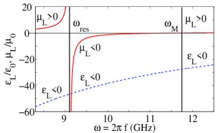
Figure 1: (Color online) The linear parts of the relative magnetic permeability, $\mu_{L}/\mu_{0}$ [solid (red) line], and the electric permittivity, $\epsilon_{L}/\epsilon_{0}$ [dashed (blue) line] as functions of frequency, for $F=0.4$ and $\omega_{p}=2\pi\times 10$ GHz.

We consider the propagation along the $+\hat{\mathbf{z}}$ direction of a $x$- ($y$-) polarized electric (magnetic) field, namely, $\mathbf{E}(z,t)=\hat{\mathbf{x}}E(z,t)$ and $\mathbf{H}(z,t)=\hat{\mathbf{y}}H(z,t)$. Then, using the constitutive relations (in frequency domain) $\mathbf{D}$=$\epsilon\mathbf{E}$ and $\mathbf{B}$=$\mu\mathbf{H}$ ($\mathbf{D}$ and $\mathbf{B}$ are the electric flux density and the magnetic induction), Faraday’s and Ampére’s Laws respectively read (in the time domain):

$$\partial_{z}E=-\partial_{t}(\mu\ast H),\,\,\,\,\,\partial_{z}H=-\partial_{t}(\epsilon\ast E),$$ (5)

where $\ast$ denotes the convolution integral, i.e., $f(t)\ast g(t)=\int_{-\infty}^{+\infty}f(\tau)g(t-\tau)d\tau$. Note that Eqs. (5) may be used in either the RH or the LH regime: once the dispersion relation $k_{0}=k_{0}(\omega_{0})$ (for the wavenumber $k_{0}$ and frequency $\omega_{0}$) and the evolution equations for the fields $E$ and $H$ are found, then $k_{0}>0$ ($k_{0}<0$) corresponds to the RH (LH) regime. Alternatively, for fixed $k_{0}>0$, one should shift the fields as $[E,H]^{T}\rightarrow[\pm E,\mp H]^{T}$, thus inverting the orientation of the magnetic field and associated Poynting vector. Here, we will assume that the wavenumber $k_{0}$ [see Eq. (22) below] will be $k_{0}<0$ for the LH regime.

Now, we consider that the fields are expressed as $[E(z,t),H(z,t)]^{T}=[q(z,t),p(z,t)]^{T}\exp[i(k_{0}z-\omega_{0}t)]$, where $q$ and $p$ are unknown field envelopes. Nonlinear evolution equations for the latter can be found by the reductive perturbation method rpm as follows. First, we assume that the temporal spectral width of the nonlinear term with respect to that of the quasi-plane-wave dispersion relation is characterized by the small parameter $\varepsilon$ potasek ; kodhas ; potasek2 ; hasbook . Then, we introduce the slow variables:

$$Z=\varepsilon^{2}z,\quad\quad T=\varepsilon(t-k_{0}^{\prime}z),$$ (6)

where $k_{0}^{\prime}\equiv v_{g}^{-1}$ is the inverse of the group velocity (hereafter, primes will denote derivatives with respect to $\omega_{0}$). Additionallly, we express $q$ and $p$ as asymptotic expansions in terms of the parameter $\varepsilon$,

$$q(Z,T)= q_{0}(Z,T)+\varepsilon q_{1}(Z,T)+\varepsilon^{2}q_{2}(Z,T)+\cdots,$$ (7)

$$p(Z,T)= p_{0}(Z,T)+\varepsilon p_{1}(Z,T)+\varepsilon^{2}p_{2}(Z,T)+\cdots,$$ (8)

and assume that the Kerr coefficients $\alpha$ and $\beta$ are of order $\mathcal{O}(\varepsilon^{2})$ (see, e.g., lazarides-tsironis ; potasek ; kodhas ). Substituting Eqs. (7)-(8) into Eqs. (5), using Eqs. (3), (4), and (6), and Taylor expanding the functions $\epsilon_{L}$, and $\mu_{L}$, we arrive at the following equations at various orders of $\varepsilon$:

$$\mathcal{O}(\varepsilon^{0}):\,\,\mathbf{W}\mathbf{x}_{0} = \mathbf{0},$$ (9)

$$\mathcal{O}(\varepsilon^{1}):\,\,\mathbf{W}\mathbf{x}_{1} = -i\mathbf{W}^{\prime}\partial_{T}\mathbf{x}_{0},$$ (10)

$$\mathcal{O}(\varepsilon^{2}):\,\,\mathbf{W}\mathbf{x}_{2} = -i\mathbf{W}^{\prime}\partial_{T}\mathbf{x}_{1}+\frac{1}{2}\mathbf{W}^{\prime\prime}\partial^{2}_{T}\mathbf{x}_{0}$$

$$+ \frac{1}{2}k_{0}^{\prime\prime}\partial^{2}_{T}\mathbf{x}_{0}-i\partial_{Z}\mathbf{x}_{0}-\mathbf{A}\mathbf{x}_{0},$$ (11)

$$\mathcal{O}(\varepsilon^{3}):\,\,\mathbf{W}\mathbf{x}_{3} = -i\mathbf{W}^{\prime}\partial_{T}\mathbf{x}_{2}+\frac{1}{2}\mathbf{W}^{\prime\prime}\partial^{2}_{T}\mathbf{x}_{1}+\frac{i}{6}\mathbf{W}^{\prime\prime\prime}\partial^{3}_{T}\mathbf{x}_{0}$$ (12)

$$+ \frac{i}{6}k_{0}^{\prime\prime\prime}\partial^{3}_{T}\mathbf{x}_{0}+\frac{1}{2}k_{0}^{\prime\prime}\partial^{2}_{T}\mathbf{x}_{1}-i\partial_{Z}\mathbf{x}_{1}$$

$$- \mathbf{A}\mathbf{x}_{1}+i\mathbf{B}\mathbf{x}_{0},$$

with $\mathbf{x}_{i}=\left[q_{i},p_{i}\right]^{\mathrm{T}}$ ($i=0,1,2,3$) unknown vectors, and

$$\mathbf{W}= \left[\begin{array}[]{cc}-k_{0}&\omega_{0}\mu_{L}\\ \omega_{0}\epsilon_{L}&-k_{0}\\ \end{array}\right],\,\,\,\,\,\,\mathbf{A}\mathbf{x}_{i}=\omega_{0}\left[\begin{array}[]{c}\beta|p_{0}|^{2}p_{i}\\ \alpha|q_{0}|^{2}q_{i}\\ \end{array}\right],$$ (17)

$$\mathbf{B}\mathbf{x}_{0}= \left[\begin{array}[]{c}-\beta\partial_{T}(|p_{0}|^{2}p_{0})+i\omega_{0}\beta(p_{0}p_{1}^{\star}+p_{0}^{\star}p_{1})p_{0}\\ -\alpha\partial_{T}(|q_{0}|^{2}q_{0})+i\omega_{0}\alpha(q_{0}q_{1}^{\star}+q_{0}^{\star}q_{1})q_{0}\\ \end{array}\right],$$ (20)

with $\star$ denoting complex conjugate. To proceed further, we note that the compatibility conditions required for Eqs. (9)-(12) to be solvable, known also as Fredholm alternatives rpm ; kodhas , are $\mathbf{L}\mathbf{W}\mathbf{x}_{i}=0$, where $\mathbf{L}=[1,Z_{L}]$ is a left eigenvector of of $\mathbf{W}$, such that $\mathbf{L}\mathbf{W}=\mathbf{0}$, with $Z_{L}=\sqrt{\mu_{L}/\epsilon_{L}}$ being the linear wave-impedance.

The leading-order Eq. (9) provides the following results. First, the solution $\mathbf{x}_{0}$ of Eq. (9) has the form:

$$\mathbf{x}_{0}=\mathbf{R}\phi(Z,T),$$ (21)

where $\phi(Z,T)$ is an unknown scalar field and $\mathbf{R}=[1,Z_{L}^{-1}]^{\rm T}$ is a right eigenvector of $\mathbf{W}$, such that $\mathbf{W}\mathbf{R}=\mathbf{0}$. Second, by using the compatibility condition $\mathbf{L}\mathbf{W}\mathbf{x}_{0}=0$ and Eq. (21), we obtain the equation $\mathbf{L}\mathbf{W}\mathbf{R}=0$, which is actually the linear dispersion relation,

$$k_{0}^{2}=\omega_{0}^{2}\epsilon_{L}\mu_{L},$$ (22)

($\epsilon_{L}$ and $\mu_{L}$ are evaluated at $\omega_{0}$). Note that Eq. (22) is also obtained by imposing the nontrivial solution condition ${\rm det}\mathbf{W}=0$. Third, the EM field envelopes are proportional to each other, i.e., $q_{0}=p_{0}Z_{L}$.

At $\mathcal{O}(\varepsilon^{1})$, the compatibility condition for Eq. (10) results in $\mathbf{L}\mathbf{W}^{\prime}\mathbf{R}=0$, written equivalently as:

$$2k_{0}k_{0}^{\prime}=\omega_{0}^{2}(\epsilon_{L}\mu^{\prime}_{L}+\epsilon^{\prime}_{L}\mu_{L})+2\omega_{0}\epsilon_{L}\mu_{L}.$$ (23)

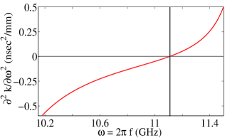
Figure 2: (Color online) The GVD coefficient $k^{\prime\prime}\equiv\partial^{2}k/\partial\omega^{2}$ as a function of frequency in the left-handed regime.

This is actually the definition of the group velocity $v_{g}=1/k_{0}^{\prime}$, as can also be found by differentiating Eq. (22) with respect to $\omega$. Furthermore, using Eq. (21), Eq. (10) suggests that the unknown vector $\mathbf{x}_{1}$ has the form,

$$\mathbf{x}_{1}=i\mathbf{R}^{\prime}\partial_{T}\phi(Z,T)+\mathbf{R}\psi(Z,T),$$ (24)

where $\psi(Z,T)$ is an unknown scalar field.

Next, at order $\mathcal{O}(\varepsilon^{2})$, the compatibility condition for Eq. (11), combined with Eqs. (21) and (24), yields the following NLS equation,

$$i\partial_{Z}\phi-\frac{1}{2}k_{0}^{\prime\prime}\partial_{T}^{2}\phi+\gamma|\phi|^{2}\phi=0,$$ (25)

where $k_{0}^{\prime\prime}$ is the group-velocity dispersion (GVD) coefficient, as can be evaluated by differentiating $k_{0}^{\prime}$ in Eq. (23), and $\gamma=(\omega_{0}^{2}/2k_{0})(\epsilon_{0}\alpha\mu_{L}+\mu_{0}\beta\epsilon_{L}Z_{L}^{-2})$. Note that once $\phi$ is obtained from the NLS Eq. (25), the EM field envelopes are determined as $q_{0}=\phi$ and $p_{0}=Z_{L}^{-1}\phi$ [see Eq. (21)], similarly to the case of a linear medium.

Finally, to order $\mathcal{O}(\varepsilon^{3})$, we use the compatibility condition for Eq. (12), as well as Eqs. (11), (21) and (24), and obtain a NLS equation, incorporating higher-order dispersive and nonlinear terms. This equation describes the evolution of $\psi$, and yet contains $\phi$, which in turn obeys Eq. (25). Instead of considering this system of two equations, we follow potasek ; kodhas ; hasbook and introduce a new combined function $\Phi=\phi+\varepsilon\psi$. This way, combining the NLS equations obtained at orders $\mathcal{O}(\varepsilon^{2})$ and $\mathcal{O}(\varepsilon^{3})$, we find that $\Phi$ obeys the HNLS equation:

$$i\partial_{Z}\Phi -\frac{1}{2}k_{0}^{\prime\prime}\partial_{T}^{2}\Phi+\gamma|\Phi|^{2}\Phi$$

$$=i\varepsilon\left[\frac{1}{6}k_{0}^{\prime\prime\prime}\partial_{T}^{3}\Phi-\frac{\gamma}{\omega_{0}}\partial_{T}(|\Phi|^{2}\Phi)\right].$$ (26)

For $\varepsilon=0$, the HNLS Eq. (26) is reduced to the NLS Eq. (25), while for $\varepsilon\neq 0$ generalizes the higher-order NLS equation describing ultra-short pulse propagation in optical fibers potasek ; kodhas ; potasek2 ; hasbook (where dispersion and nonlinearity appear solely in the dielectric properties). As in the NLS Eq. (25), Eq. (26) provides the field $\Phi$ which, in turn, determines the EM fields at order $\mathcal{O}(\varepsilon^{3})$ as $q_{0}+\varepsilon q_{1}=\Phi$ and $p_{0}+\varepsilon p_{1}=Z_{L}^{-1}\Phi$ [see Eqs. (21), (24)]. Finally, we stress that the NLS Eq. (25), or the HNLS Eq. (26), can be used in the LH (RH) regime, taking $k_{0}$, $\epsilon_{L}$, and $\mu_{L}$ negative (positive) as per the discussion above.

Table 1: Conditions for the formation of bright or dark solitons (BS or DS) for the NLS Eq. (27).

		$s=+1$	$s=-1$
$\sigma=+1$	$\alpha>0$	DS	BS
$\sigma=-1$	$\alpha<0$,  $|\frac{\alpha}{\beta}|>\frac{Z_{0}^{2}}{Z_{L}^{4}}$	BS	DS
$\sigma=+1$	$\alpha<0$,  $|\frac{\alpha}{\beta}|<\frac{Z_{0}^{2}}{Z_{L}^{4}}$	DS	BS

Let us now analyze Eqs. (25) and (26) in more detail. First, measuring length, time, and the field intensity $|\phi|^{2}$ in units of the dispersion length $L_{D}=t_{0}^{2}/|k_{0}^{\prime\prime}|$, initial pulse width $t_{0}$, and $L_{D}/|\gamma|$, respectively, we reduce the NLS Eq. (25) to the following dimensionless form:

$$i\partial_{Z}\phi-\frac{s}{2}\partial_{T}^{2}\phi+\sigma|\phi|^{2}\phi=0,$$ (27)

where $s={\rm sign}(k_{0}^{\prime\prime})$ and $\sigma={\rm sign}(\gamma)$. The NLS Eq. (27) admits bright (dark) soliton solutions for $s\sigma=-1$ ($s\sigma=+1$). As is shown in Fig. 2, for our choice of parameters, $s=+1$ (i.e., $k_{0}^{\prime\prime}>0$) for $2\pi\times 1.76<\omega<2\pi\times 1.87$ GHz, while $s=-1$ (i.e., $k_{0}^{\prime\prime}<0$) for $2\pi\times 1.45<\omega<2\pi\times 1.76$ GHz in the LH regime. Moreover, since $\beta>0$, we have $\sigma=+1$ either for a focusing dielectric, $\alpha>0$, or for a defocusing dielectric, $\alpha<0$, with $|\alpha/\beta|<Z_{0}^{2}/Z_{L}^{4}$ ($Z_{0}=\sqrt{\mu_{0}/\epsilon_{0}}$ is the vacuum wave-impedance). Hence, for $\sigma=+1$, bright (dark) solitons occur in the anomalous (normal) dispersion regimes, i.e., for $k_{0}^{\prime\prime}<0$ ($k_{0}^{\prime\prime}>0$), respectively. On the other hand, $\sigma=-1$ for $\alpha<0$, with $|\alpha/\beta|>Z_{0}^{2}/Z_{L}^{4}$ and, bright (dark) solitons occur in the normal (anomalous) dispersion regimes. The above results are summarized in Table I. Note that the presence of dispersion and nonlinearity in the magnetic response of the metamaterial allows for bright (dark) solitons in the anomalous (normal) dispersion regimes for defocusing dielectrics (see third line of Table I).

Next, we consider the HNLS Eq. (26) which, by using the same dimensionless units as before, is expressed as,

$$i\partial_{Z}\Phi-\frac{s}{2}\partial_{T}^{2}\Phi+\sigma|\Phi|^{2}\Phi=i\delta_{1}\partial_{T}^{3}\Phi-i\sigma\delta_{2}\partial_{T}(|\Phi|^{2}\Phi),$$ (28)

where $\delta_{1}=\varepsilon k_{0}^{\prime\prime\prime}/(6t_{0}|k_{0}^{\prime\prime}|)$, and $\delta_{2}=\varepsilon/(\omega_{0}t_{0})$. Equation (28) can be used to predict ultra-short solitons in nonlinear LH metamaterials as follows. Following Ref. hizfrapol , we seek travelling-wave solutions of Eq. (28) of the form,

$$\Phi(Z,T)=U(\eta)\exp[i(KZ-\Omega T)],$$ (29)

where $U(\eta)$ is the unknown envelope function (assumed to be real), $\eta=T-\Lambda Z$, and the real parameters $\Lambda$, $K$ and $\Omega$ denote, respectively, the inverse velocity, wavenumber and frequency of the travelling wave. Substituting Eq. (29) into Eq. (28), the real and imaginary parts of the resulting equation respectively read:

$$\ddot{U}+\frac{K-\frac{s}{2}\Omega^{2}-\delta_{1}\Omega^{3}}{\frac{s}{2}+3\delta_{1}\Omega}U-\frac{\sigma(1+\delta_{2}\Omega)}{{\frac{s}{2}+3\delta_{1}\Omega}}U^{3}=0,$$ (30)

$$\delta_{1}\dddot{U}+(\Lambda-s\Omega-3\delta_{1}\Omega^{2})\dot{U}-3\sigma\delta_{2}U^{2}\dot{U}=0,$$ (31)

where overdots denote differentiations with respect to $\eta$. Notice that in the case of $\delta_{1}=\delta_{2}=0$, Eq. (31) is automatically satisfied if $\Lambda=s\Omega$ and the profile of “long” soliton pulses [governed by Eq. (27)] is determined by Eq. (30). On the other hand, for ultra-short solitons (corresponding to $\delta_{1}\neq 0$, $\delta_{2}\neq 0$), the system of Eqs. (30) and (31) is consistent if the following conditions hold:

$$\frac{K-\frac{s}{2}\Omega^{2}-\delta_{1}\Omega^{3}}{\frac{s}{2}+3\delta_{1}\Omega}=\frac{\Lambda-s\Omega-3\delta_{1}\Omega^{2}}{\delta_{1}}\equiv\kappa,$$ (32)

$$-\frac{\sigma\delta_{2}}{\delta_{1}}=-\frac{\sigma(1+\delta_{2}\Omega)}{\frac{s}{2}+3\delta_{1}\Omega}\equiv\nu,$$ (33)

where $\kappa$ and $\nu$ are nonzero constants. In such a case, Eqs. (30) and (31) are equivalent to the following equation of motion of the unforced and undamped Duffing oscillator,

$$\ddot{U}+\kappa U+\nu U^{3}=0.$$ (34)

For $\kappa\nu<0$, Eq. (34) possesses two exponentially localized solutions (as special cases of its general elliptic function solutions), corresponding to the separatrices in the $(U,\dot{U})$ phase-plane. These solutions have the form of a hyperbolic secant (tangent) for $\kappa<0$ and $\nu>0$ ($\kappa>0$ and $\nu<0$), thus corresponding to the bright, $U_{\rm BS}$ (dark, $U_{\rm DS}$) solitons of Eq. (28):

$$U_{\rm BS}(\eta) = \left(2|\kappa|/\nu\right)^{1/2}\mathrm{sech}(\sqrt{|\kappa|}\eta),\,\qquad$$ (35)

$$U_{\rm DS}(\eta) = \left(2\kappa/|\nu|\right)^{1/2}\mathrm{tanh}(\sqrt{\kappa/2}\eta).$$ (36)

These are ultra-short solitons of the HNLS Eq. (28), valid even for $\varepsilon=\mathcal{O}(1)$: since both coefficients $\delta_{1}$, $\delta_{2}$ of Eq. (28) scale as $\varepsilon(\omega_{0}t_{0})^{-1}$, it is clear that for $\omega_{0}t_{0}=\mathcal{O}(1)$, or for soliton widths $t_{0}\sim\omega_{0}^{-1}$, the higher-order terms can safely be neglected and soliton propagation is governed by Eq. (27). On the other hand, if $\omega_{0}t_{0}=\mathcal{O}(\varepsilon)$, the higher-order terms become important and solitons governed by the HNLS Eq. (28) are ultra-short, of a width $t_{0}\sim\varepsilon\omega_{0}^{-1}$. We stress that these solitons are approximate solutions of Maxwell’s equations, satisfying Faraday’s and Ampére’s Laws in Eqs. (5) up to order $\mathcal{O}(\varepsilon^{3})$.

Finally, as concerns the condition for bright or dark soliton formation, namely $\kappa\nu<0$, we note that $\kappa$ depends on the free parameters $K$ and $\Omega$ (and, thus, can be tuned on demand), while the parameter $\nu$ has the opposite sign from $\sigma$ (since $\delta_{2}>0$, while ${\rm sign}(\delta_{1})={\rm sign}(k_{0}^{\prime\prime\prime})=+1$ – see Fig. 2). This means that bright solitons are formed for $\kappa<0$ and $\sigma=-1$ (i.e., $\alpha<0$ with $|\alpha/\beta|>Z_{0}^{2}/Z_{L}^{4}$), while dark ones are formed for $\kappa>0$ and $\sigma=+1$ (i.e., $\alpha>0$, or $\alpha<0$ with $|\alpha/\beta|<Z_{0}^{2}/Z_{L}^{4}$).

In conclusion, we used the reductive perturbation method to derive from Maxwell’s equations a HNLS equation describing pulse propagation in nonlinear metamaterials. We studied the pertinent dispersive and nonlinear effects, found necessary conditions for the formation of bright or dark ultra-short solitons, as well as approximate analytical expressions for these solutions. Future research may include a systematic study of the stability and dynamics of the ultra-short solitons, both in the framework of the HNLS equation and, perhaps more importantly, in the context of Maxwell’s equations.

References

(1) D. R. Smith et al.,
Phys. Rev. Lett. 84, 4184 (2000);
D. R. Smith and N. Kroll,
Phys. Rev. Lett. 85, 2933 (2000);
A. Shelby, D. R. Smith, and S. Schultz,
Science 292, 77 (2001).
(2) D. R. Smith, J. B. Pendry, M. C. K. Wiltshire,
Science 305, 788 (2004);
C. M. Soukoulis, M. Kafesaki, and E.N. Economou, Adv. Materials 18, 1941 (2006);
G. V. Eleftheriades and K. G. Balmain (eds.) Negative-Refraction Metamaterials. Fundamental Principles
and Applications (John Wiley, New Jersey, 2005).
(3) A. A. Zharov, I. V. Shadrivov, and Yu. S. Kivshar,
Phys. Rev. Lett. 91, 037401 (2003).
(4) V. M. Agranovich et al.,
Phys. Rev. B 69, 165112 (2004).
(5) I. V. Shadrivov et al.,
Radio Sci. 40, RS3S90 (2005).
(6) N. Lazarides, and G. P. Tsironis,
Phys. Rev. E 71, 036614 (2005).
(7) S. V. Manakov, Zh. Eksp. Teor. Fiz. 65, 505
(1973) [Sov. Phys. JETP 38, 248 (1974)].
(8) I. Kourakis, and P. K. Shukla, Phys. Rev. E 72, 016626 (2005).
(9) M. Marklund et al.,
Phys. Lett. A 341, 231 (2005).
(10) M. Scalora et al.,
Phys. Rev. Lett. 95, 013902 (2005).
(11) S. C. Wen et al.,
Phys. Rev. E 73, 036617 (2006).
(12) M. Marklund, P. K. Shukla, and L. Stenflo, Phys. Rev. E 73, 037601 (2006).
(13) S. C. Wen et al.,
Phys. Rev. A 75, 033815 (2007).
(14) T. Taniuti, Prog. Theor. Phys. Suppl. 55, 1 (1974);
H. Leblond, J. Phys. B
41, 043001 (2008).
(15) Y. Kodama, J. Stat. Phys. 39, 597 (1985).
(16) Y. Kodama and A. Hasegawa, IEEE J. Quantum Electron. 23, 510 (1987).
(17) M. J. Potasek, J. Appl. Phys. 65, 941 (1989).
(18) A. Hasegawa and Y. Kodama, Solitons in Optical Communications
(Clarendon Press, Oxford, 1995).
(19) I. V. Shadrivov and Y. S. Kivshar, J. Opt. A: Pure Appl. Opt. 7, S68 (2005).
(20) K. Hizanidis, D. J. Frantzeskakis, and C. Polymilis, J. Phys. A: Math. Gen. 29, 7687 (1996).