Ultimate “SIR” in Autonomous Linear Networks with Symmetric Weight Matrices, and Its Use to Stabilize the Network - A Hopfield-like network

Zekeriya Uykan Z. Uykan is with Doğuş University, Electronics and Communications Engineering, Acibadem, 34722 Kadiköy, Istanbul, Turkey. He was with the Helsinki University of Technology, Control Engineering Laboratory, FI-02015 HUT, Finland, and with Nokia Siemens Networks, Espoo, Finland. E-mail: zuykan@dogus.edu.tr. He was a visiting scientist at Harvard University Broadband Comm Lab., Cambridge, 02138, MA, from September 2008 to June 2009 and the first version of this work was performed during his stay at Harvard University.
Abstract

In this paper, we present and analyse two Hopfield-like nonlinear networks, in continuous-time and discrete-time respectively. The proposed network is based on an autonomous linear system with a symmetric weight matrix, which is designed to be unstable, and a nonlinear function stabilizing the whole network thanks to a manipulated state variable called“ultimate SIR”. This variable is observed to be equal to the traditional Signal-to-Interference Ratio (SIR) definition in telecommunications engineering.

The underlying linear system of the proposed continuous-time network is 𝐱˙=𝐁𝐱˙𝐱𝐁𝐱\dot{{\mathbf{x}}}={\mathbf{B}}{\mathbf{x}} where B is a real symmetric matrix whose diagonal elements are fixed to a constant. The nonlinear function, on the other hand, is based on the defined system variables called “SIR”s. We also show that the “SIR”s of all the states converge to a constant value, called “system-specific Ultimate SIR”; which is equal to rλmax𝑟subscript𝜆𝑚𝑎𝑥\frac{r}{\lambda_{max}} where r𝑟r is the diagonal element of matrix 𝐁𝐁{\bf B} and λmaxsubscript𝜆𝑚𝑎𝑥\lambda_{max} is the maximum (positive) eigenvalue of diagonally-zero matrix (𝐁r𝐈)𝐁𝑟𝐈({\bf B}-r{\bf I}), where 𝐈𝐈{\bf I} denotes the identity matrix. The same result is obtained in its discrete-time version as well.

Computer simulations for binary associative memory design problem show the effectiveness of the proposed network as compared to the traditional Hopfield Networks.

Index Terms:
Autonomous Continuos/Discrete-Time Linear Systems, Hopfield Networks, Signal to Interference Ratio (SIR).

I Introduction

Hopfield Neural Networks [1] has been an important focus of research area in not only neural networks field but also circit and system theory since early 1980s whose applications vary from combinatorial optimization (e.g. [2], [3] among many others) including travelling salesman problem (e.g. [4], [5] among others) to image restoration (e.g. [6]), from various control engineering optimization problems including robotics (e.g. [8] among others) to associative memory systems (e.g. [7], [11] among others), etc. For a tutorial and further references about Hopfield NN, see e.g. [10] and [9].

In this paper, we present and analyse two Hopfield-like nonlinear networks, called SALU-SIR and DSALU-SIR in continuous-time and discrete-time respectively.

The proposed networks consist of linear and nonlinear parts: An autonomous linear system with a symmetric weight matrix, which is designed to be unstable, and a nonlinear function stabilizing the whole network. The underlying linear system of the proposed continuous time-network is

𝐱˙=𝐁𝐱˙𝐱𝐁𝐱\dot{{\mathbf{x}}}={\mathbf{B}}{\mathbf{x}} (1)

where 𝐱˙˙𝐱\dot{{\mathbf{x}}} shows the derivative of 𝐱𝐱{\mathbf{x}} with respect to time, i.e., 𝐱˙=d𝐱dt˙𝐱𝑑𝐱𝑑𝑡\dot{{\mathbf{x}}}=\frac{d{\mathbf{x}}}{dt}, and 𝐁𝐁{\mathbf{B}} is called system matrix or weight matrix.

We define the following system variables denoted as θisubscript𝜃𝑖\theta_{i},

θi(t)=biixi(t)di+j=1,jiNbijxj(t),i=1,,Nformulae-sequencesubscript𝜃𝑖𝑡subscript𝑏𝑖𝑖subscript𝑥𝑖𝑡subscript𝑑𝑖superscriptsubscriptformulae-sequence𝑗1𝑗𝑖𝑁subscript𝑏𝑖𝑗subscript𝑥𝑗𝑡𝑖1𝑁{\theta_{i}}(t)=\frac{b_{ii}x_{i}(t)}{d_{i}+\sum_{j=1,j\neq i}^{N}b_{ij}x_{j}(t)},\quad i=1,\dots,N (2)

where xi(t)subscript𝑥𝑖𝑡x_{i}(t) represents the i𝑖i’th neuron and bijsubscript𝑏𝑖𝑗b_{ij} is the ij𝑖𝑗ij’th element of matrix 𝐁𝐁{\mathbf{B}}. In this paper, we assume di=0subscript𝑑𝑖0d_{i}=0 for the sake of brevity.

We observe that the manipulated state variable θi(t)subscript𝜃𝑖𝑡{\theta_{i}}(t) of eq.(2) resembles the well-known Signal-to-Interference-Ratio (SIR) definition in telecommunicaions engineering, which can be found in any related texbooks: Signal-to-Interference Ratio (SIR) is an important entity in commucations engineering which indicates the quality of a link between a transmitter and a receiver in a multi transmitter-receiver environment (see e.g. [13], [18]). For example, let N𝑁N represent the number of transmitters and receivers using the same channel. Then the received SIR is given by (e.g. [13])

γi(t)=giipi(t)νi+j=1,jiNgijpj(t),i=1,,Nformulae-sequencesubscript𝛾𝑖𝑡subscript𝑔𝑖𝑖subscript𝑝𝑖𝑡subscript𝜈𝑖superscriptsubscriptformulae-sequence𝑗1𝑗𝑖𝑁subscript𝑔𝑖𝑗subscript𝑝𝑗𝑡𝑖1𝑁\gamma_{i}(t)=\frac{g_{ii}p_{i}(t)}{\nu_{i}+\sum_{j=1,j\neq i}^{N}g_{ij}p_{j}(t)},\quad i=1,\dots,N (3)

where pisubscript𝑝𝑖p_{i} is the transmission power of transmitter i𝑖i, gijsubscript𝑔𝑖𝑗g_{ij} is the link gain from transmitter j𝑗j to receiver i𝑖i (e.g. in case of wireless communications, gijsubscript𝑔𝑖𝑗g_{ij} involves path loss, shadowing, etc) and νisubscript𝜈𝑖\nu_{i} is the receiver noise at receiver i𝑖i. Typically in communication systems like cellular radio systems, every transmitter tries to optimize its power pisubscript𝑝𝑖p_{i} such that the received SIR (i.e., γisubscript𝛾𝑖\gamma_{i}) in eq.(3) is kept at a target SIR value, γitgtsuperscriptsubscript𝛾𝑖𝑡𝑔𝑡\gamma_{i}^{tgt}.

It is well-known that the eigenvalues of the system matrix solely determine the stability of a linear dynamic networks. If any of the eigenvalues is positive, then the system is unstable. Designing the linear part of the network to have positive eigenvalue(s), we show, in this paper, that the defined “SIR” in eq.(2) for any state appraches asymptotically to a constant, called “ultimate SIR”, which is a function of the diagonal entry of the system matrix and its maximum eigenvalue. The nonlinear part of the network uses this result to stabilize the system. Finally, the proposed network is shown to exhibit features which are generally attributed to Hopfield Networks. Taking the sign of the converged states, the proposed network is applied to binary associative memory systems design.

The paper is organized as follows: The “ultimate SIR” is analysed for the underlying linear dynamic part of the network with a symmetric weight matrix in section II. Section III presents the stabilized network by the Ultimate ”SIR” to be used as a binary associative memory system. Simulation results are presented in section IV followed by the conclusions in Section V.

II Ultimate “SIR” Analysis

In this section, we analyse the underlying linear system of the proposed network in both continuous-time and discrete-time respectively.

II-A Continuous-time Analysis

In this paper, we examine the case where weight matrix 𝐁𝐁{\mathbf{B}} in eq.(1) is a real symmetric matrix whose diagonal elements are equal to a constant. So, the linear system in (1) can be written as follows

𝐱˙=(r𝐈+𝐖)𝐱˙𝐱𝑟𝐈𝐖𝐱\dot{{\mathbf{x}}}=\Big{(}-r{\bf I}+{\mathbf{W}}\Big{)}{\bf x} (4)

where

r𝐈=[r000r0000r],and𝑟𝐈delimited-[]𝑟000𝑟0missing-subexpression000𝑟and\displaystyle r{\bf I}=\left[\begin{array}[]{c c c c}r&0&\ldots&0\\ 0&r&\ldots&0\\ \vdots&&\ddots&0\\ 0&0&\ldots&r\end{array}\right],\quad\quad\textrm{and} (9)
𝐖=[0w12w1Nw210w2NwN1wN20]𝐖delimited-[]0subscript𝑤12subscript𝑤1𝑁subscript𝑤210subscript𝑤2𝑁missing-subexpressionsubscript𝑤𝑁1subscript𝑤𝑁20\displaystyle{\mathbf{W}}=\left[\begin{array}[]{c c c c}0&w_{12}&\ldots&w_{1N}\\ w_{21}&0&\ldots&w_{2N}\\ \vdots&&\ddots&\vdots\\ w_{N1}&w_{N2}&\ldots&0\end{array}\right] (14)

where wij=wji,i,j=1,2,,Nformulae-sequencesubscript𝑤𝑖𝑗subscript𝑤𝑗𝑖𝑖𝑗12𝑁w_{ij}=w_{ji},\quad i,j=1,2,\dots,N.

In eq.(14), the design parameter r𝑟r, which corresponds to biisubscript𝑏𝑖𝑖b_{ii} in the ”SIR” (θisubscript𝜃𝑖{\theta_{i}}) definition in eq.(2), is positive, r>0𝑟0r>0. For the sake of brevity, we assume that the bi=0,i=1,2,,Nformulae-sequencesubscript𝑏𝑖0𝑖12𝑁b_{i}=0,\quad i=1,2,\dots,N in the analysis.

It’s well known that desigining the weight matrix 𝐖𝐖{\mathbf{W}} as a symmetric one yields that all eigenvalues are real (see e.g. [16]), which we assume throughout the paper for the sake of brevity of its analysis.

Proposition 1:

Let’s assume that the linear dynamic network of eq.(4) with a real symmetric 𝐖𝐖{\bf W} in (14) has positive eigenvalue(s). If r>0𝑟0r>0 is chosen such that it’s smaller than the maximum (positive) eigenvalue of 𝐖𝐖{\bf W}, then

  1. 1.

    the defined ”SIR” (θisubscript𝜃𝑖{\theta_{i}}) in eq.(2) for any state i𝑖i asymptotically converges to the following constant as time evolves for any initial vector 𝐱(0)𝐱0{\bf x}(0) which is not completely perpendicular to the eigenvector corresponding to the largest eigenvalue of 𝐖𝐖{\bf W}. 111 It’s easy to check in advance if the initial vector 𝐱(0)𝐱0{\bf x}(0) is completely perpendicular to the eigenvector of the maximum (positive) eigenvalue of 𝐖𝐖{\bf W} or not. If this is the case, then this can easily be overcome by introducing a small random number to 𝐱(0)𝐱0{\bf x}(0) so that it’s not completely perpendicular to the mentioned eigenvector.

    θiult=θult=rλmax,i=1,2,,Nformulae-sequencesuperscriptsubscript𝜃𝑖𝑢𝑙𝑡superscript𝜃𝑢𝑙𝑡𝑟subscript𝜆𝑚𝑎𝑥𝑖12𝑁\theta_{i}^{ult}=\theta^{ult}=\frac{r}{\lambda_{max}},\quad\quad i=1,2,\dots,N (15)

    where λmaxsubscript𝜆𝑚𝑎𝑥\lambda_{max} is the maximum (positive) eigenvalue of the weight matrix 𝐖𝐖{\bf W}.

  2. 2.

    there exists a finite time constant tTsubscript𝑡𝑇t_{T} for a given small positive number ϵc>0subscriptitalic-ϵ𝑐0\epsilon_{c}>0 such that

    θvec(ttT)θult,vec<ϵcnormsuperscript𝜃𝑣𝑒𝑐𝑡subscript𝑡𝑇superscript𝜃𝑢𝑙𝑡𝑣𝑒𝑐subscriptitalic-ϵ𝑐||{\bf\theta}^{vec}(t\geq t_{T})-{\bf\theta}^{ult,vec}||<\epsilon_{c} (16)

    where θvec(t)=[θ1(t)θN(t)]Tsuperscript𝜃𝑣𝑒𝑐𝑡superscriptdelimited-[]subscript𝜃1𝑡subscript𝜃𝑁𝑡𝑇{\bf\theta}^{vec}(t)=[\theta_{1}(t)\dots\theta_{N}(t)]^{T} and θult,vec=θult[11]Tsuperscript𝜃𝑢𝑙𝑡𝑣𝑒𝑐superscript𝜃𝑢𝑙𝑡superscriptdelimited-[]11𝑇{\bf\theta}^{ult,vec}=\theta^{ult}[1\dots 1]^{T} and ||||||\cdot|| shows a vector norm.

Proof:

Defining the following matrix series equation

𝐞(r𝐈+𝐖)tsuperscript𝐞𝑟𝐈𝐖𝑡\displaystyle{\bf e}^{(-r{\bf I+W})t} =\displaystyle= k=0(r𝐈+𝐖)ktkk!superscriptsubscript𝑘0superscript𝑟𝐈𝐖𝑘superscript𝑡𝑘𝑘\displaystyle\sum_{k=0}^{\infty}\frac{(-r{\bf I+W})^{k}t^{k}}{k!} (18)
=\displaystyle= 𝐈+(r𝐈+𝐖)1t11!+(r𝐈+𝐖)2t22!+𝐈superscript𝑟𝐈𝐖1superscript𝑡11limit-fromsuperscript𝑟𝐈𝐖2superscript𝑡22\displaystyle{\bf I}+\frac{(-r{\bf I+W})^{1}t^{1}}{1!}+\frac{(-r{\bf I+W})^{2}t^{2}}{2!}+
+(r𝐈+𝐖)ktkk!+superscript𝑟𝐈𝐖𝑘superscript𝑡𝑘𝑘\displaystyle\dots+\frac{(-r{\bf I+W})^{k}t^{k}}{k!}+\dots

where (!)(!) shows the factorial, and 𝐈𝐈{\bf I} represents the identity matrix of right dimension, it’s well known that the solution of the autonomous dynamic linear system in eq.(4) is (see e.g. [17]):

𝐱(t)=𝐞(r𝐈+𝐖)t𝐱(0)𝐱𝑡superscript𝐞𝑟𝐈𝐖𝑡𝐱0{\bf x}(t)={\bf e}^{(-r{\bf I+W})t}{\bf x}(0) (19)

where 𝐱(0)𝐱0{\bf x}(0) shows the initial state vector at time zero. So, the state transition matrix of the linear system of eq.(4) is 𝐞(r𝐈+𝐖)tsuperscript𝐞𝑟𝐈𝐖𝑡{\bf e}^{(-r{\bf I+W})t} in eq. (18) (see e.g. [17]).

Let us first examine the powers of the matrix (r𝐈+𝐖𝑟𝐈𝐖-r{\bf I}+{\bf W}) in (18) in terms of matrix r𝐈𝑟𝐈r{\bf I} and the eigenvectors of matrix 𝐖𝐖{\bf W}. First let’s remind some spectral features of the symmetric real square matrices that we use in the proof later on:

It’s well known that any symmetric real square matrix can be decomposed into

𝐖=i=1Nλi𝐯i𝐯iT𝐖superscriptsubscript𝑖1𝑁subscript𝜆𝑖subscript𝐯𝑖superscriptsubscript𝐯𝑖𝑇{\bf W}=\sum_{i=1}^{N}\lambda_{i}{\bf v}_{i}{\bf v}_{i}^{T} (20)

where {λi}i=1Nsuperscriptsubscriptsubscript𝜆𝑖𝑖1𝑁\{\lambda_{i}\}_{i=1}^{N} and {𝐯i}i=1Nsuperscriptsubscriptsubscript𝐯𝑖𝑖1𝑁\{{\bf v}_{i}\}_{i=1}^{N} show the (real) eigenvalues and the corresponding orthonormal eigenvectors (see e.g. [16]), i.e.,

𝐯iT𝐯j={1if and only ifi=j0otherwise,superscriptsubscript𝐯𝑖𝑇subscript𝐯𝑗cases1if and only if𝑖𝑗0otherwise,{\bf v}_{i}^{T}{\bf v}_{j}=\left\{\begin{array}[]{ll}1&\textrm{if and only if}\quad i=j\\ 0&\textrm{otherwise,}\end{array}\right. (21)

where i,j=1,2,,Nformulae-sequence𝑖𝑗12𝑁\quad i,j=1,2,\dots,N. Defining the outer-product matrices of the eigenvectors {λi}i=1Nsuperscriptsubscriptsubscript𝜆𝑖𝑖1𝑁\{\lambda_{i}\}_{i=1}^{N} as 𝐕j=𝐯i𝐯iTsubscript𝐕𝑗subscript𝐯𝑖superscriptsubscript𝐯𝑖𝑇{\bf V}_{j}={\bf v}_{i}{\bf v}_{i}^{T} in eq. 20 gives

𝐖=i=1Nλi𝐕i𝐖superscriptsubscript𝑖1𝑁subscript𝜆𝑖subscript𝐕𝑖{\bf W}=\sum_{i=1}^{N}\lambda_{i}{\bf V}_{i} (22)

The matrix (r𝐈+𝐖𝑟𝐈𝐖-r{\bf I}+{\bf W}) can be written using eq.(20) as follows

r𝐈+𝐖=r𝐈+i=1Nβi(1)𝐕i𝑟𝐈𝐖𝑟𝐈superscriptsubscript𝑖1𝑁subscript𝛽𝑖1subscript𝐕𝑖-r{\bf I}+{\bf W}=-r{\bf I}+\sum_{i=1}^{N}\beta_{i}(1){\bf V}_{i} (23)

where r𝑟r is the diagonal element of matrix r𝐈𝑟𝐈r{\bf I}, and where βi(1)subscript𝛽𝑖1\beta_{i}(1) is equal to

βi(1)=λisubscript𝛽𝑖1subscript𝜆𝑖\beta_{i}(1)=\lambda_{i} (24)

The matrix (r𝐈+𝐖)2superscript𝑟𝐈𝐖2(-r{\bf I+W})^{2} can be written using eq.(20)-(22) as

(r𝐈+𝐖)2=r2𝐈+i=1Nβi(2)𝐕isuperscript𝑟𝐈𝐖2superscript𝑟2𝐈superscriptsubscript𝑖1𝑁subscript𝛽𝑖2subscript𝐕𝑖(-r{\bf I}+{\bf W})^{2}=r^{2}{\bf I}+\sum_{i=1}^{N}\beta_{i}(2){\bf V}_{i} (25)

where βi(2)subscript𝛽𝑖2\beta_{i}(2) is equal to

βi(2)=rλi+(r+λi)β(1)subscript𝛽𝑖2𝑟subscript𝜆𝑖𝑟subscript𝜆𝑖𝛽1\beta_{i}(2)=-r\lambda_{i}+(-r+\lambda_{i})\beta(1) (26)

Similarly, the matrix (r𝐈+𝐖)3superscript𝑟𝐈𝐖3(-r{\bf I}+{\bf W})^{3} is obtained as

(r𝐈+𝐖)3=r3𝐈+i=1Nβi(3)𝐕isuperscript𝑟𝐈𝐖3superscript𝑟3𝐈superscriptsubscript𝑖1𝑁subscript𝛽𝑖3subscript𝐕𝑖(-r{\bf I}+{\bf W})^{3}=-r^{3}{\bf I}+\sum_{i=1}^{N}\beta_{i}(3){\bf V}_{i} (27)

where βi(3)subscript𝛽𝑖3\beta_{i}(3) is

βi(3)=r2λi+(r+λi)β(2)subscript𝛽𝑖3superscript𝑟2subscript𝜆𝑖𝑟subscript𝜆𝑖𝛽2\beta_{i}(3)=r^{2}\lambda_{i}+(-r+\lambda_{i})\beta(2) (28)

For k=4𝑘4k=4,

(r𝐈+𝐖)4=r4𝐈+i=1Nβi(4)𝐕isuperscript𝑟𝐈𝐖4superscript𝑟4𝐈superscriptsubscript𝑖1𝑁subscript𝛽𝑖4subscript𝐕𝑖(-r{\bf I}+{\bf W})^{4}=r^{4}{\bf I}+\sum_{i=1}^{N}\beta_{i}(4){\bf V}_{i} (29)

where βi(4)subscript𝛽𝑖4\beta_{i}(4) is

βi(4)=r3λi+(r+λi)β(3)subscript𝛽𝑖4superscript𝑟3subscript𝜆𝑖𝑟subscript𝜆𝑖𝛽3\beta_{i}(4)=-r^{3}\lambda_{i}+(-r+\lambda_{i})\beta(3) (30)

So, when we continue, we observe that the k𝑘k’th power of the matrix (r𝐈+𝐖)𝑟𝐈𝐖(-r{\bf I+W}) is obtained as

(r𝐈+𝐖)k=(r)k𝐈+i=1Nβi(k)𝐕isuperscript𝑟𝐈𝐖𝑘superscript𝑟𝑘𝐈superscriptsubscript𝑖1𝑁subscript𝛽𝑖𝑘subscript𝐕𝑖(-r{\bf I+W})^{k}=(-r)^{k}{\bf I}+\sum_{i=1}^{N}\beta_{i}(k){\bf V}_{i} (31)

where βi(k)subscript𝛽𝑖𝑘\beta_{i}(k) for k2𝑘2k\geq 2 is equal to

βi(k)=(r)k1λi+(r+λi)βi(k1)k=2,3,4,formulae-sequencesubscript𝛽𝑖𝑘superscript𝑟𝑘1subscript𝜆𝑖𝑟subscript𝜆𝑖subscript𝛽𝑖𝑘1𝑘234\beta_{i}(k)=(-r)^{k-1}\lambda_{i}+(-r+\lambda_{i})\beta_{i}(k-1)\quad\quad k=2,3,4,\dots (32)

In what follows, we summarize the findings about the auxiliary variable βi(k)subscript𝛽𝑖𝑘\beta_{i}(k) from eq.(24) and (32):

βi(1)subscript𝛽𝑖1\displaystyle\beta_{i}(1) =\displaystyle= λisubscript𝜆𝑖\displaystyle\lambda_{i} (33)
βi(2)subscript𝛽𝑖2\displaystyle\beta_{i}(2) =\displaystyle= rλi+(λir)λi𝑟subscript𝜆𝑖subscript𝜆𝑖𝑟subscript𝜆𝑖\displaystyle-r\lambda_{i}+(\lambda_{i}-r)\lambda_{i} (34)
βi(3)subscript𝛽𝑖3\displaystyle\beta_{i}(3) =\displaystyle= r2λirλi(λir)+(λir)2λisuperscript𝑟2subscript𝜆𝑖𝑟subscript𝜆𝑖subscript𝜆𝑖𝑟superscriptsubscript𝜆𝑖𝑟2subscript𝜆𝑖\displaystyle r^{2}\lambda_{i}-r\lambda_{i}(\lambda_{i}-r)+(\lambda_{i}-r)^{2}\lambda_{i} (35)
\displaystyle\vdots (36)
βi(k)subscript𝛽𝑖𝑘\displaystyle\beta_{i}(k) =\displaystyle= m=1kλi(r)km(λir)m1superscriptsubscript𝑚1𝑘subscript𝜆𝑖superscript𝑟𝑘𝑚superscriptsubscript𝜆𝑖𝑟𝑚1\displaystyle\sum_{m=1}^{k}\lambda_{i}(-r)^{k-m}(\lambda_{i}-r)^{m-1} (38)
=\displaystyle= λi((r)k1+(r)k2(λir)1\displaystyle\lambda_{i}\Big{(}(-r)^{k-1}+(-r)^{k-2}(\lambda_{i}-r)^{1}
+(r)k3(λir)2+r(λir)k2superscript𝑟𝑘3superscriptsubscript𝜆𝑖𝑟2𝑟superscriptsubscript𝜆𝑖𝑟𝑘2\displaystyle+(-r)^{k-3}(\lambda_{i}-r)^{2}+\dots-r(\lambda_{i}-r)^{k-2}
+(λir)k1)\displaystyle+(\lambda_{i}-r)^{k-1}\Big{)}

Defining ζi=λi/rsubscript𝜁𝑖subscript𝜆𝑖𝑟\zeta_{i}=\lambda_{i}/r, we write the equation eq.(38) as follows

βi(k)subscript𝛽𝑖𝑘\displaystyle\beta_{i}(k) =\displaystyle= rkζi(1)k1(1(ζi1)+(ζi1)2\displaystyle r^{k}\zeta_{i}(-1)^{k-1}\Big{(}1-(\zeta_{i}-1)+(\zeta_{i}-1)^{2}-\dots (39)
(1)k1(ζi1)k2superscript1𝑘1superscriptsubscript𝜁𝑖1𝑘2\displaystyle-(-1)^{k-1}(\zeta_{i}-1)^{k-2}
+(1)k1(ζi1)k1)\displaystyle+(-1)^{k-1}(\zeta_{i}-1)^{k-1}\Big{)}

Defining the sum S(k)𝑆𝑘S(k)

S(k)𝑆𝑘\displaystyle S(k) =\displaystyle= (1)k1(1(ζi1)+(ζi1)2\displaystyle(-1)^{k-1}\Big{(}1-(\zeta_{i}-1)+(\zeta_{i}-1)^{2}-\dots (40)
(1)k1(ζi1)k2superscript1𝑘1superscriptsubscript𝜁𝑖1𝑘2\displaystyle-(-1)^{k-1}(\zeta_{i}-1)^{k-2}
+(1)k1(ζi1)k1)\displaystyle+(-1)^{k-1}(\zeta_{i}-1)^{k-1}\Big{)}

the eq.(39) is written as

βi(k)=rkζiS(k)subscript𝛽𝑖𝑘superscript𝑟𝑘subscript𝜁𝑖𝑆𝑘\beta_{i}(k)=r^{k}\zeta_{i}S(k) (41)

Summing S(k)𝑆𝑘S(k) with (ζi1)S(k)subscript𝜁𝑖1𝑆𝑘(\zeta_{i}-1)S(k) yields S(k)𝑆𝑘S(k) as follows

S(k)=(1)k1+(ζi1)kζi𝑆𝑘superscript1𝑘1superscriptsubscript𝜁𝑖1𝑘subscript𝜁𝑖S(k)=\frac{(-1)^{k-1}+(\zeta_{i}-1)^{k}}{\zeta_{i}} (42)

From eq.(41) and (42)

βi(k)=rk((1)k1+(ζi1)k)subscript𝛽𝑖𝑘superscript𝑟𝑘superscript1𝑘1superscriptsubscript𝜁𝑖1𝑘\beta_{i}(k)=r^{k}\Big{(}(-1)^{k-1}+(\zeta_{i}-1)^{k}\Big{)} (43)

From eq.(18), (31) and (43), the state transition matrix is

𝐞(r𝐈+𝐖)tsuperscript𝐞𝑟𝐈𝐖𝑡\displaystyle{\bf e}^{(-r{\bf I}+{\bf W})t} =\displaystyle= k=0(r𝐈+𝐖)ktk)k!\displaystyle\sum_{k=0}^{\infty}\frac{(-r{\bf I}+{\bf W})^{k}t^{k})}{k!} (44)
=\displaystyle= k=0(rt)k𝐈k!+k=0i=1Nβi(k)tkk!𝐕isuperscriptsubscript𝑘0superscript𝑟𝑡𝑘𝐈𝑘superscriptsubscript𝑘0superscriptsubscript𝑖1𝑁subscript𝛽𝑖𝑘superscript𝑡𝑘𝑘subscript𝐕𝑖\displaystyle\sum_{k=0}^{\infty}\frac{(-rt)^{k}{\bf I}}{k!}+\sum_{k=0}^{\infty}\sum_{i=1}^{N}\beta_{i}(k)\frac{t^{k}}{k!}{\bf V}_{i} (45)

The first phrase of eq.(45) is equal to the exponential matrix series of rt𝐈𝑟𝑡𝐈-rt{\bf I}, i.e.,

k=0(rt)k𝐈k!=𝐞rt𝐈superscriptsubscript𝑘0superscript𝑟𝑡𝑘𝐈𝑘superscript𝐞𝑟𝑡𝐈\sum_{k=0}^{\infty}\frac{(-rt)^{k}{\bf I}}{k!}={\bf e}^{-rt{\bf I}} (46)

The second phrase in eq.(45), where the sums over i𝑖i and k𝑘k are interchangable, is obtained using eq.(43) as

i=1Nk=0βi(k)tkk!𝐕isuperscriptsubscript𝑖1𝑁superscriptsubscript𝑘0subscript𝛽𝑖𝑘superscript𝑡𝑘𝑘subscript𝐕𝑖\displaystyle\sum_{i=1}^{N}\sum_{k=0}^{\infty}\beta_{i}(k)\frac{t^{k}}{k!}{\bf V}_{i} =\displaystyle= (i=1Nk=0(rt)kk!+\displaystyle\Big{(}\sum_{i=1}^{N}\sum_{k=0}^{\infty}-\frac{(-rt)^{k}}{k!}+ (47)
i=1Nk=0(r(ζi1)t)kk!)𝐕i\displaystyle\sum_{i=1}^{N}\sum_{k=0}^{\infty}\frac{\big{(}r(\zeta_{i}-1)t\big{)}^{k}}{k!}\Big{)}{\bf V}_{i}
=\displaystyle= (i=1Nert+i=1Ner(ζi1)t)𝐕isuperscriptsubscript𝑖1𝑁superscript𝑒𝑟𝑡superscriptsubscript𝑖1𝑁superscript𝑒𝑟subscript𝜁𝑖1𝑡subscript𝐕𝑖\displaystyle\Big{(}\sum_{i=1}^{N}-e^{-rt}+\sum_{i=1}^{N}e^{r(\zeta_{i}-1)t}\Big{)}{\bf V}_{i} (48)

So, let’s put the eigenvalues into two sets: Let those eigenvalues which are smaller that r𝑟r, belong to set T={λjt}jt=1Nt𝑇superscriptsubscriptsubscript𝜆subscript𝑗𝑡subscript𝑗𝑡1subscript𝑁𝑡T=\{\lambda_{j_{t}}\}_{j_{t}=1}^{N_{t}} where Ntsubscript𝑁𝑡N_{t} is the length of the set; and let those eigenvalues which are larger than r𝑟r belong to set S={λjs}js=1Ns𝑆superscriptsubscriptsubscript𝜆subscript𝑗𝑠subscript𝑗𝑠1subscript𝑁𝑠S=\{\lambda_{j_{s}}\}_{j_{s}=1}^{N_{s}} where Nssubscript𝑁𝑠N_{s} is the length of the set. Using eqs. (46)-(48) and the definition λi=ζirsubscript𝜆𝑖subscript𝜁𝑖𝑟\lambda_{i}=\zeta_{i}r, we write the state transition matrix in eq.(44) as follows

𝐞(r𝐈+𝐖)t=𝐌tp(t)+𝐌sp(t)superscript𝐞𝑟𝐈𝐖𝑡subscript𝐌𝑡𝑝𝑡subscript𝐌𝑠𝑝𝑡{\bf e}^{(-r{\bf I}+{\bf W})t}={\bf M}_{tp}(t)+{\bf M}_{sp}(t) (49)

where

𝐌tp(t)=𝐞rt𝐈i=1Nert𝐕i+jtTe(λjtr)t𝐕jtsubscript𝐌𝑡𝑝𝑡superscript𝐞𝑟𝑡𝐈superscriptsubscript𝑖1𝑁superscript𝑒𝑟𝑡subscript𝐕𝑖subscriptsubscript𝑗𝑡𝑇superscript𝑒subscript𝜆subscript𝑗𝑡𝑟𝑡subscript𝐕subscript𝑗𝑡{\bf M}_{tp}(t)={\bf e}^{-rt{\bf I}}-\sum_{i=1}^{N}e^{-rt}{\bf V}_{i}+\sum_{j_{t}\in T}e^{(\lambda_{j_{t}}-r)t}{\bf V}_{j_{t}} (50)

and

𝐌sp(t)=jsSe(λjsr)t𝐕jssubscript𝐌𝑠𝑝𝑡subscriptsubscript𝑗𝑠𝑆superscript𝑒subscript𝜆subscript𝑗𝑠𝑟𝑡subscript𝐕subscript𝑗𝑠{\bf M}_{sp}(t)=\sum_{j_{s}\in S}e^{(\lambda_{j_{s}}-r)t}{\bf V}_{j_{s}} (51)

We call the matrices 𝐌tp(t)subscript𝐌𝑡𝑝𝑡{\bf M}_{tp}(t) and 𝐌sp(t)subscript𝐌𝑠𝑝𝑡{\bf M}_{sp}(t) in (50) and (51) as transitory phase part and steady phase part, respectively, of the state transition matrix.

In eq.(50), because r>0𝑟0r>0 and λjtr<0subscript𝜆subscript𝑗𝑡𝑟0\lambda_{j_{t}}-r<0 are finite numbers, the matrix 𝐌tp(t)subscript𝐌𝑡𝑝𝑡{\bf M}_{tp}(t) exponentially vanishes (approaches to zero matrix) and there exists a finite time constant tT1subscript𝑡subscript𝑇1t_{T_{1}} for a given small positive number ϵ1>0subscriptitalic-ϵ10\epsilon_{1}>0 such that

𝐌tp(ttT1)<ϵ1normsubscript𝐌𝑡𝑝𝑡subscript𝑡subscript𝑇1subscriptitalic-ϵ1||{\bf M}_{tp}(t\geq t_{T_{1}})||<\epsilon_{1} (52)

where ||||||\cdot|| shows a matrix norm. From eq. (49) and (52), the 𝐌tp(t)subscript𝐌𝑡𝑝𝑡{\bf M}_{tp}(t) affects only the transitory phase, and what shapes the steady state behavior is merely 𝐌spsubscript𝐌𝑠𝑝{\bf M}_{sp}. So, let’s examine the steady phase solution in the following:

The steady phase solution, denoted as 𝐱sp(t)subscript𝐱𝑠𝑝𝑡{\bf x}_{sp}(t) is obtained from eq.(19) and (49) as

𝐱sp(t)=𝐌sp(t)𝐱(0)=jsSe(λjsr)t𝐕js𝐱(0)subscript𝐱𝑠𝑝𝑡subscript𝐌𝑠𝑝𝑡𝐱0subscript𝑗𝑠𝑆superscript𝑒subscript𝜆subscript𝑗𝑠𝑟𝑡subscript𝐕subscript𝑗𝑠𝐱0{\bf x}_{sp}(t)={\bf M}_{sp}(t){\bf x}(0)=\sum_{js\in S}e^{(\lambda_{j_{s}}-r)t}{\bf V}_{j_{s}}{\bf x}(0) (53)

Let’s define the interference vector 𝐉sp(t)subscript𝐉𝑠𝑝𝑡{\bf J}_{sp}(t) as

𝐉sp(t)=𝐖𝐱sp(t)subscript𝐉𝑠𝑝𝑡subscript𝐖𝐱𝑠𝑝𝑡{\bf J}_{sp}(t)={\bf W}{\bf x}_{sp}(t) (54)

Using eq.(20) in (54) and the orthonormal features in (22) yields

𝐉sp(t)=jsSλjse(λjsr)t𝐕js𝐱(0)subscript𝐉𝑠𝑝𝑡subscriptsubscript𝑗𝑠𝑆subscript𝜆subscript𝑗𝑠superscript𝑒subscript𝜆subscript𝑗𝑠𝑟𝑡subscript𝐕subscript𝑗𝑠𝐱0{\bf J}_{sp}(t)=\sum_{j_{s}\in S}\lambda_{j_{s}}e^{(\lambda_{j_{s}}-r)t}{\bf V}_{j_{s}}{\bf x}(0) (55)

Defining 𝐕js𝐱(0)=𝐮jssubscript𝐕subscript𝑗𝑠𝐱0subscript𝐮subscript𝑗𝑠{\bf V}_{j_{s}}{\bf x}(0)={\bf u}_{j_{s}}, we rewrite the eq.(53) and (55), respectively, as

𝐱sp(t)=𝐌sp(t)𝐱(0)=jsSe(r+λjs)t𝐮jssubscript𝐱𝑠𝑝𝑡subscript𝐌𝑠𝑝𝑡𝐱0subscript𝑗𝑠𝑆superscript𝑒𝑟subscript𝜆subscript𝑗𝑠𝑡subscript𝐮subscript𝑗𝑠{\bf x}_{sp}(t)={\bf M}_{sp}(t){\bf x}(0)=\sum_{js\in S}e^{(-r+\lambda_{j_{s}})t}{\bf u}_{j_{s}} (56)

and

𝐉sp(t)=jsSλjse(r+λjs)t𝐮jssubscript𝐉𝑠𝑝𝑡subscriptsubscript𝑗𝑠𝑆subscript𝜆subscript𝑗𝑠superscript𝑒𝑟subscript𝜆subscript𝑗𝑠𝑡subscript𝐮subscript𝑗𝑠{\bf J}_{sp}(t)=\sum_{j_{s}\in S}\lambda_{j_{s}}e^{(-r+\lambda_{j_{s}})t}{\bf u}_{j_{s}} (57)

In eq.(56) and (57), we assume that the 𝐮js=𝐕js𝐱(0)subscript𝐮subscript𝑗𝑠subscript𝐕subscript𝑗𝑠𝐱0{\bf u}_{j_{s}}={\bf V}_{j_{s}}{\bf x}(0) corresponding to the eigenvector of the largest eigenvalue is different than zero vector. This means that we assume in the analysis here that 𝐱(0)𝐱0{\bf x}(0) is not completely perpendicular to the mentioned eigenvector. This is something easy to check in advance. If it is the case, then this can easily be overcome by introducing a small random number to 𝐱(0)𝐱0{\bf x}(0) so that it’s not completely perpendicular to the mentioned eigenvector.

Taking eq.(52) into account and dividing the vector 𝐱sp(t)subscript𝐱𝑠𝑝𝑡{\bf x}_{sp}(t) of eq.(56) to J(t) of eq.(57) elementwise and comparing the outcome with the ”SIR” (θi(t)subscript𝜃𝑖𝑡\theta_{i}(t)) definition in eq.(2) where bii=rsubscript𝑏𝑖𝑖𝑟b_{ii}=r results in

xisp(t)Jsp,i(t)superscriptsubscript𝑥𝑖𝑠𝑝𝑡subscript𝐽𝑠𝑝𝑖𝑡\displaystyle\frac{x_{i}^{sp}(t)}{J_{sp,i}(t)} =\displaystyle= 1rθi(t),t,i=1,,Nformulae-sequence1𝑟subscript𝜃𝑖𝑡𝑡𝑖1𝑁\displaystyle\frac{1}{r}{\theta_{i}}(t),\quad\quad t\rightarrow\infty,\quad i=1,\dots,N (58)
=\displaystyle= jsSe(r+λjs)t𝐮js(i)jsSλjse(r+λjs)t𝐮js(i)subscriptsubscript𝑗𝑠𝑆superscript𝑒𝑟subscript𝜆subscript𝑗𝑠𝑡subscript𝐮subscript𝑗𝑠𝑖subscriptsubscript𝑗𝑠𝑆subscript𝜆subscript𝑗𝑠superscript𝑒𝑟subscript𝜆subscript𝑗𝑠𝑡subscript𝐮subscript𝑗𝑠𝑖\displaystyle\frac{\sum_{j_{s}\in S}e^{(-r+\lambda_{j_{s}})t}{\bf u}_{j_{s}}(i)}{\sum_{j_{s}\in S}\lambda_{j_{s}}e^{(-r+\lambda_{j_{s}})t}{\bf u}_{j_{s}}(i)} (59)

where 𝐮js(i)subscript𝐮subscript𝑗𝑠𝑖{\bf u}_{j_{s}}(i) is the i𝑖i’th element of the vector 𝐮jssubscript𝐮subscript𝑗𝑠{\bf u}_{j_{s}}. From the analysis above, we observe that

  1. 1.

    If there is only one positive eigenvalue and it’s a multiple one, denoted as λcsubscript𝜆𝑐\lambda_{c} (i.e. λjs=λc,jsSformulae-sequencesubscript𝜆subscript𝑗𝑠subscript𝜆𝑐subscript𝑗𝑠𝑆\lambda_{j_{s}}=\lambda_{c},\quad j_{s}\in S), then it’s seen from (59) that

    θi(t)rλc,i=1,,N,ttT1formulae-sequencesubscript𝜃𝑖𝑡𝑟subscript𝜆𝑐formulae-sequence𝑖1𝑁𝑡subscript𝑡subscript𝑇1\displaystyle{\theta_{i}}(t)\rightarrow\frac{r}{\lambda_{c}},\quad i=1,\dots,N,\quad\quad t\geq t_{T_{1}} (60)
  2. 2.

    Similarly, if there is only one positive eigenvalue and it’s a single one, shown as λcsubscript𝜆𝑐\lambda_{c}, (i.e., S={λc}𝑆subscript𝜆𝑐S=\{\lambda_{c}\}), then eq.(60) holds.

  3. 3.

    If there are more than two different (positive) eigenvalues and the largest positive eigenvalue is single (not multiple), then we observe from (59) that the largest (positive) eigenvalue dominates the dynamics of eq.(59) as time evolves because of the fact that a relatively small increase in the power of the exponential causes exponential increase as time evolves. This can be seen as follows:

    Let’s show the two largest (positive) eigenvalues as λmaxsubscript𝜆𝑚𝑎𝑥\lambda_{max} and λjsubscript𝜆𝑗\lambda_{j} respectively and the difference between them as ΔλΔ𝜆\Delta\lambda. So, λmax=λj+Δλsubscript𝜆𝑚𝑎𝑥subscript𝜆𝑗Δ𝜆\lambda_{max}=\lambda_{j}+\Delta\lambda. We define the following ratio

    K(t)𝐾𝑡\displaystyle K(t) =\displaystyle= e(λjr)te(r+λmax)tsuperscript𝑒subscript𝜆𝑗𝑟𝑡superscript𝑒𝑟subscript𝜆𝑚𝑎𝑥𝑡\displaystyle\frac{e^{(\lambda_{j}-r)t}}{e^{(-r+\lambda_{max})t}} (61)
    =\displaystyle= 1e(Δλ)t,Δλ>01superscript𝑒Δ𝜆𝑡Δ𝜆0\displaystyle\frac{1}{e^{(\Delta\lambda)t}},\quad\quad\quad\Delta\lambda>0 (62)

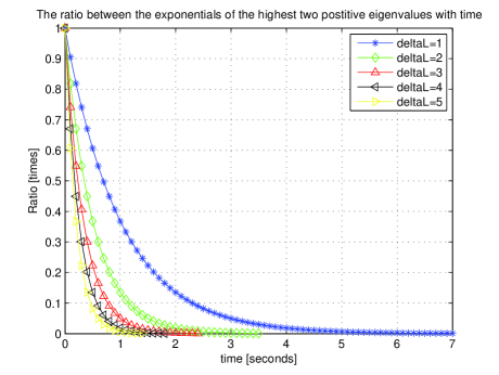
    In eq.(62), because Δλ>0Δ𝜆0\Delta\lambda>0 is a finite number, the K(t)𝐾𝑡K(t) exponentially vanishes (approaches to zero), as will be depicted in Fig. 1, and there exists a finite time constant tT2subscript𝑡subscript𝑇2t_{T_{2}} for a given small positive number ϵ2>0subscriptitalic-ϵ20\epsilon_{2}>0 such that

    |K(ttT2)|<ϵ2𝐾𝑡subscript𝑡subscript𝑇2subscriptitalic-ϵ2|K(t\geq t_{T_{2}})|<\epsilon_{2} (63)

    Similarly, for the denominator terms, we define the following ratio

    λje(λjr)tλmaxe(r+λmax)t=K(t)(1Δλλj+Δλ)<K(t)subscript𝜆𝑗superscript𝑒subscript𝜆𝑗𝑟𝑡subscript𝜆𝑚𝑎𝑥superscript𝑒𝑟subscript𝜆𝑚𝑎𝑥𝑡𝐾𝑡1Δ𝜆subscript𝜆𝑗Δ𝜆𝐾𝑡\displaystyle\frac{\lambda_{j}e^{(\lambda_{j}-r)t}}{\lambda_{max}e^{(-r+\lambda_{max})t}}=K(t)(1-\frac{\Delta\lambda}{\lambda_{j}+\Delta\lambda})<K(t) (64)
    Δλ,λj>0Δ𝜆subscript𝜆𝑗0\displaystyle\quad\quad\Delta\lambda,\lambda_{j}>0
    Refer to caption
    Figure 1: The figure shows the ratio K𝐾K in eq.(61) for some different ΔλΔ𝜆\Delta\lambda values.

    So, the K(t)𝐾𝑡K(t) in eq.(61) is obtained as a multiplier in the ratio of the two greatest terms of the sum in both nominator and denominator. We plot the ratio K(t)𝐾𝑡K(t) in Fig. 1 for some different ΔλΔ𝜆\Delta\lambda values. The Figure 1 shows that the term related to the λmaxsubscript𝜆𝑚𝑎𝑥\lambda_{max} dominates the sum of the nominator and that of the denominator respectively. This observation implies from eq.(59) that

    xisp(t)Jsp,i(t)superscriptsubscript𝑥𝑖𝑠𝑝𝑡subscript𝐽𝑠𝑝𝑖𝑡\displaystyle\frac{x_{i}^{sp}(t)}{J_{sp,i}(t)} =\displaystyle= jsSe(r+λjs)t𝐮js(i)jsSλjse(r+λjs)t𝐮js(i)subscript𝑗𝑠𝑆superscript𝑒𝑟subscript𝜆subscript𝑗𝑠𝑡subscript𝐮subscript𝑗𝑠𝑖subscript𝑗𝑠𝑆subscript𝜆subscript𝑗𝑠superscript𝑒𝑟subscript𝜆subscript𝑗𝑠𝑡subscript𝐮subscript𝑗𝑠𝑖\displaystyle\frac{\sum_{js\in S}e^{(-r+\lambda_{j_{s}})t}{\bf u}_{j_{s}}(i)}{\sum_{js\in S}\lambda_{j_{s}}e^{(-r+\lambda_{j_{s}})t}{\bf u}_{j_{s}}(i)} (65)
    \displaystyle\rightarrow e(r+λmax)tλmaxe(r+λmax)t=1λmaxsuperscript𝑒𝑟subscript𝜆𝑚𝑎𝑥𝑡subscript𝜆𝑚𝑎𝑥superscript𝑒𝑟subscript𝜆𝑚𝑎𝑥𝑡1subscript𝜆𝑚𝑎𝑥\displaystyle\frac{e^{(-r+\lambda_{max})t}}{\lambda_{max}e^{(-r+\lambda_{max})t}}=\frac{1}{\lambda_{max}} (66)
  4. 4.

    If the largest positive eigenvalue in case 3 above is a multiple eigenvale, then, similarly, the corresponding terms in the sum of the nominator and that of the demoninator become dominant, which implies from eq.(59) that xisp(t)Ji(t)superscriptsubscript𝑥𝑖𝑠𝑝𝑡subscript𝐽𝑖𝑡\frac{x_{i}^{sp}(t)}{J_{i}(t)} exponentially converges to 1λmax1subscript𝜆𝑚𝑎𝑥\frac{1}{\lambda_{max}} as time evolves.

Using the observations 1 to 4, and the ”SIR” definition in eq.(2), we conclude from eq.(58), (65) and (66) that for any initial vector 𝐱(0)𝐱0{\bf x}(0) which is not completely perpendicular to the eigenvector corresponding to the largest eigenvalue of 𝐖𝐖{\bf W},

θi(t)=rxisp(t)Jsp,i(t)rλmax,i=1,,N,formulae-sequencesubscript𝜃𝑖𝑡𝑟superscriptsubscript𝑥𝑖𝑠𝑝𝑡subscript𝐽𝑠𝑝𝑖𝑡𝑟subscript𝜆𝑚𝑎𝑥𝑖1𝑁{\theta_{i}}(t\rightarrow\infty)=\frac{rx_{i}^{sp}(t)}{J_{sp,i}(t)}\rightarrow\frac{r}{\lambda_{max}},\quad i=1,\dots,N, (67)

which completes the first part of the proof. Furthermore, from eq. (52), (63) and (67) we conclude that there exists a finite time constant tTsubscript𝑡𝑇t_{T} for a given small positive number ϵc>0subscriptitalic-ϵ𝑐0\epsilon_{c}>0 such that

|θvec(ttT)θult,vec|ϵcsuperscript𝜃𝑣𝑒𝑐𝑡subscript𝑡𝑇superscript𝜃𝑢𝑙𝑡𝑣𝑒𝑐subscriptitalic-ϵ𝑐|{\bf\theta}^{vec}(t\geq t_{T})-{\bf\theta}^{ult,vec}|\leq\epsilon_{c} (68)

where θvec(t)=[θ1(t)θN(t)]Tsuperscript𝜃𝑣𝑒𝑐𝑡superscriptdelimited-[]subscript𝜃1𝑡subscript𝜃𝑁𝑡𝑇{\bf\theta}^{vec}(t)=[\theta_{1}(t)\dots\theta_{N}(t)]^{T} and θult,vec=θult[11]Tsuperscript𝜃𝑢𝑙𝑡𝑣𝑒𝑐superscript𝜃𝑢𝑙𝑡superscriptdelimited-[]11𝑇{\bf\theta}^{ult,vec}=\theta^{ult}[1\dots 1]^{T}, which completes the proof.

Definition: System-Specific Ultimate SIR value: In proposition 1, we showed that the SIR in (2) for every state in the autonomous linear dynamic networks in eq.(4) converges to a constant value as time goes to infinity. We call this converged constant value as ”system specific ultimate SIR” and denote as θultsuperscript𝜃𝑢𝑙𝑡{\theta}^{ult}:

θult=rλmaxsuperscript𝜃𝑢𝑙𝑡𝑟subscript𝜆𝑚𝑎𝑥{\theta}^{ult}=\frac{r}{\lambda_{max}} (69)

where r>0𝑟0r>0 is the design parameter and λmaxsubscript𝜆𝑚𝑎𝑥\lambda_{max} is the maximum (positive) eigenvalue of matrix 𝐖𝐖{\bf W}.

II-B Discrete-time Analysis

In this subsection, we analyse the defined “SIR” for the the underlying linear part of the proposed discrete-time autonomous network which is obtained by discretizing the continuous-time system of eq.(4) by using well-known Euler method:

𝐱(k+1)=(𝐈+α(r𝐈+𝐖))𝐱(k)𝐱𝑘1𝐈𝛼𝑟𝐈𝐖𝐱𝑘{\mathbf{x}}(k+1)=\big{(}{\bf I}+\alpha(-r{\bf I}+{\bf W})\big{)}{\mathbf{x}}(k) (70)

where 𝐈𝐈{\bf I} is the identity matrix, r𝑟r is a positive real number, r𝐈𝑟𝐈-r{\bf I} and 𝐖𝐖{\bf W} is as eq.(14), 𝐱(k)𝐱𝑘{\mathbf{x}}(k) shows the state vector at step k𝑘k, and α>0𝛼0\alpha>0 is the step size.

Proposition 2:

In the autonomous discrete-time linear network of eq.(70), let’s assume that the spectral radius of the system matrix (𝐈+α(r𝐈+𝐖))𝐈𝛼𝑟𝐈𝐖\big{(}{\bf I}+\alpha(-r{\bf I}+{\bf W})\big{)} is larger than 1. (This assumption is equal to the assumption that 𝐖𝐖{\bf W} has positive eigenvalue(s) and r>0𝑟0r>0 is chosen such that λmax>rsubscript𝜆𝑚𝑎𝑥𝑟\lambda_{max}>r, where λmaxsubscript𝜆𝑚𝑎𝑥\lambda_{max} is the maximum (positive) eigenvalue of 𝐖𝐖{\bf W}). If α𝛼\alpha is chosen such that 0<αr<10𝛼𝑟10<\alpha r<1, then

  1. 1.

    the defined ”SIR” θi(k)subscript𝜃𝑖𝑘{\theta_{i}}(k) in eq.(2) for any state i𝑖i asymptotically converges to the “ultimate SIR” constant in (15) as time step evolves for any initial vector 𝐱(0)𝐱0{\bf x}(0) which is not completely perpendicular to the eigenvector corresponding to the largest eigenvalue of 𝐖𝐖{\bf W}.

  2. 2.

    there exists a finite step number kTsubscript𝑘𝑇k_{T} for a given small positive number ϵd>0subscriptitalic-ϵ𝑑0\epsilon_{d}>0 such that

    θvec(kkT)θult,vec<ϵdnormsuperscript𝜃𝑣𝑒𝑐𝑘subscript𝑘𝑇superscript𝜃𝑢𝑙𝑡𝑣𝑒𝑐subscriptitalic-ϵ𝑑||{\bf\theta}^{vec}(k\geq k_{T})-{\bf\theta}^{ult,vec}||<\epsilon_{d} (71)

    where θvec(k)=[θ1(k)θN(k)]Tsuperscript𝜃𝑣𝑒𝑐𝑘superscriptdelimited-[]subscript𝜃1𝑘subscript𝜃𝑁𝑘𝑇{\bf\theta}^{vec}(k)=[\theta_{1}(k)\dots\theta_{N}(k)]^{T} and θult,vec=θult[11]Tsuperscript𝜃𝑢𝑙𝑡𝑣𝑒𝑐superscript𝜃𝑢𝑙𝑡superscriptdelimited-[]11𝑇{\bf\theta}^{ult,vec}=\theta^{ult}[1\dots 1]^{T}.

Proof:

From eq. (70), it’s obtained

𝐱(k)=(𝐈+α(r𝐈+𝐖))k𝐱(0)𝐱𝑘superscript𝐈𝛼𝑟𝐈𝐖𝑘𝐱0{\mathbf{x}}(k)=\Big{(}{\bf I}+\alpha(-r{\bf I}+{\bf W})\Big{)}^{k}{\mathbf{x}}(0) (72)

where 𝐱(0)𝐱0{\bf x}(0) shows the initial state vector at step zero. Let us first examine the powers of the matrix (𝐈+α(r𝐈+𝐖))𝐈𝛼𝑟𝐈𝐖\Big{(}{\bf I}+\alpha(-r{\bf I}+{\bf W})\Big{)} in (72) in terms of matrix r𝐈𝑟𝐈r{\bf I} and the eigenvectors of matrix 𝐖𝐖{\bf W}: It’s well known that any symmetric real square matrix can be decomposed into

𝐖=i=1Nλi𝐯i𝐯iT=i=1Nλi𝐕i𝐖superscriptsubscript𝑖1𝑁subscript𝜆𝑖subscript𝐯𝑖superscriptsubscript𝐯𝑖𝑇superscriptsubscript𝑖1𝑁subscript𝜆𝑖subscript𝐕𝑖{\bf W}=\sum_{i=1}^{N}\lambda_{i}{\bf v}_{i}{\bf v}_{i}^{T}=\sum_{i=1}^{N}\lambda_{i}{\bf V}_{i} (73)

where {λi}i=1Nsuperscriptsubscriptsubscript𝜆𝑖𝑖1𝑁\{\lambda_{i}\}_{i=1}^{N} and {𝐯i}i=1Nsuperscriptsubscriptsubscript𝐯𝑖𝑖1𝑁\{{\bf v}_{i}\}_{i=1}^{N} show the (real) eigenvalues and the corresponding eigenvectors and the eigenvectors {𝐯i}i=1Nsuperscriptsubscriptsubscript𝐯𝑖𝑖1𝑁\{{\bf v}_{i}\}_{i=1}^{N} are orthonormal (see e.g. [16]), i.e.,

𝐯iT𝐯j={1,ifi=j,wherei,j=1,2,,N0,ifij,superscriptsubscript𝐯𝑖𝑇subscript𝐯𝑗cases1formulae-sequenceif𝑖𝑗where𝑖𝑗12𝑁0if𝑖𝑗{\bf v}_{i}^{T}{\bf v}_{j}=\left\{\begin{array}[]{ll}1,&\textrm{if}\quad i=j,\quad\quad\textrm{where}\quad i,j=1,2,\dots,N\\ 0,&\textrm{if}\quad i\neq j,\end{array}\right. (74)

Let’s define the outer-product matrices of the eigenvectors {λi}i=1Nsuperscriptsubscriptsubscript𝜆𝑖𝑖1𝑁\{\lambda_{i}\}_{i=1}^{N} as 𝐕j=𝐯i𝐯iT,i=1,2,,Nformulae-sequencesubscript𝐕𝑗subscript𝐯𝑖superscriptsubscript𝐯𝑖𝑇𝑖12𝑁{\bf V}_{j}={\bf v}_{i}{\bf v}_{i}^{T},\quad i=1,2,\dots,N; and, furthermore, the matrix 𝐌𝐌{\bf M} as

𝐌=𝐈+α(r𝐈+𝐖)𝐌𝐈𝛼𝑟𝐈𝐖{\bf M}={\bf I}+\alpha(-r{\bf I}+{\bf W}) (75)

which is obtained using eq.(73) as

𝐌=(1αr)𝐈+i=1Nβi(1)𝐕i𝐌1𝛼𝑟𝐈superscriptsubscript𝑖1𝑁subscript𝛽𝑖1subscript𝐕𝑖{\bf M}=(1-\alpha r){\bf I}+\sum_{i=1}^{N}\beta_{i}(1){\bf V}_{i} (76)

where r>0𝑟0r>0, α>0𝛼0\alpha>0, and where βi(1)subscript𝛽𝑖1\beta_{i}(1) is equal to

βi(1)=αλi.subscript𝛽𝑖1𝛼subscript𝜆𝑖\beta_{i}(1)=\alpha\lambda_{i}. (77)

The matrix 𝐌2superscript𝐌2{\bf M}^{2} can be written as

𝐌2=(1αr)2𝐈+i=1Nβi(2)𝐕isuperscript𝐌2superscript1𝛼𝑟2𝐈superscriptsubscript𝑖1𝑁subscript𝛽𝑖2subscript𝐕𝑖{\bf M}^{2}=(1-\alpha r)^{2}{\bf I}+\sum_{i=1}^{N}\beta_{i}(2){\bf V}_{i} (78)

where βi(2)subscript𝛽𝑖2\beta_{i}(2) is equal to

βi(2)=α(1αr)λi+(1αr+αλi)βi(1)subscript𝛽𝑖2𝛼1𝛼𝑟subscript𝜆𝑖1𝛼𝑟𝛼subscript𝜆𝑖subscript𝛽𝑖1\beta_{i}(2)=\alpha(1-\alpha r)\lambda_{i}+(1-\alpha r+\alpha\lambda_{i})\beta_{i}(1) (79)

Similarly, the matrix 𝐌3superscript𝐌3{\bf M}^{3} can be written as

𝐌3=(1αr)3𝐈+i=1Nβi(3)𝐕isuperscript𝐌3superscript1𝛼𝑟3𝐈superscriptsubscript𝑖1𝑁subscript𝛽𝑖3subscript𝐕𝑖{\bf M}^{3}=(1-\alpha r)^{3}{\bf I}+\sum_{i=1}^{N}\beta_{i}(3){\bf V}_{i} (80)

where βi(3)subscript𝛽𝑖3\beta_{i}(3) is equal to

βi(3)=α(1αr)2λi+(1αr+αλi)βi(2)subscript𝛽𝑖3𝛼superscript1𝛼𝑟2subscript𝜆𝑖1𝛼𝑟𝛼subscript𝜆𝑖subscript𝛽𝑖2\beta_{i}(3)=\alpha(1-\alpha r)^{2}\lambda_{i}+(1-\alpha r+\alpha\lambda_{i})\beta_{i}(2) (81)

So, 𝐌4superscript𝐌4{\bf M}^{4} can be written as

𝐌4=(1αr)4𝐈+i=1Nβi(4)𝐕isuperscript𝐌4superscript1𝛼𝑟4𝐈superscriptsubscript𝑖1𝑁subscript𝛽𝑖4subscript𝐕𝑖{\bf M}^{4}=(1-\alpha r)^{4}{\bf I}+\sum_{i=1}^{N}\beta_{i}(4){\bf V}_{i} (82)

where βi(4)subscript𝛽𝑖4\beta_{i}(4) is equal to

βi(4)=α(1αr)3λi+(1αr+αλi)βi(3)subscript𝛽𝑖4𝛼superscript1𝛼𝑟3subscript𝜆𝑖1𝛼𝑟𝛼subscript𝜆𝑖subscript𝛽𝑖3\beta_{i}(4)=\alpha(1-\alpha r)^{3}\lambda_{i}+(1-\alpha r+\alpha\lambda_{i})\beta_{i}(3) (83)

So, at step k𝑘k, the matrix (𝐌)ksuperscript𝐌𝑘({\bf M})^{k} is obtained as

𝐌k=(1αr)k𝐈+i=1Nβi(k)𝐕isuperscript𝐌𝑘superscript1𝛼𝑟𝑘𝐈superscriptsubscript𝑖1𝑁subscript𝛽𝑖𝑘subscript𝐕𝑖{\bf M}^{k}=(1-\alpha r)^{k}{\bf I}+\sum_{i=1}^{N}\beta_{i}(k){\bf V}_{i} (84)

where βi(k)subscript𝛽𝑖𝑘\beta_{i}(k) is equal to

βi(k)=α(1αr)k1λi+(1+α(λir))βi(k1)subscript𝛽𝑖𝑘𝛼superscript1𝛼𝑟𝑘1subscript𝜆𝑖1𝛼subscript𝜆𝑖𝑟subscript𝛽𝑖𝑘1\beta_{i}(k)=\alpha(1-\alpha r)^{k-1}\lambda_{i}+(1+\alpha(\lambda_{i}-r))\beta_{i}(k-1) (85)

Using eq.(77) and (85), the βi(k)subscript𝛽𝑖𝑘\beta_{i}(k) is obtained as

βi(1)subscript𝛽𝑖1\displaystyle\beta_{i}(1) =\displaystyle= αλi𝛼subscript𝜆𝑖\displaystyle\alpha\lambda_{i} (86)
βi(2)subscript𝛽𝑖2\displaystyle\beta_{i}(2) =\displaystyle= αλi((1αr)+(1+α(λir)))𝛼subscript𝜆𝑖1𝛼𝑟1𝛼subscript𝜆𝑖𝑟\displaystyle\alpha\lambda_{i}\Big{(}(1-\alpha r)+\big{(}1+\alpha(\lambda_{i}-r)\big{)}\Big{)} (87)
βi(3)subscript𝛽𝑖3\displaystyle\beta_{i}(3) =\displaystyle= αλi((1αr)2+(1αr)(1+α(λir))\displaystyle\alpha\lambda_{i}\Big{(}(1-\alpha r)^{2}+(1-\alpha r)\big{(}1+\alpha(\lambda_{i}-r)\big{)}
+(1+α(λir))2)\displaystyle+\big{(}1+\alpha(\lambda_{i}-r)\big{)}^{2}\Big{)}
\displaystyle\vdots
βi(k)subscript𝛽𝑖𝑘\displaystyle\beta_{i}(k) =\displaystyle= αλim=1k(1αr)km(1+α(λir))m1𝛼subscript𝜆𝑖superscriptsubscript𝑚1𝑘superscript1𝛼𝑟𝑘𝑚superscript1𝛼subscript𝜆𝑖𝑟𝑚1\displaystyle\alpha\lambda_{i}\sum_{m=1}^{k}(1-\alpha r)^{k-m}\big{(}1+\alpha(\lambda_{i}-r)\big{)}^{m-1} (89)

Defining λi=ζi(1αr)subscript𝜆𝑖subscript𝜁𝑖1𝛼𝑟\lambda_{i}=\zeta_{i}(1-\alpha r), we obtain

(1αr)km(1+α(λir))m1=(1αr)k1(1+αζi)m1superscript1𝛼𝑟𝑘𝑚superscript1𝛼subscript𝜆𝑖𝑟𝑚1superscript1𝛼𝑟𝑘1superscript1𝛼subscript𝜁𝑖𝑚1(1-\alpha r)^{k-m}\big{(}1+\alpha(\lambda_{i}-r)\big{)}^{m-1}=(1-\alpha r)^{k-1}(1+\alpha\zeta_{i})^{m-1} (90)

Writing eq.(90) in eq.(89) gives

βi(k)=αζi(1αr)kS(k)subscript𝛽𝑖𝑘𝛼subscript𝜁𝑖superscript1𝛼𝑟𝑘𝑆𝑘\beta_{i}(k)=\alpha\zeta_{i}(1-\alpha r)^{k}S(k) (91)

where S(k)𝑆𝑘S(k) is

S(k)=m=1k(1+αζi)m1𝑆𝑘superscriptsubscript𝑚1𝑘superscript1𝛼subscript𝜁𝑖𝑚1S(k)=\sum_{m=1}^{k}(1+\alpha\zeta_{i})^{m-1} (92)

Summing S(k)𝑆𝑘-S(k) with (1+αζi)S(k)1𝛼subscript𝜁𝑖𝑆𝑘(1+\alpha\zeta_{i})S(k) yields

S(k)=(1+αζi)k1αζi𝑆𝑘superscript1𝛼subscript𝜁𝑖𝑘1𝛼subscript𝜁𝑖S(k)=\frac{(1+\alpha\zeta_{i})^{k}-1}{\alpha\zeta_{i}} (93)

From eq.(91), (92) and (93), we obtain

βi(k)=(1αr)k(1+αζi)k(1αr)ksubscript𝛽𝑖𝑘superscript1𝛼𝑟𝑘superscript1𝛼subscript𝜁𝑖𝑘superscript1𝛼𝑟𝑘\beta_{i}(k)=(1-\alpha r)^{k}(1+\alpha\zeta_{i})^{k}-(1-\alpha r)^{k} (94)

Using the definition ζi=λi/(1αr)subscript𝜁𝑖subscript𝜆𝑖1𝛼𝑟\zeta_{i}=\lambda_{i}/(1-\alpha r) in eq.(94) gives

βi(k)=(1+α(λir))k(1αr)ksubscript𝛽𝑖𝑘superscript1𝛼subscript𝜆𝑖𝑟𝑘superscript1𝛼𝑟𝑘\beta_{i}(k)=\big{(}1+\alpha(\lambda_{i}-r)\big{)}^{k}-(1-\alpha r)^{k} (95)

From eq.(84) and eq.(95),

𝐌k=(1αr)k𝐈+i=1N(1+α(λir))k𝐕ii=1N(1αr)k𝐕isuperscript𝐌𝑘superscript1𝛼𝑟𝑘𝐈superscriptsubscript𝑖1𝑁superscript1𝛼subscript𝜆𝑖𝑟𝑘subscript𝐕𝑖superscriptsubscript𝑖1𝑁superscript1𝛼𝑟𝑘subscript𝐕𝑖{\bf M}^{k}=(1-\alpha r)^{k}{\bf I}+\sum_{i=1}^{N}\big{(}1+\alpha(\lambda_{i}-r)\big{)}^{k}{\bf V}_{i}-\sum_{i=1}^{N}(1-\alpha r)^{k}{\bf V}_{i} (96)

Let’s put the N𝑁N eigenvalues of matrix 𝐖𝐖{\bf W} into two groups as follows: Let those eigenvalues which are smaller that r𝑟r, belong to set T={λjt}jt=1Nt𝑇superscriptsubscriptsubscript𝜆subscript𝑗𝑡subscript𝑗𝑡1subscript𝑁𝑡T=\{\lambda_{j_{t}}\}_{j_{t}=1}^{N_{t}} where Ntsubscript𝑁𝑡N_{t} is the length of the set; and let those eigenvalues which are larger than r𝑟r belong to set S={λjs}js=1Ns𝑆superscriptsubscriptsubscript𝜆subscript𝑗𝑠subscript𝑗𝑠1subscript𝑁𝑠S=\{\lambda_{j_{s}}\}_{j_{s}=1}^{N_{s}} where Nssubscript𝑁𝑠N_{s} is the length of the set. We write the matrix 𝐌ksuperscript𝐌𝑘{\bf M}^{k} in eq.(96) using this eigenvalue grouping

𝐌k=𝐌tp(k)+𝐌sp(k)superscript𝐌𝑘subscript𝐌𝑡𝑝𝑘subscript𝐌𝑠𝑝𝑘{\mathbf{M}}^{k}={\bf M}_{tp}(k)+{\bf M}_{sp}(k) (97)

where

𝐌tp(k)subscript𝐌𝑡𝑝𝑘\displaystyle{\bf M}_{tp}(k) =\displaystyle= (1αr)k𝐈i=1N(1αr)k𝐕isuperscript1𝛼𝑟𝑘𝐈superscriptsubscript𝑖1𝑁superscript1𝛼𝑟𝑘subscript𝐕𝑖\displaystyle(1-\alpha r)^{k}{\bf I}-\sum_{i=1}^{N}(1-\alpha r)^{k}{\bf V}_{i} (98)
+jtT(1+α(λjtr))k𝐕jtsubscriptsubscript𝑗𝑡𝑇superscript1𝛼subscript𝜆subscript𝑗𝑡𝑟𝑘subscript𝐕subscript𝑗𝑡\displaystyle+\sum_{j_{t}\in T}\big{(}1+\alpha(\lambda_{j_{t}}-r)\big{)}^{k}{\bf V}_{j_{t}}

and

𝐌sp(k)=jsS(1+α(λjsr))k𝐕jssubscript𝐌𝑠𝑝𝑘subscriptsubscript𝑗𝑠𝑆superscript1𝛼subscript𝜆subscript𝑗𝑠𝑟𝑘subscript𝐕subscript𝑗𝑠{\bf M}_{sp}(k)=\sum_{j_{s}\in S}\big{(}1+\alpha(\lambda_{j_{s}}-r)\big{)}^{k}{\bf V}_{j_{s}} (99)

We call the matrices 𝐌tp(k)subscript𝐌𝑡𝑝𝑘{\bf M}_{tp}(k) and 𝐌sp(k)subscript𝐌𝑠𝑝𝑘{\bf M}_{sp}(k) in (98) and (99) as transitory phase part and steady phase part, respectively, of the matrix 𝐌ksuperscript𝐌𝑘{\mathbf{M}}^{k}.

It’s observed from eq.(98) that the 𝐌tp(k)subscript𝐌𝑡𝑝𝑘{\bf M}_{tp}(k) converges to zero matrix as time step number evolves because relatively small step number α>0𝛼0\alpha>0 is chosen such that (1αr)<11𝛼𝑟1(1-\alpha r)<1 and 1+α(λjtr)<11𝛼subscript𝜆subscript𝑗𝑡𝑟11+\alpha(\lambda_{j_{t}}-r)<1. Therefore, there exists a finite time step number kT1subscript𝑘subscript𝑇1k_{T_{1}} for a given small positive number ϵ3>0subscriptitalic-ϵ30\epsilon_{3}>0 such that

𝐌tp(kkT1)<ϵ3normsubscript𝐌𝑡𝑝𝑘subscript𝑘subscript𝑇1subscriptitalic-ϵ3||{\bf M}_{tp}(k\geq k_{T_{1}})||<\epsilon_{3} (100)

Thus, (from eq.(75) and (97)), what shapes the steady state behavior of the system in eq.(72) is merely the 𝐌sp(k)subscript𝐌𝑠𝑝𝑘{\bf M}_{sp}(k) in eq.(99 ). So, the steady phase solution is obtained from eqs.(72), (75) and (97)-(99) using the above observations as follows

𝐱sp(k)subscript𝐱𝑠𝑝𝑘\displaystyle{\bf x}_{sp}(k) =\displaystyle= 𝐌sp(k)𝐱(0)subscript𝐌𝑠𝑝𝑘𝐱0\displaystyle{\bf M}_{sp}(k){\bf x}(0) (101)
=\displaystyle= jsS(1+α(λjsr))k𝐕js𝐱(0)subscriptsubscript𝑗𝑠𝑆superscript1𝛼subscript𝜆subscript𝑗𝑠𝑟𝑘subscript𝐕subscript𝑗𝑠𝐱0\displaystyle\sum_{j_{s}\in S}\big{(}1+\alpha(\lambda_{j_{s}}-r)\big{)}^{k}{\bf V}_{j_{s}}{\bf x}(0) (102)

Let’s define the interference vector, 𝐉sp(k)subscript𝐉𝑠𝑝𝑘{\bf J}_{sp}(k) as

𝐉sp(k)=𝐖𝐱sp(k)subscript𝐉𝑠𝑝𝑘subscript𝐖𝐱𝑠𝑝𝑘{\bf J}_{sp}(k)={\bf W}{\bf x}_{sp}(k) (103)

Using eq.(73) in (103) and the orthonormal features in (74) yields

𝐉sp(k)=jsSλjs(1+α(λjsr))k𝐕js𝐱(0)subscript𝐉𝑠𝑝𝑘subscriptsubscript𝑗𝑠𝑆subscript𝜆subscript𝑗𝑠superscript1𝛼subscript𝜆subscript𝑗𝑠𝑟𝑘subscript𝐕subscript𝑗𝑠𝐱0{\bf J}_{sp}(k)=\sum_{j_{s}\in S}\lambda_{j_{s}}\big{(}1+\alpha(\lambda_{j_{s}}-r)\big{)}^{k}{\bf V}_{j_{s}}{\bf x}(0) (104)

First defining 𝐕j𝐱(0)=𝐮jsubscript𝐕𝑗𝐱0subscript𝐮𝑗{\bf V}_{j}{\bf x}(0)={\bf u}_{j}, and ξ=α1αr𝜉𝛼1𝛼𝑟\xi=\frac{\alpha}{1-\alpha r}, then dividing vector 𝐱sp(k)subscript𝐱𝑠𝑝𝑘{\bf x}_{sp}(k) of eq.(102) to 𝐉sp(k)subscript𝐉𝑠𝑝𝑘{\bf J}_{sp}(k) of eq.(104) elementwise and comparing the outcome with the ”SIR” definition in eq.(2) results in

xsp,i(k)Jsp,i(k)subscript𝑥𝑠𝑝𝑖𝑘subscript𝐽𝑠𝑝𝑖𝑘\displaystyle\frac{x_{sp,i}(k)}{J_{sp,i}(k)} =\displaystyle= 1rθi(k),i=1,,Nformulae-sequence1𝑟subscript𝜃𝑖𝑘𝑖1𝑁\displaystyle\frac{1}{r}{\theta_{i}}(k),\quad\quad\quad\quad\quad i=1,\dots,N (105)
=\displaystyle= jsS(1+ξλjs)kujs,ijsSλjs(1+ξλjs)kujs,isubscriptsubscript𝑗𝑠𝑆superscript1𝜉subscript𝜆subscript𝑗𝑠𝑘subscript𝑢subscript𝑗𝑠𝑖subscriptsubscript𝑗𝑠𝑆subscript𝜆subscript𝑗𝑠superscript1𝜉subscript𝜆subscript𝑗𝑠𝑘subscript𝑢subscript𝑗𝑠𝑖\displaystyle\frac{\sum_{j_{s}\in S}(1+\xi\lambda_{j_{s}})^{k}u_{j_{s},i}}{\sum_{j_{s}\in S}\lambda_{j_{s}}(1+\xi\lambda_{j_{s}})^{k}u_{j_{s},i}} (106)

In eq.(106), we assume that the 𝐮j=𝐕j𝐱(0)subscript𝐮𝑗subscript𝐕𝑗𝐱0{\bf u}_{j}={\bf V}_{j}{\bf x}(0) which corresponds to the eigenvector of the largest positive eigenvalue is different than zero vector. This means that we assume in the analysis here that 𝐱(0)𝐱0{\bf x}(0) is not completely perpendicular to the mentioned eigenvector.

From the analysis above, we observe that

  1. 1.

    If there is only one positive eigenvalue which is greater than r𝑟r and it’s a multiple one, denoted as λbsubscript𝜆𝑏\lambda_{b}, then it’s seen from (106) that

    θi(k)=rλb,k,i=1,,Nformulae-sequencesubscript𝜃𝑖𝑘𝑟subscript𝜆𝑏formulae-sequence𝑘𝑖1𝑁\displaystyle{\theta_{i}}(k)=\frac{r}{\lambda_{b}},\quad k\rightarrow\infty,\quad i=1,\dots,N (107)
  2. 2.

    Similarly, if there is only one positive eigenvalue which is larger than r𝑟r and it’s a single one, shown as λbsubscript𝜆𝑏\lambda_{b}, then eq.(107) holds.

  3. 3.

    If there are more than two different (positive) eigenvalues and the largest positive eigenvalue is single (not multiple), then we see from (105) that the term related to the largest (positive) eigenvalue dominates the sum of the nominator. Same observation is valid for the sum of the denominator. This is because a relatively small increase in λjsubscript𝜆𝑗\lambda_{j} causes exponential increase as time step evolves, which is shown in the following: Let’s show the two largest (positive) eigenvalues as λmaxsubscript𝜆𝑚𝑎𝑥\lambda_{max} and λjsubscript𝜆𝑗\lambda_{j} respectively and the difference between them as ΔλΔ𝜆\Delta\lambda. So, λmax=λj+Δλsubscript𝜆𝑚𝑎𝑥subscript𝜆𝑗Δ𝜆\lambda_{max}=\lambda_{j}+\Delta\lambda. Let’s define the following ratio between the terms related to the two highest eigenvalues in the nominator

    Kn(k)=(1+ξλj)k(1+ξ(λj+Δλ))ksubscript𝐾𝑛𝑘superscript1𝜉subscript𝜆𝑗𝑘superscript1𝜉subscript𝜆𝑗Δ𝜆𝑘K_{n}(k)=\frac{(1+\xi\lambda_{j})^{k}}{(1+\xi(\lambda_{j}+\Delta\lambda))^{k}} (108)

    where

    ξ=α1αr.𝜉𝛼1𝛼𝑟\xi=\frac{\alpha}{1-\alpha r}. (109)

    In eq.(108), because Δλ>0Δ𝜆0\Delta\lambda>0, there exists a finite time step number kT2subscript𝑘subscript𝑇2k_{T_{2}} for a given small positive number ϵ3>0subscriptitalic-ϵ30\epsilon_{3}>0 such that

    |Kn(k)|<ϵ3subscript𝐾𝑛𝑘subscriptitalic-ϵ3|K_{n}(k)|<\epsilon_{3} (110)

    Similarly, let’s define the ratio between the terms related to the two highest eigenvalues in the denominator as

    Kd(k)=λj(1+ξλj)k(λj+Δλ)(1+ξ(λj+Δλ))ksubscript𝐾𝑑𝑘subscript𝜆𝑗superscript1𝜉subscript𝜆𝑗𝑘subscript𝜆𝑗Δ𝜆superscript1𝜉subscript𝜆𝑗Δ𝜆𝑘K_{d}(k)=\frac{\lambda_{j}(1+\xi\lambda_{j})^{k}}{(\lambda_{j}+\Delta\lambda)(1+\xi(\lambda_{j}+\Delta\lambda))^{k}} (111)

    From eq.(108) and (111), because Δλ>0Δ𝜆0\Delta\lambda>0 and λjλj+Δλ<1subscript𝜆𝑗subscript𝜆𝑗Δ𝜆1\frac{\lambda_{j}}{\lambda_{j}+\Delta\lambda}<1,

    Kd(k)<Kn(k).subscript𝐾𝑑𝑘subscript𝐾𝑛𝑘K_{d}(k)<K_{n}(k). (112)

    and there exists a finite time step number kT2subscript𝑘subscript𝑇2k_{T_{2}} for a given small positive number ϵ4>0subscriptitalic-ϵ40\epsilon_{4}>0 such that

    |Kn(kkT2)|<ϵ4.subscript𝐾𝑛𝑘subscript𝑘subscript𝑇2subscriptitalic-ϵ4|K_{n}(k\geq k_{T_{2}})|<\epsilon_{4}. (113)
    Refer to caption
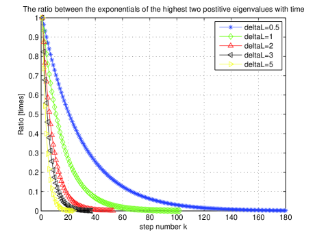
    Figure 2: The figure shows the ratio Knsubscript𝐾𝑛K_{n} in eq.(108) for some different ΔλΔ𝜆\Delta\lambda values (λ=5,ξ=0.11formulae-sequence𝜆5𝜉0.11\lambda=5,\xi=0.11).

    We plot the ratio Kn(k)subscript𝐾𝑛𝑘K_{n}(k) in Fig. 2 for some different ΔλΔ𝜆\Delta\lambda values and for a typical ξ𝜉\xi value. The Figure 2 and eq.(112) implies that the terms related to the λmaxsubscript𝜆𝑚𝑎𝑥\lambda_{max} dominate the sum of the nominator and that of the denominator respectively. So, from eq.(106) and (109),

    xsp,i(k)Jsp,i(k)subscript𝑥𝑠𝑝𝑖𝑘subscript𝐽𝑠𝑝𝑖𝑘\displaystyle\frac{x_{sp,i}(k)}{J_{sp,i}(k)} =\displaystyle= jsS(1+ξλjs)kujs,ijsSλjs(1+ξλjs)kujs,isubscriptsubscript𝑗𝑠𝑆superscript1𝜉subscript𝜆subscript𝑗𝑠𝑘subscript𝑢subscript𝑗𝑠𝑖subscriptsubscript𝑗𝑠𝑆subscript𝜆subscript𝑗𝑠superscript1𝜉subscript𝜆subscript𝑗𝑠𝑘subscript𝑢subscript𝑗𝑠𝑖\displaystyle\frac{\sum_{j_{s}\in S}(1+\xi\lambda_{j_{s}})^{k}u_{j_{s},i}}{\sum_{j_{s}\in S}\lambda_{j_{s}}(1+\xi\lambda_{j_{s}})^{k}u_{j_{s},i}} (114)
    \displaystyle\rightarrow (1+ξλmax)kλmax(1+ξλmax)k=1λmax,superscript1𝜉subscript𝜆𝑚𝑎𝑥𝑘subscript𝜆𝑚𝑎𝑥superscript1𝜉subscript𝜆𝑚𝑎𝑥𝑘1subscript𝜆𝑚𝑎𝑥\displaystyle\frac{(1+\xi\lambda_{max})^{k}}{\lambda_{max}(1+\xi\lambda_{max})^{k}}=\frac{1}{\lambda_{max}},
  4. 4.

    If the largest positive eigenvalue in case 3 above is a multiple eigenvale, then, similarly, the corresponding terms in the sum of the nominator and that of the demoninator become dominant, which implies from eq.(106), (108) and (111) that xsp,i(k)Jsp,i(k)subscript𝑥𝑠𝑝𝑖𝑘subscript𝐽𝑠𝑝𝑖𝑘\frac{x_{sp,i}(k)}{J_{sp,i}(k)} converges to 1λmax1subscript𝜆𝑚𝑎𝑥\frac{1}{\lambda_{max}} as step number increases.

Using the observations 1 to 4, eq.(100), the ”SIR” definition in eq.(2), eq.(105) and (106), we conclude that

θi(k)=rxsp,i(k)Jsp,i(k)rλmaxsubscript𝜃𝑖𝑘𝑟subscript𝑥𝑠𝑝𝑖𝑘subscript𝐽𝑠𝑝𝑖𝑘𝑟subscript𝜆𝑚𝑎𝑥{\theta_{i}}(k\rightarrow\infty)=\frac{rx_{sp,i}(k)}{J_{sp,i}(k)}\rightarrow\frac{r}{\lambda_{max}} (115)

where i=1,,N,𝑖1𝑁i=1,\dots,N, and λmaxsubscript𝜆𝑚𝑎𝑥\lambda_{max} is the largest (positive) eigenvalue of the matrix W, which completes the first part of the proof. Furthermore, from eq. (100), (113) and (115), we conclude that there exists a finite time constant kTsubscript𝑘𝑇k_{T} for a given small positive number ϵd>0subscriptitalic-ϵ𝑑0\epsilon_{d}>0 such that

θvec(kkT)θult,vec<ϵdnormsuperscript𝜃𝑣𝑒𝑐𝑘subscript𝑘𝑇superscript𝜃𝑢𝑙𝑡𝑣𝑒𝑐subscriptitalic-ϵ𝑑||{\bf\theta}^{vec}(k\geq k_{T})-{\bf\theta}^{ult,vec}||<\epsilon_{d} (116)

where θvec(k)=[θ1(k)θN(k)]Tsuperscript𝜃𝑣𝑒𝑐𝑘superscriptdelimited-[]subscript𝜃1𝑘subscript𝜃𝑁𝑘𝑇{\bf\theta}^{vec}(k)=[\theta_{1}(k)\dots\theta_{N}(k)]^{T} and θult,vec=θult[11]Tsuperscript𝜃𝑢𝑙𝑡𝑣𝑒𝑐superscript𝜃𝑢𝑙𝑡superscriptdelimited-[]11𝑇{\bf\theta}^{ult,vec}=\theta^{ult}[1\dots 1]^{T}, which completes the proof.

III Stabilized SIR system

Do the results of the ultimate SIR analysis in Section II above have any practical meanings? Our answer is yes. In this section, we propose two Hopfield-like networks in continuous and discrete-time domain respectively where the “system-specific ultimate SIR” is used to stabilize the system.

III-A Continuous-time SALU-”SIR”

Defining the following g(a)𝑔𝑎g(a) function,

g(a)={1if|a|ϵ,0otherwise𝑔𝑎cases1if𝑎italic-ϵ0otherwise\displaystyle g(a)=\left\{\begin{array}[]{ll}1&\textrm{if}\quad|a|\geq\epsilon,\\ 0&\textrm{otherwise}\end{array}\right. (119)

we propose the following dynamic network,

𝐱˙˙𝐱\displaystyle\dot{{\mathbf{x}}} =\displaystyle= (r𝐈+𝐖)𝐱g(θvec(t)θult,vec)𝑟𝐈𝐖𝐱𝑔normsuperscript𝜃𝑣𝑒𝑐𝑡superscript𝜃𝑢𝑙𝑡𝑣𝑒𝑐\displaystyle(-r{\mathbf{I}}+{\mathbf{W}}){\mathbf{x}}g(||{\bf\theta}^{vec}(t)-{\bf\theta}^{ult,vec}||) (120)
𝐲𝐲\displaystyle{\mathbf{y}} =\displaystyle= sign(𝐱)𝑠𝑖𝑔𝑛𝐱\displaystyle sign({\mathbf{x}}) (121)

where θvec(t)=[θ1(t)θN(t)]Tsuperscript𝜃𝑣𝑒𝑐𝑡superscriptdelimited-[]subscript𝜃1𝑡subscript𝜃𝑁𝑡𝑇{\bf\theta}^{vec}(t)=[\theta_{1}(t)\dots\theta_{N}(t)]^{T} and θult,vec=θult[11]Tsuperscript𝜃𝑢𝑙𝑡𝑣𝑒𝑐superscript𝜃𝑢𝑙𝑡superscriptdelimited-[]11𝑇{\bf\theta}^{ult,vec}=\theta^{ult}[1\dots 1]^{T}, and 𝐲𝐲{\mathbf{y}} is the output of the network.

We call the network in eqs.(119)-(121) as Stabilized Autonomous Linear Networks by Ultimate “SIR” (SAL-U”SIR”).
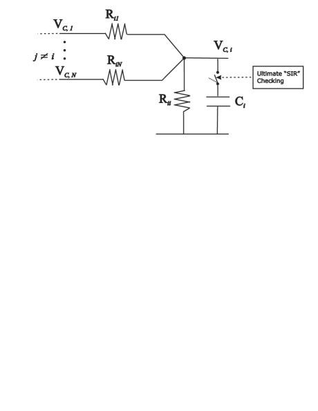
Refer to caption
Figure 3: The figure depicts a sketch of the proposed network for numerical implementation purposes, omitting the considerations on the circuit, called Stabilized Autonomous Linear Networks with Ultimate “SIR” (SAL-U”SIR”).

Proposition 3:

The proposed dynamic network of eqs.(120)-(121) with the weight matrix (r𝐈+𝐖)𝑟𝐈𝐖(-r{\bf I}+{\bf W}) as defined in eq. (14) is stable for any initial condition 𝐱(0)𝐱0{\bf x}(0).

Proof:

If all the eigenvalues of the symmetrix matrix (r𝐈+𝐖)𝑟𝐈𝐖(-r{\bf I}+{\bf W}) as defined in eq. (14) are negative, then it’s well known from linear systems theory that the states go to zero exponentially for any initial vector 𝐱(0)𝐱0{\bf x}(0) (see e.g. [17]).

Otherwise, if there exists positive eigenvalue(s) of (r𝐈+𝐖)𝑟𝐈𝐖(-r{\bf I}+{\bf W}), which is the case in our design, then the proposition 1 above proves for the underlying linear system of (120) that i) the defined SIR in eq.(2) for any state i𝑖i (xi(t),1,2,,N,subscript𝑥𝑖𝑡12𝑁x_{i}(t),\quad 1,2,\dots,N,) converges, as time evolves, to the constant system-specific ultimate SIR value in eq.(15) for any initial vector 𝐱(0)𝐱0{\bf x}(0), and ii) there exists a finite time constant tTsubscript𝑡𝑇t_{T} for a given small positive number ϵ>0italic-ϵ0\epsilon>0 such that θvec(ttT)θult,vec<ϵnormsuperscript𝜃𝑣𝑒𝑐𝑡subscript𝑡𝑇superscript𝜃𝑢𝑙𝑡𝑣𝑒𝑐italic-ϵ||{\bf\theta}^{vec}(t\geq t_{T})-{\bf\theta}^{ult,vec}||<\epsilon. So, the function g()𝑔g(\cdot) stabilizes the system within the tTsubscript𝑡𝑇t_{T} seconds, i.e., once θvec(t)θult,vec<ϵnormsuperscript𝜃𝑣𝑒𝑐𝑡superscript𝜃𝑢𝑙𝑡𝑣𝑒𝑐italic-ϵ||{\bf\theta}^{vec}(t)-{\bf\theta}^{ult,vec}||<\epsilon is met. So, the system is stable.

From the analysis above for symmetric 𝐖𝐖\mathbf{W} and positive r𝐈𝑟𝐈r\mathbf{I}, we observe that

  1. 1.

    The SAL-U”SIR” does not show oscilatory behaviour because all eigenvalues are real (i.e., no imaginary part), and at least one eigenvalue is positive, which is assured by choosing the matrix r𝐈𝑟𝐈r\mathbf{I} accordingly.

  2. 2.

    The transition phase of the ”unstable” linear network is shaped by the initial state vector and the phase space characteristics formed by the eigenvectors. The network is stabilized by the function g()𝑔g(\cdot) once the network has passed the transition phase. The output of the network then is formed taking the sign of the converged states. Whether the state converges to a plus or minus value is dictated by the phase space shaped by the eigenvectors of 𝐖𝐖\mathbf{W} and the initial vector 𝐱(0)𝐱0\mathbf{x}(0).

From observation 1 and 2 above, we see that choosing the positive matrix r𝐈𝑟𝐈r\mathbf{I} such that the matrix (r𝐈+𝐖)𝑟𝐈𝐖(-r{\bf I}+{\bf W}) has positive eigenvalues makes the proposed SAL-U”SIR” exhibit similar features as the Hopfield Network does. The computer simulations in section IV shows the performance of the proposed network as compared to the Hopfield Network in some simple associative memory systems examples.

As far as the possible circuital implementations of the proposed network is concerned, a further research is needed on especially how the nonlinear function g()𝑔g(\cdot) could be implemented on the circuit. In this paper, we mainly focus on the analysis part, and the circuital implementation part is left as a future research topic. However, in order to give an insight, in what follows, we propose the following simplified network for numerical implementation purposes:

It’s well known that a linear dynamic network like (4) can be implemented by RC (Resistance-Capacitance) circuits. Corresponding RC dynamic network is given as follows:

[CV˙C1CV˙C2CV˙CN]=[R11R12R1NR210R2NRN1RN20][VC1VC2VCN]delimited-[]𝐶subscript˙𝑉subscript𝐶1𝐶subscript˙𝑉subscript𝐶2𝐶subscript˙𝑉subscript𝐶𝑁delimited-[]subscript𝑅11subscript𝑅12subscript𝑅1𝑁subscript𝑅210subscript𝑅2𝑁missing-subexpressionsubscript𝑅𝑁1subscript𝑅𝑁20delimited-[]subscript𝑉subscript𝐶1subscript𝑉subscript𝐶2subscript𝑉subscript𝐶𝑁\left[\begin{array}[]{c}C\dot{V}_{C_{1}}\\ C\dot{V}_{C_{2}}\\ \vdots\\ C\dot{V}_{C_{N}}\end{array}\right]=\left[\begin{array}[]{c c c c}R_{11}&R_{12}&\ldots&R_{1N}\\ R_{21}&0&\ldots&R_{2N}\\ \vdots&&\ddots&\vdots\\ R_{N1}&R_{N2}&\ldots&0\end{array}\right]\left[\begin{array}[]{c}V_{C_{1}}\\ V_{C_{2}}\\ \vdots\\ V_{C_{N}}\end{array}\right] (122)

where C𝐶C represents the capacitance, VCisubscript𝑉subscript𝐶𝑖V_{C_{i}} shows the voltage of the capacitance Cisubscript𝐶𝑖C_{i}, which is the state i𝑖i of the network and Rijsubscript𝑅𝑖𝑗R_{ij} is the resistance. From eq.(1), (14) and (122),

Rijsubscript𝑅𝑖𝑗\displaystyle R_{ij} =\displaystyle= 1Cwij,i,j=1,2,,Nandij,formulae-sequence1𝐶subscript𝑤𝑖𝑗𝑖𝑗12𝑁and𝑖𝑗\displaystyle\frac{1}{C}w_{ij},\quad\quad i,j=1,2,\dots,N\quad\textrm{and}\quad i\neq j, (123)
Riisubscript𝑅𝑖𝑖\displaystyle R_{ii} =\displaystyle= r𝑟\displaystyle r (124)

So, we sketch a simplified numerical implementation of the proposed SAL-U”SIR” in Fig. 3, omitting the considerations on circuits, where the function g()𝑔g(\cdot) is represented by a switch (“ultimate SIR checking”).

III-B Discrete-time SALU-”SIR”

The proposed autonomous network in discrete-time, called DSAL-USIR (Discrete Stabilized Autonomous Linear networks by Ultimate “SIR”) is given as follows

𝐱(k+1)𝐱𝑘1\displaystyle{\mathbf{x}}(k+1) =\displaystyle= (𝐈+α(r𝐈+𝐖))𝐱(k)g(θvec(t)θult,vec)𝐈𝛼𝑟𝐈𝐖𝐱𝑘𝑔normsuperscript𝜃𝑣𝑒𝑐𝑡superscript𝜃𝑢𝑙𝑡𝑣𝑒𝑐\displaystyle\Big{(}{\bf I}+\alpha(-r{\bf I}+{\bf W})\Big{)}{\mathbf{x}}(k)g(||{\bf\theta}^{vec}(t)-{\bf\theta}^{ult,vec}||) (125)
𝐲(k)𝐲𝑘\displaystyle{\mathbf{y}}(k) =\displaystyle= sign(𝐱(k))𝑠𝑖𝑔𝑛𝐱𝑘\displaystyle sign({\mathbf{x}}(k)) (126)

where 𝐖𝐖{\bf W} is defined by eq.(14), the function g()𝑔g(\cdot) is defined by eq.(119), α>0𝛼0\alpha>0 is step size, 𝐈𝐈{\bf I} is identity matrix and r>0𝑟0r>0 as in eq.(70), θvec(t)=[θ1(t)θN(t)]Tsuperscript𝜃𝑣𝑒𝑐𝑡superscriptdelimited-[]subscript𝜃1𝑡subscript𝜃𝑁𝑡𝑇{\bf\theta}^{vec}(t)=[\theta_{1}(t)\dots\theta_{N}(t)]^{T} and θult,vec=θult[11]Tsuperscript𝜃𝑢𝑙𝑡𝑣𝑒𝑐superscript𝜃𝑢𝑙𝑡superscriptdelimited-[]11𝑇{\bf\theta}^{ult,vec}=\theta^{ult}[1\dots 1]^{T}, and 𝐲(k)𝐲𝑘{\mathbf{y}}(k) is the output of the network.

Proposition 4:

The proposed discrete-time networks, DSAL-U”SIR”, in eq.(125) and (126) is stable for any initial vector 𝐱(0)𝐱0{\bf x}(0).

Proof:

If the spectral radius of the system matrix (𝐈+α(r𝐈+𝐖))𝐈𝛼𝑟𝐈𝐖\big{(}{\bf I}+\alpha(-r{\bf I}+{\bf W})\big{)} is smaller than 1, then it’s well known from the discrete-time linear systems theory that the states go to zero exponentially for any initial vector 𝐱(0)𝐱0{\bf x}(0) (see e.g. [17]).

If, on the other hand, the spectral radius is larger than 1, which is the case in our design, then the proposition 2 above proves for the underlying linear system (70) that i) the defined “SIR” θi(k)subscript𝜃𝑖𝑘{\theta_{i}}(k) in eq.(2) for any state i𝑖i asymptotically converges to the “system-specific ultimate SIR” constant in (15) as time step evolves for any initial vector 𝐱(0)𝐱0{\bf x}(0) ii) there exists a finite step number kTsubscript𝑘𝑇k_{T} for a given small positive number ϵd>0subscriptitalic-ϵ𝑑0\epsilon_{d}>0 such that θvec(kkT)θult,vec<ϵdnormsuperscript𝜃𝑣𝑒𝑐𝑘subscript𝑘𝑇superscript𝜃𝑢𝑙𝑡𝑣𝑒𝑐subscriptitalic-ϵ𝑑||{\bf\theta}^{vec}(k\geq k_{T})-{\bf\theta}^{ult,vec}||<\epsilon_{d}. So, the function g()𝑔g(\cdot) stabilizes the system within the kTsubscript𝑘𝑇k_{T} steps, i.e., once θvec(t)θult,vec<ϵdnormsuperscript𝜃𝑣𝑒𝑐𝑡superscript𝜃𝑢𝑙𝑡𝑣𝑒𝑐subscriptitalic-ϵ𝑑||{\bf\theta}^{vec}(t)-{\bf\theta}^{ult,vec}||<\epsilon_{d} is met. So, the system is stable.

As far as the design of weight matrix 𝐖𝐖\mathbf{W} and r𝑟r is concerned, we propose to use the following method which is based on the well known Hebb-learning rule [15].

III-C Outer products based network design

Let’s assume that L𝐿L desired prototype vectors, {𝐝s}s=1Lsuperscriptsubscriptsubscript𝐝𝑠𝑠1𝐿\{\mathbf{d}_{s}\}_{s=1}^{L}, are given from (1,+1)Nsuperscript11𝑁(-1,+1)^{N}. The proposed method is based on well-known Hebb-learning [15] as follows:

Step 1: Calculate the sum of outer products of the prototype vectors (Hebb Rule, [15])

𝐐=s=1L𝐝s𝐝sT𝐐superscriptsubscript𝑠1𝐿subscript𝐝𝑠superscriptsubscript𝐝𝑠𝑇\displaystyle\mathbf{Q}=\sum_{s=1}^{L}\mathbf{d}_{s}\mathbf{d}_{s}^{T} (127)

Step 2: Determine the diagonal matrix r𝐈𝑟𝐈r\bf{I} and 𝐖𝐖\bf{W} as follows:

r=qii+ρ𝑟subscript𝑞𝑖𝑖𝜌r=q_{ii}+\rho (128)

where ρ𝜌\rho is a real number and

wij={0ifi=j,qijifiji,j=1,,Nformulae-sequencesubscript𝑤𝑖𝑗cases0if𝑖𝑗subscript𝑞𝑖𝑗if𝑖𝑗𝑖𝑗1𝑁w_{ij}=\left\{\begin{array}[]{ll}0&\textrm{if}\quad i=j,\\ q_{ij}&\textrm{if}\quad i\neq j\end{array}\right.\quad\quad i,j=1,\dots,N (129)

where qijsubscript𝑞𝑖𝑗q_{ij} shows the entries of matrix 𝐐𝐐\mathbf{Q}, N𝑁N is the dimension of the vector 𝐱(t)𝐱𝑡\mathbf{x}(t) and L𝐿L is the number of the prototype vectors (N>L>0𝑁𝐿0N>L>0). From (127), qii=Lsubscript𝑞𝑖𝑖𝐿q_{ii}=L in eq.(128) since {𝐝s}subscript𝐝𝑠\{\mathbf{d}_{s}\} is from (1,+1)Nsuperscript11𝑁(-1,+1)^{N}.

If the desired prototype vectors are orthogonal, then it can be shown, using the steps of the proofs of prepositions 1 and 3 for continuous and discrete-time respectively, that the “system specific ultimate SIR” be θult=rNLsuperscript𝜃𝑢𝑙𝑡𝑟𝑁𝐿\theta^{ult}=\frac{r}{N-L}.

IV Simulation Results

We take the same examples as in [14] for comparison reasons and for the sake of brevity.

In this section, we apply the the proposed networks SAL-U”SIR” and DSAL-U”SIR”, in continuous and discrete-time respectively, to associate memory systems design, and present their simulation results as compared to those of corresponding Hopfield Networks. The weight matrices of the proposed networks and the Hopfield Networks are designed by the outer-products (Hebb learning [15]) learning rule described in Section III-C.

IV-A Continuous-time examples

In this section, we present two examples, one with 8 neurons and one with 16 neurons, in Example 1 and 2 respectively.

The proposed DSALU-SIR network is given by eqs. (120) and (121). The Hopfield Network [1], used as the reference network, is given by

𝐱˙˙𝐱\displaystyle\dot{{\mathbf{x}}} =\displaystyle= r𝐱+𝐖𝐟(𝐱(t))+𝐛𝑟𝐱𝐖𝐟𝐱𝑡𝐛\displaystyle-r{\bf x}+{\bf W}{\mathbf{f}}({\bf x}(t))+{\bf b} (130)
𝐲(t)𝐲𝑡\displaystyle{\mathbf{y}}(t) =\displaystyle= 𝐟(𝐱(t))𝐟𝐱𝑡\displaystyle{\bf f}({\bf x}(t)) (131)

where 𝐖𝐖{\bf W} is the weight matrix and 𝐱(t)𝐱𝑡{\bf x}(t) is the state at time t𝑡t, 𝐛=𝟎𝐛0{\bf b}={\bf 0}, 𝐟(𝐱)=[f(x1)f(x2)f(xN)]T𝐟𝐱superscriptdelimited-[]𝑓subscript𝑥1𝑓subscript𝑥2𝑓subscript𝑥𝑁𝑇{\bf f}({\bf x})=[f(x_{1})f(x_{2})\dots f(x_{N})]^{T}, the f()𝑓f(\cdot) is a sigmoid function, i.e., f(xi)=111+exp(σxi)𝑓subscript𝑥𝑖111𝑒𝑥𝑝𝜎subscript𝑥𝑖f(x_{i})=1-\frac{1}{1+exp(-\sigma x_{i})}, where σ>0𝜎0\sigma>0.

Example 1:

This example is taken from example 1 in [14]. In the design, σ=2𝜎2\sigma=2 and ρ𝜌\rho is chosen as -2, and r=1𝑟1r=1. The desired prototype vectors are given in the raws of matrix 𝐃𝐃{\mathbf{D}} as follows,

𝐃=[111111111111111111111111]𝐃delimited-[]111111111111111111111111{\mathbf{D}}=\left[\begin{array}[]{c c c c c c c c}1&1&1&1&-1&-1&-1&-1\\ 1&1&-1&-1&1&1&-1&-1\\ 1&-1&1&-1&1&-1&1&-1\end{array}\right] (132)

The weight matrix, using the design rule in Section III-C, is obtained as

r𝐈=𝐈,and𝑟𝐈𝐈and\displaystyle r{\mathbf{I}}={\mathbf{I}},\quad\quad\textrm{and}\quad\quad\quad\quad\quad\quad (133)
𝐖=[0111111310111131110113111110311111130111113110111311110131111110],𝐖delimited-[]0111111310111131110113111110311111130111113110111311110131111110\displaystyle{\mathbf{W}}=\left[\begin{array}[]{c c c c c c c c}0&1&1&-1&1&-1&-1&-3\\ 1&0&-1&1&-1&1&-3&-1\\ 1&-1&0&1&-1&-3&1&-1\\ -1&1&1&0&-3&-1&-1&1\\ 1&-1&-1&-3&0&1&1&-1\\ -1&1&-3&-1&1&0&-1&1\\ -1&-3&1&-1&1&-1&0&1\\ -3&-1&-1&1&-1&1&1&0\end{array}\right], (142)

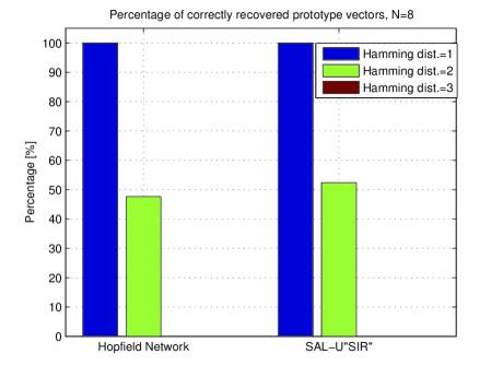
The Figure 4 shows the percentages of correctly recovered desired patterns for all possible initial conditions 𝐱(t=0)(1,+1)N𝐱𝑡0superscript11𝑁\mathbf{x}(t=0)\in(-1,+1)^{N}, in the proposed SALU-”SIR” as compared to traditional Hopfield network.
Refer to caption
Figure 4: The figure shows percentage of correctly recovered desired patterns for all possible initial conditions in example 1 for the proposed SALU-”SIR” as compared to traditional Hopfield network with 8 neurons.

Let mdsubscript𝑚𝑑m_{d} show the number of prototype vectors and C(N,K)𝐶𝑁𝐾C(N,K), (such that NK0𝑁𝐾0N\geq K\geq 0), represent the combination N,K𝑁𝐾N,K, which is equal to C(N,K)=N!(NK)!K!𝐶𝑁𝐾𝑁𝑁𝐾𝐾C(N,K)=\frac{N!}{(N-K)!K!}, where !! shows factorial. In our simulation, the prototype vectors are from (1,1)Nsuperscript11𝑁(-1,1)^{N} as seen above. For initial conditions, we alter the sign of K𝐾K states where K𝐾K=0, 1, 2, 3 and 4, which means the initial condition is within K𝐾K-Hamming distance from the corresponding prototype vector. So, the total number of different possible combinations for the initial conditions for this example is 24, 84 and 168 for 1, 2 and 3-Hamming distance cases respectively, which could be calculated by md×C(8,K)subscript𝑚𝑑𝐶8𝐾m_{d}\times C(8,K), where md=3subscript𝑚𝑑3m_{d}=3 and K=𝐾absentK= 1, 2 and 3.

As seen from Figure 4, the performance of the proposed network SALU”SIR” is the same as that of the continuous Hopfield Network for 1-Hamming distance case (%100\%100 for both networks) and is slightly higher than that of the Hopfield Network for 2 distance case.

Example 2:

This example is taken from example 2 in [14]. The desired prototype vectors as well as the obtained weight matrix 𝐖𝐖{\bf W} are shown in Appendix I. The other network paramaters are chosen as in example 1: σ=2𝜎2\sigma=2 and ρ=2𝜌2\rho=-2 .

The Figure 5 shows the percentages of correctly recovered desired patterns for all possible initial conditions 𝐱(t=0)(1,+1)16𝐱𝑡0superscript1116\mathbf{x}(t=0)\in(-1,+1)^{16}, in the proposed SALU”SIR” as compared to the traditional Hopfield network.
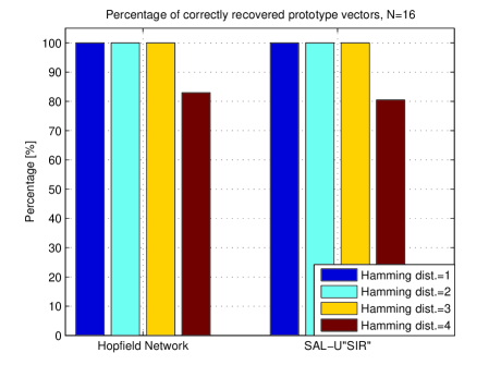
Refer to caption
Figure 5: The figure shows percentage of correctly recovered desired patterns for all possible initial conditions in example 2 for the proposed SALU-”SIR” as compared to traditional Hopfield network with 16 neurons.

The total number of different possible combinations for the initial conditions for this example is 64, 480 and 2240 and 7280 for 1, 2, 3 and 4-Hamming distance cases respectively, which could be calculated by md×C(16,K)subscript𝑚𝑑𝐶16𝐾m_{d}\times C(16,K), where md=4subscript𝑚𝑑4m_{d}=4 and K=𝐾absentK= 1, 2, 3 and 4.

As seen from Figure 5 the performance of the proposed network SALU”SIR” is the same as that of Hopfield Network for 1, 2 and 3-Hamming distance cases (%100\%100 for both networks), and gives comparable performance with the Hopfield Network for 4-Hamming distance case.

IV-B Discrete-time examples

In this section, we present two examples, one with 8 neurons (Example 3) and one with 16 neurons (Example 4). The traditional discrete Hopfield network [1], shown in the following, is used as a reference network:

𝐱k+1=sign(𝐖𝐱k)superscript𝐱𝑘1𝑠𝑖𝑔𝑛superscript𝐖𝐱𝑘{\bf x}^{k+1}=sign\Big{(}{\bf W}{\bf x}^{k}\Big{)} (143)

where 𝐖𝐖{\bf W} is the weight matrix and 𝐱ksuperscript𝐱𝑘{\bf x}^{k} is the state at time k𝑘k, and at most one state is updated at a step.

In the simulations in this subsection, we also examine the following version of the DSAL-U”SIR” for comparison reasons:

𝐱(k+1)𝐱𝑘1\displaystyle{\mathbf{x}}(k+1) =\displaystyle= (ρ𝐈+𝐖)𝐱(k)g(|θvec(t)θult,vec|)𝜌𝐈𝐖𝐱𝑘𝑔superscript𝜃𝑣𝑒𝑐𝑡superscript𝜃𝑢𝑙𝑡𝑣𝑒𝑐\displaystyle(-\rho{\bf I}+{\bf W}){\mathbf{x}}(k)g(|{\bf\theta}^{vec}(t)-{\bf\theta}^{ult,vec}|) (144)
𝐲(k)𝐲𝑘\displaystyle{\mathbf{y}}(k) =\displaystyle= sign(𝐱(k))𝑠𝑖𝑔𝑛𝐱𝑘\displaystyle sign({\mathbf{x}}(k)) (145)

where 𝐈𝐈{\bf I} is the identity matrix, 1>ρ>01𝜌01>\rho>0 and 𝐖𝐖{\bf W} is defined in eq.(14), and 𝐲(k)𝐲𝑘{\mathbf{y}}(k) is the output of the network. It can be shown that the above network is stable using the steps in DSAL-U”SIR” in previous section. Here, we omit the proof for the sake of brevity and present only the results for comparison reasons.

Let’s denote the original network in eqs.(125) - (126) as DSAL-U”SIR”1, and let’s call the network in eq.(144)-(145) as DSAL-U”SIR”2.

Example 3:

The desired prototype vectors are given in the raws of the following matrix

𝐃=[1111111111111111]𝐃delimited-[]1111111111111111{\mathbf{D}}=\left[\begin{array}[]{c c c c c c c c}1&1&1&1&-1&-1&-1&-1\\ 1&1&-1&-1&1&1&-1&-1\end{array}\right] (146)

The weight matrices r𝐈𝑟𝐈r\bf{I} and 𝐖𝐖\bf{W}, and the threshold vector 𝐛𝐛\bf{b} are obtained as follows by using the outer-products-based design mentioned above and ρ𝜌\rho is chosen as -1 and for the DSALU-U”SIR”2 network, ρ=0.5𝜌0.5\rho=0.5.

r𝐈𝑟𝐈\displaystyle r{\mathbf{I}} =\displaystyle= 2𝐈,2𝐈\displaystyle 2{\mathbf{I}}, (147)
𝐖𝐖\displaystyle{\mathbf{W}} =\displaystyle= [0200002220000022000222000020220000220200002220002200000222000020],delimited-[]0200002220000022000222000020220000220200002220002200000222000020\displaystyle\left[\begin{array}[]{c c c c c c c c}0&2&0&0&0&0&-2&-2\\ 2&0&0&0&0&0&-2&-2\\ 0&0&0&2&-2&-2&0&0\\ 0&0&2&0&-2&-2&0&0\\ 0&0&-2&-2&0&2&0&0\\ 0&0&-2&-2&2&0&0&0\\ -2&-2&0&0&0&0&0&2\\ -2&-2&0&0&0&0&2&0\end{array}\right], (156)
𝐝𝐝\displaystyle{\mathbf{d}} =\displaystyle= 𝟎0\displaystyle{\mathbf{0}} (157)

The Figure 6 shows the percentages of correctly recovered desired patterns for all possible initial conditions 𝐱(k=0)(1,+1)N𝐱𝑘0superscript11𝑁\mathbf{x}(k=0)\in(-1,+1)^{N}, in the proposed DSALU-”SIR”1 and DSALU-”SIR”2 as compared to the traditional discrete Hopfield network in (143).
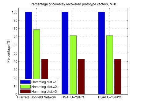
Refer to caption
Figure 6: The figure shows percentage of correctly recovered desired patterns for all possible initial conditions in example 3 for the proposed DSALU-”SIR”1 and DSALU-”SIR”2 as compared to traditional discrete Hopfield network with 8 neurons.

As seen from Figure 6, the performances of the DSALU-”SIR”1 and 2 are the same as that of the discrete-time Hopfield Network for 1-Hamming distance case (%100\%100 for both networks) and are comparable for 2 and 3-Hamming distance cases respectively.

Example 4:

The desired prototype vectors as well as the obtained weight matrices are given in in Appendix II (eq.(178)).

For matrix r𝐈𝑟𝐈r{\bf I}, ρ𝜌\rho is chosen as -2. The other network paramaters are chosen as in example 3.

The Figure 7 shows the percentages of correctly recovered desired patterns for all possible initial conditions 𝐱(k=0)(1,+1)16𝐱𝑘0superscript1116\mathbf{x}(k=0)\in(-1,+1)^{16}, in the proposed DSALU”SIR”1 and 2 as compared to the traditional Hopfield network.
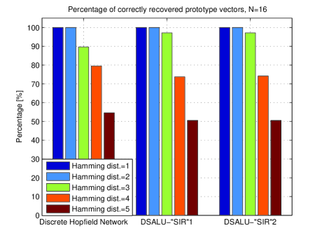
Refer to caption
Figure 7: The figure shows percentage of correctly recovered desired patterns for all possible initial conditions in example 4 for the proposed DSALU-”SIR”1 and DSALU-”SIR”2 as compared to the traditional discrete Hopfield network with 16 neurons.

The total number of different possible combinations for the initial conditions for this example is 64, 480 and 2240 and 7280 for 1, 2, 3 and 4-Hamming distance cases respectively.

As seen from Figure 7 the performance of the proposed networks DSALU-”SIR”1 and 2 are the same as that of Hopfield Network for 1 and 2-Hamming distance cases (%100\%100 for both networks), and are comparable for 3,4 and 5-Hamming distance cases respectively.

V Conclusions

In this paper, we present and analyse two Hopfield-like nonlinear networks, in continuous-time and discrete-time respectively. The proposed network is based on an autonomous linear system with a symmetric weight matrix, which is designed to be unstable, and a nonlinear function stabilizing the whole network thanks to a manipulated state variable. This variable is observed to be equal to the traditional Signal-to-Interference Ratio (SIR) definition in telecommunications engineering.

The underlying linear system of the proposed continuous-time network is 𝐱˙=𝐁𝐱˙𝐱𝐁𝐱\dot{{\mathbf{x}}}={\mathbf{B}}{\mathbf{x}} where B is a real symmetric matrix whose diagonal elements are fixed to a constant. The nonlinear function, on the other hand, is based on the defined system variables called “SIR”s. We also show that the “SIR”s of all the states converge to a constant value, called “system-specific Ultimate SIR”; which is equal to rλmax𝑟subscript𝜆𝑚𝑎𝑥\frac{r}{\lambda_{max}} where r𝑟r is the diagonal element of matrix 𝐁𝐁{\bf B} and λmaxsubscript𝜆𝑚𝑎𝑥\lambda_{max} is the maximum (positive) eigenvalue of diagonally-zero matrix (𝐁r𝐈)𝐁𝑟𝐈({\bf B}-r{\bf I}), where 𝐈𝐈{\bf I} denotes the identity matrix. The same result is obtained in its discrete-time version as well.

Computer simulations for binary associative memory design problem show the effectiveness of the proposed network as compared to the traditional Hopfield Networks.

Acknowledgments

This work was supported in part by Academy of Finland and Research Foundation (Tukisäätiö) of Helsinki University of Technology, Finland.

The author would also like to thank the anonymous four reviewers for their valuable comments which helped in improving the structure and the content of the paper.

References

  • [1] J.J. Hopfield and D.W Tank, Neural computation of decisions in optimization problems Biological Cybernetics, vol. :141-146, 1985.
  • [2] S. Matsuda, “Optimal” Hopfield network for combinatorial optimization with linear cost function, IEEE Trans. Neural Networks, vol. 9: 1319-1330, Nov. 1998.
  • [3] K. Smith, M. Palaniswami, and M. Krishnamoorthy, Neural techniques for combinatorial optimization with applications, IEEE Trans. Neural Networks, vol. 9: 1301-1318, Nov. 1998.
  • [4] K.C. Tan, T. Huajin and S.S. Ge, On parameter settings of Hopfield networks applied to traveling salesman problems, Circuits and Systems I, vol. 52, nr. 5: 994-1002, May 2005.
  • [5] T. Huajin, K.C. Tan and Y. Zhang, A columnar competitive model for solving combinatorial optimization problems, IEEE Trans. Neural Networks, vol. 15, nr. 6: 1568 - 1574, Nov. 2004.
  • [6] J.K. Paik and A.K. Katsaggelos, Image restoration using a modified Hopfield network, IEEE Trans. Image Processing, vol. 1, nr. 1:49-63, Jan. 1992.
  • [7] J.A. Farrel and A.N. Michel, A synthesis procedure for Hofield’s continuous-time associative memory, IEEE Trans. Circuits Systems, vol. 37: 877 - 884, 1990.
  • [8] G.G. Lendaris, K. Mathia and R. Saeks, Linear Hopfield networks and constrained optimization IEEE Trans. Systems, Man, and Cybernetics, Part B, vol. 29, nr. 1: 114 - 118 Feb. 1999.
  • [9] S. Haykin, Neural Networks, Macmillan, 1999.
  • [10] J.M. Zurada, Introduction to Artificial Neural Systems, West Publishing Company, 1992.
  • [11] M.K. Muezzinoglu, M.K. and C. Guzelis, A Boolean Hebb rule for binary associative memory design, IEEE Trans. Neural Networks, vol. 15, nr. 1:195 - 202, Jan. 2004.
  • [12] M.K. Muezzinoglu, C. Guzelis and J.M. Zurada, An energy function-based design method for discrete hopfield associative memory with attractive fixed points, IEEE Trans. Neural Networks, vol. 16, nr. 2:370-378, March 2005 .
  • [13] T.S. Rappaport, Wireless Communications: Principles and Practice, Prentice-Hall, New York, 1996.
  • [14] Z. Uykan, “From Sigmoid Power Control Algorithm to Hopfield-like Neural Networks: “SIR” (“Signal”-to-“Interference”-Ratio)- Balancing Sigmoid-Based Networks”, to be resubmitted to IEEE Trans. Neural Networks in September 2009.
  • [15] D. O. Hebb, The Organization of Behaviour , John Wiley and Sons, New York, 1949.
  • [16] O. Bretscher, Linear Algebra with Applications, Prentice Hall, 2005.
  • [17] D. Luenberger, Introduction to Dynamic Systems: Theory, Models and Applications, John Wiley and Sons, Inc. New York, 1979.
  • [18] G. M. Pan and W. Zhou Central limit theorem for signal-to-interference ratio of reduced rank linear receiver, Annals of Applied Probability, DOI: 10.1214/07-AAP477, vol. 18, no. 3: 1232-1270, 2008. (arXiv:0806.2768v1 [math.PR]).

Appendix I

In Example 2, the matrix which has the desired prototype vectors as its raws is

𝐃=[1111111111111111111111111111111111111111111111111111111111111111]𝐃delimited-[]1111111111111111111111111111111111111111111111111111111111111111{\mathbf{D}}=\left[\begin{array}[]{c c c c c c c c c c c c c c c c}1&1&1&1&1&1&1&1&-1&-1&-1&-1&-1&-1&-1&-1\\ 1&1&1&1&-1&-1&-1&-1&1&1&1&1&-1&-1&-1&-1\\ 1&1&-1&-1&1&1&-1&-1&1&1&-1&-1&1&1&-1&-1\\ 1&-1&1&-1&1&-1&1&-1&1&-1&1&-1&1&-1&1&-1\end{array}\right] (158)

In Example 2, the weight matrices r𝐈𝑟𝐈r{\bf I} and 𝐖𝐖{\bf W}, which are obtained by the outer products based design as explained in Section III-C, are as follows:

r𝐈𝑟𝐈\displaystyle r{\mathbf{I}} =\displaystyle= 2𝐈2𝐈\displaystyle 2{\mathbf{I}} (159)
𝐖𝐖\displaystyle{\mathbf{W}} =\displaystyle= [0220200220020224200202200220204220020220022024020220200220024220200202200224200202202002204202200220200224020220200202204220200220020224022020020220204220020220022024022002022020024220022020020224200220020220204202200220200224020220022020024220200220020220]delimited-[]0220200220020224200202200220204220020220022024020220200220024220200202200224200202202002204202200220200224020220200202204220200220020224022020020220204220020220022024022002022020024220022020020224200220020220204202200220200224020220022020024220200220020220\displaystyle\left[\begin{array}[]{c c c c c c c c c c c c c c c c}0&2&2&0&2&0&0&-2&2&0&0&-2&0&-2&-2&-4\\ 2&0&0&2&0&2&-2&0&0&2&-2&0&-2&0&-4&-2\\ 2&0&0&2&0&-2&2&0&0&-2&2&0&-2&-4&0&-2\\ 0&2&2&0&-2&0&0&2&-2&0&0&2&-4&-2&-2&0\\ 2&0&0&-2&0&2&2&0&0&-2&-2&-4&2&0&0&-2\\ 0&2&-2&0&2&0&0&2&-2&0&-4&-2&0&2&-2&0\\ 0&-2&2&0&2&0&0&2&-2&-4&0&-2&0&-2&2&0\\ -2&0&0&2&0&2&2&0&-4&-2&-2&0&-2&0&0&2\\ 2&0&0&-2&0&-2&-2&-4&0&2&2&0&2&0&0&-2\\ 0&2&-2&0&-2&0&-4&-2&2&0&0&2&0&2&-2&0\\ 0&-2&2&0&-2&-4&0&-2&2&0&0&2&0&-2&2&0\\ -2&0&0&2&-4&-2&-2&0&0&2&2&0&-2&0&0&2\\ 0&-2&-2&-4&2&0&0&-2&2&0&0&-2&0&2&2&0\\ -2&0&-4&-2&0&2&-2&0&0&2&-2&0&2&0&0&2\\ -2&-4&0&-2&0&-2&2&0&0&-2&2&0&2&0&0&2\\ -4&-2&-2&0&-2&0&0&2&-2&0&0&2&0&2&2&0\end{array}\right] (176)

Appendix II

In Example 4, the matrix which has the desired prototype vectors as its raws is

𝐃=[111111111111111111111111111111111111111111111111]𝐃delimited-[]111111111111111111111111111111111111111111111111{\mathbf{D}}=\left[\begin{array}[]{c c c c c c c c c c c c c c c c}1&1&1&1&1&1&1&1&-1&-1&-1&-1&-1&-1&-1&-1\\ 1&1&1&1&-1&-1&-1&-1&1&1&1&1&-1&-1&-1&-1\\ 1&1&-1&-1&1&1&-1&-1&1&1&-1&-1&1&1&-1&-1\end{array}\right] (178)

In Example 4, the weight matrices r𝐈𝑟𝐈r{\bf I} and 𝐖𝐖{\bf W} obtained are as follows:

r𝐈𝑟𝐈\displaystyle r{\mathbf{I}} =\displaystyle= 3𝐈,3𝐈\displaystyle 3{\mathbf{I}},
𝐖𝐖\displaystyle{\mathbf{W}} =\displaystyle= [0311111111111133301111111111113311031111111133111130111111113311111103111133111111113011113311111111110333111111111111303311111111111133031111111111113330111111111133111103111111113311113011111133111111110311113311111111301133111111111111033311111111111130],delimited-[]0311111111111133301111111111113311031111111133111130111111113311111103111133111111113011113311111111110333111111111111303311111111111133031111111111113330111111111133111103111111113311113011111133111111110311113311111111301133111111111111033311111111111130\displaystyle\left[\begin{array}[]{c c c c c c c c c c c c c c c c}0&3&1&1&1&1&-1&-1&1&1&-1&-1&-1&-1&-3&-3\\ 3&0&1&1&1&1&-1&-1&1&1&-1&-1&-1&-1&-3&-3\\ 1&1&0&3&-1&-1&1&1&-1&-1&1&1&-3&-3&-1&-1\\ 1&1&3&0&-1&-1&1&1&-1&-1&1&1&-3&-3&-1&-1\\ 1&1&-1&-1&0&3&1&1&-1&-1&-3&-3&1&1&-1&-1\\ 1&1&-1&-1&3&0&1&1&-1&-1&-3&-3&1&1&-1&-1\\ -1&-1&1&1&1&1&0&3&-3&-3&-1&-1&-1&-1&1&1\\ -1&-1&1&1&1&1&3&0&-3&-3&-1&-1&-1&-1&1&1\\ 1&1&-1&-1&-1&-1&-3&-3&0&3&1&1&1&1&-1&-1\\ 1&1&-1&-1&-1&-1&-3&-3&3&0&1&1&1&1&-1&-1\\ -1&-1&1&1&-3&-3&-1&-1&1&1&0&3&-1&-1&1&1\\ -1&-1&1&1&-3&-3&-1&-1&1&1&3&0&-1&-1&1&1\\ -1&-1&-3&-3&1&1&-1&-1&1&1&-1&-1&0&3&1&1\\ -1&-1&-3&-3&1&1&-1&-1&1&1&-1&-1&3&0&1&1\\ -3&-3&-1&-1&-1&-1&1&1&-1&-1&1&1&1&1&0&3\\ -3&-3&-1&-1&-1&-1&1&1&-1&-1&1&1&1&1&3&0\end{array}\right], (195)