Target Detection via Network Filtering

Abstract

A method of ‘network filtering’ has been proposed recently to detect the effects of certain external perturbations on the interacting members in a network. However, with large networks, the goal of detection seems a priori difficult to achieve, especially since the number of observations available often is much smaller than the number of variables describing the effects of the underlying network. Under the assumption that the network possesses a certain sparsity property, we provide a formal characterization of the accuracy with which the external effects can be detected, using a network filtering system that combines Lasso regression in a sparse simultaneous equation model with simple residual analysis. We explore the implications of the technical conditions underlying our characterization, in the context of various network topologies, and we illustrate our method using simulated data.

Keywords: Sparse network, Lasso regression, network topology, target detection.

I Introduction

A canonical problem in statistical signal and image processing is the detection of localized targets against complex backgrounds, which often is likened to the proverbial task of ‘finding a needle in a haystack’. In this paper, we consider the task of detecting such targets when the ‘background’ is neither a one-dimensional signal nor a two-dimensional image, but rather consists of the ‘typical’ behavior of interacting units in a network system. More specifically, we assume network-indexed data, where measurements are made on each of the units in the system and the interaction among these units manifests itself through the correlations among these measurements. Then, given the possible presence of an external effect applied to a unit(s) of this system, we take as our goal the task of identifying the location and magnitude of this effect. It is expected that evidence of this effect be diffused throughout the system, to an extent determined by the underlying network of interactions among system units, like the blurring of a point source in an image. As a result, an appropriate filtering of the observed measurements is necessary. These ideas are illustrated schematically in Figure 1.

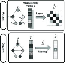
Figure 1: Schematic illustration of the network filtering process proposed in this paper, shown in two stages. In the first stage, the aim is to recover information on the correlation (i.e., $\hat{B}$) among the five network units, given training data $Y$. In the second stage, that information is used to filter new data $\tilde{Y}$, produced in the presence of an effect external to the system (i.e., $\phi$), so as to detect the target of that effect.

While networks have been an important topic of study for some time, in recent years there has been an enormous surge in interest in the topic, across various diverse areas of science. Examples include computer traffic networks (e.g., [10]), biological networks (e.g., [1]), social networks (e.g., [25]), and sensor networks (e.g., [23]). Our network filtering problem was formulated by, and is largely motivated by the work of, Cosgrove et al.[8], who used it to tackle the problem of predicting genetic targets of biochemical compounds proposed as candidates for drug development. However, the problem is clearly general and it is easy to conceive of applications in other domains.

The authors in [8] model the acquisition of network data, including the potential presence of targets, using a system of sparse simultaneous equation models (SSEMs), and propose to search for targets using a simple two-step procedure. In the first step, sparse statistical inference techniques are used to remove the ‘background’ of network effects, while in the second step, outlier detection methods are applied to the resulting network-filtered data. Empirical work presented in [8], using both simulated data and real data from micro-array studies, demonstrates that such network filtering can be highly effective. However, there is no accompanying theoretical work in [8].

In this paper, we present a formal characterization of the performance of network filtering, exploring under what conditions the methodology can be expected to work well. A collection of theoretical results are provided, which in turn are supported by an extensive numerical study. Particular attention is paid to the question of how network structure influences our ability to detect external effects. The technical aspects of our work draw on a combination of tools from the literatures on sparse regression and compressed sensing, complex networks, and spectral graph theory.

The remainder of the paper is organized as follows. The basic SSEM model and two-step network filtering methodology are presented formally in Section II. In Section III we characterize the accuracy with which the network effects can be learned from training data, while in Section IV, we use these results to quantify the extent to which external effects will be evident in test data after filtering out the learned network effects. Numerical results, based on simulations under various choices of network structure, are presented in Section V. Finally, we conclude with some additional discussion in Section VI. Proofs of all formal results are gathered in the appendices.

II Network Filtering: Model and Methodology

Consider a system of $p$ units (e.g., genes, people, sensors, etc.). We will assume that we can take measurements at each unit, and that these measurements are likely correlated with measurements at some (small) fraction of other units, such as might occur through ‘interaction’ among the units. For example, in [8], where the units are genes, the measurements are gene expression levels from microarray experiments. Genes regulating other genes can be expected to have expression profiles correlated across experiments. Alternatively, we could envision measuring environmental variables (e.g., temperature) at nodes in a sensor network. Sensors located sufficiently close to each other, with respect to the dynamics of the environmental process of interest, can be expected to yield correlated readings.

We will also assume that there are two possible types of measurements: a training set, obtained under ‘standard’ conditions, and a test set measured under the influence of additional ‘external’ effects. The training set will be used to learn patterns of interaction among the units (i.e., our ‘network’), and with that knowledge, we will seek to identify in the test data those units targeted by the external effects.

We model these two types of measurements using systems of simultaneous equation models (SEMs). Formally, suppose that for each of the $p$ units, we have in the training set $n$ replicated measurements, which are assumed to be realizations of the elements of a random vector $Y=(Y_{1},\ldots,Y_{p})^{\prime}$. Let $Y_{i}$ be the i-th element of $Y$, and let $Y_{[-i]}$ denote all elements of $Y$ except $Y_{i}$. We specify a conditional linear relationship among these elements, in the form

$$Y_{i}\,\big{|}\,Y_{[-i]}=y_{[-i]}\quad\,{\buildrel d\over{=}}\,\quad\sum_{j\neq i}^{p}\beta_{ij}y_{j}+e_{i}\enskip,$$ (1)

where $\beta_{ij}$ represents the strength of association of the measurement for the i-th unit with that of the j-th unit, and $e_{i}$ are error terms, assumed to be independently distributed as $N(0,\sigma^{2})$. That is, we specify a so-called ‘conditional Gaussian model’ for the $Y_{i}$, which in turn yields a joint distribution for $Y$ in the form

$${Y}\,\sim\,N\left(\,0\,,\,(I-B)^{-1}\sigma^{2}\,\right),$$ (2)

with $B$ being a matrix whose $(i,j)$ entry $B_{ij}$ is $\beta_{ij}$, for $i\neq j$, and zero otherwise. See [9, Ch 6.3.2]. The matrix $I-B$ is assumed to be positive definite. In addition, we will assume $B$ (and hence $I-B$) to be sparse, in the sense of having a substantial proportion of its entries equal to zero. A more precise characterization of this assumption is given below, in the statement of Theorem 1.

We can associate a network with this model using the framework of graphical models (e.g., [19]). Let each unit in our system correspond to a vertex in a vertex set $V=\{1,\ldots,p\}$, and define an edge set $E$ such that $\{i,j\}\in E$ if and only if $B_{ij}\neq 0$. Then the model in (2), paired with the graph $G=(V,E)$, is a Gaussian graphical model, with concentration (or ‘precision’) matrix $\Omega=(I-B)\sigma^{-2}$ and concentration graph $G$. Since we assume $B$ to be sparse, the graph $G$ likewise will be sparse. Gaussian graphical models are a common choice for modeling multivariate data with potentially complicated correlation (and hence dependency) structure. This structure is encoded in the graph $G$, and questions regarding the nature of this structure often can be rephrased in terms of questions involving the topology of $G$. In recent years, there has been increased interest in modeling and inference for large, sparse Gaussian graphical models of the type we consider here (e.g., [11, 21]).

For the test set, our observations are assumed to be realizations of another random vector, say $\tilde{Y}=(\tilde{Y}_{1},\ldots,\tilde{Y}_{p})^{\prime}$, the elements of which differ from those of $Y$ only through the possible presence of an additive perturbation. That is, we model each $\tilde{Y}_{i}$, conditional on the others, as

$$\tilde{Y}_{i}\,\big{|}\,\tilde{Y}_{[-i]}=\tilde{y}_{[-i]}\quad\,{\buildrel d\over{=}}\,\quad\sum_{j\neq i}^{p}\beta_{ij}\tilde{y}_{j}+\phi_{i}+\tilde{e}_{i}\enskip,$$ (3)

where $\phi_{i}$ denotes the effect of the external perturbation for the i-th unit, and the error terms $\tilde{e}_{i}$ are again independently distributed as $N(0,\sigma^{2})$. Similar to (2), we have in this scenario

$${\tilde{Y}}\,\sim\,N\left(\,(I-B)^{-1}\phi\,,\,(I-B)^{-1}\sigma^{2}\,\right)\enskip,$$ (4)

where $\phi=(\phi_{1},\ldots,\phi_{p})^{\prime}$.

The external effects $\phi$ are assumed unknown to us but sparse. That is, we expect only a relatively small proportion of units to be perturbed. Our objective is to estimate the external effects $\phi$ and to detect which units $i$ were perturbed i.e., to detect those units $i$ for which $\phi_{i}$ stands out from zero above noise. But we do not observe the external effects $\phi$ directly. Rather, these effects are ‘blurred’ by the network of interactions captured in $B$, as indicted by the expression for the mean vector in (4). If $B$ were known, however, it would be natural to filter the data $\tilde{Y}$, producing

$$\hat{\phi}^{ideal}=(I-B)\tilde{Y}\enskip.$$ (5)

The random vector $\hat{\phi}^{ideal}$ has a multivariate Gaussian distribution, with expectation $\phi$ and covariance $(I-B)\sigma^{2}$. Hence, element-wise, each $\hat{\phi}^{ideal}_{i}$ is distributed as $N(\phi_{i},\sigma^{2})$, and therefore the detection of perturbed units $i$ reduces to detection of a sparse signal against a uniform additive Gaussian noise, which is a well-studied problem. Note that under this model, we expect the noise in $\hat{\phi}^{ideal}$ to be correlated. However, given the assumptions of sparsity on $B$, these correlations will be relatively localized.

Of course, $B$ typically is not known in practice, and so $\hat{\phi}^{ideal}$ in (5) is an unobtainable ideal. Studying the same problem, Cosgrove et al. [8] proposed a two-stage procedure in which (i) $p$ simultaneous sparse regressions are performed to infer $B$, row-by-row, yielding an estimate $\hat{B}$, and (ii) the ideal residuals in (5) are predicted by the values

$$\hat{\phi}=(I-\hat{B})\tilde{Y}\enskip,$$ (6)

after which detection is carried out. They dubbed this overall process ‘network filtering’. A schematic illustration of network filtering is shown in Figure 1.

Our central concern in this paper is with characterizing the conditions under which network filtering can be expected to work well. Motivated by the original context of Cosgrove et al., involving a network of gene interactions and measurements based on micro-array technology, we assume here that (i) $p\gg n$, (ii) the matrix $B$ is sparse, and (iii) the vector $\phi$ is sparse. In carrying out our study, we adopt a strategy for estimating $B$ based on Lasso regression [24], a now-canonical example of sparse regression. Specifically, motivated by (1), we estimate each row $B_{i\bullet}$ as

$$\hat{B}_{i\bullet}\stackrel{{\scriptstyle\triangle}}{{=}}\arg\min_{\beta\in\mathbb{R}^{p}:\beta_{ii}=0}\|y_{i}-\sum_{j\neq i}^{p}\beta_{ij}y_{j}\|^{2}_{2}+\mu\|\beta\|_{1}\ ,$$ (7)

where $\mu>0$ is a regularization parameter. Following this estimation stage, we carry out detection using simple rank-based procedures.

We present our results in two stages, first describing conditions under which $\hat{B}$ estimates $B$ accurately, given the system of sparse simultaneous equation models (SSEMs) defined by (1), and then discussing the nature of the resulting vector $\hat{\phi}$. In both stages, we explore the implications of the topological structure of $G$ on our results.

III Accuracy in estimation of $B$

At first glance, accurate estimation of $B$ seems impossible, since even if the error terms $e_{i}$ are small, this noise typically will be inflated by naive inversion of our systems of equations (i.e., because $p\gg n$). However, recent work on analogous problems in other models has shown that under certain conditions, and using tools of sparse inference, it is indeed possible to obtain good estimates. Results of this nature have appeared under the names ‘compressed sensing’, ‘compressive sampling’, and similar. See the recent review [6], and the references therein. The following result is similar in spirit to these others, for the particular sparse simultaneous equation models we study here.

Theorem 1

Assume the training model defined in (1) and (2), and set $\Sigma=(I-B)^{-1}\sigma^{2}$. Let $S$ be the largest number of non-zero entries in any row of $B$, and suppose that $\Sigma,S,p,$ and $n$ satisfy the conditions

$$\frac{\lambda_{max}(\Sigma)}{\lambda_{min}(\Sigma)} \leq \left(\frac{1+\sqrt{S/n}}{1-\sqrt{S/n}}\right)^{2}$$ (8)

and

$$\rho(r) < 1\enskip.$$ (9)

Here $\lambda_{max}$ and $\lambda_{min}$ refer to maximum and minimum eigenvalues and $\rho(r)=(1+f(4r))^{2}+2(1+f(5r))^{2}-3$, where $r=S/(p-1)$ and $f$ is a function to be defined latter. Finally, assume that $\mu^{2}\leq(C_{0}\sigma^{2}\zeta_{n}^{-})/S$, for a constant $C_{0}=C_{0}(n,p,r)$ and $\zeta_{n}^{-}=n\left(1-4(\log_{2}n/n)^{1/2}\right)$. Let $p=n^{\nu}$, for $\nu>1$. Then it follows that, with overwhelming probability, for every row $B_{i\bullet}$ of $B$ the estimator $\hat{B}_{i\bullet}$ in (7) satisfies the relation

$$\|\hat{B}_{i\bullet}-B_{i\bullet}\|^{2}_{2}\leq C\sigma^{2}\zeta_{n}^{+}\enskip,$$ (10)

where $\zeta_{n}^{+}=n\left(1+4(\log_{2}n/n)^{1/2}\right)$ and $C>0$ is a constant.

Remark 1: The accuracy of $\hat{B}_{i\bullet}$ is seen in (10) to depend primarily on the product $n\sigma^{2}$ and on $C$. The constant $C$ can be bounded by an expression of the form $(1-\rho(r))^{-2}$ times a constant depending only on the structure of $\Sigma$. The magnitude of $C$ therefore is controlled essentially by the extent to which $\rho(r)$ is less than $1$, which in turn is a rough reflection of the sparsity of the network. Hence, in order to have good accuracy, $\sigma^{2}$ must be small compared to $n^{-1}$. In particular, if $\sigma^{2}=O(n^{-\omega})$, for $\omega>1$, then the error in (10) behaves roughly like $O\left(n^{-(\omega-1)}\right)$.

Remark 2: Clearly it cannot be expected that we estimate $B$ with high accuracy in all situations. The expressions in (8) and (9) dictate sufficient conditions under which, with overwhelming probability (meaning with probability decaying exponentially in $p$), we can expect to do well. Due to the intimate connection between the covariance $\Sigma$ and the concentration graph $G$, these conditions effectively place restrictions on the structure of the network we seek to filter, with (8) controlling the relative magnitude of the eigenvalues of the matrix $I-B$, and (9), its sparseness. Note that since $S$ is simply the maximum degree of $G$, condition (9) relates the maximum extent of the degree distribution of $G$ to the sample size $n$. We explore the nature of these conditions in more detail immediately below.

Remark 3. In general, of course, choice of the Lasso regularization parameter $\mu>0$ in (7) matters. The statement of Theorem 1 includes constraints on the range of acceptable values for this parameter. In particular, it suggests that $\mu$ should vary like $\sigma^{2}n/S$, which for $\sigma^{2}=O(n^{-\omega})$ means we want $\mu=O(S^{-1}n^{-(\omega-1)})$. The theorem does not, however, provide explicit guidance on how to set this parameter in practice. For the empirical work shown later in this paper, we have used cross-validation, which we find yields results like those predicted by the theorem over a broad range of scenarios.

Remark 4. There are results in the literature that address other problems sharing certain aspects of our network filtering problem, but none that address all together. For example, the bound in (10) is like that in work by Candès and Tao and colleagues (e.g., [4, 5]), although for a single regression, rather than a system of simultaneous regressions. In addition, those authors use constrained minimization for parameter estimation, rather than Lasso-based optimization. As Zhu [26] has recently pointed out, there are small but important differences in these closely related problems. Our proof makes use of Zhu’s results. Similarly, Greenshtein and Ritov [15] present results for models that – in principle at least – include the individual univariate regressions in (1), although again their results do not encompass a system of such regressions. Furthermore, their results are in terms of mean-squared prediction error, rather than in terms of the regression coefficients themselves. Finally, Meinshausen and Bühlmann [21] have studied the use of Lasso in the context of Gaussian graphical models, but for the purpose of recovering the topology of $G$ i.e., for variable selection, rather than parameter estimation. The proof of Theorem 1 may be found in Appendix A.

In the remainder of this section, we examine conditions (8) and (9) in greater depth. These conditions derive from our use of certain concentration inequalities, which – although central to the proof of our result – can be expected to be somewhat conservative. Our numerical results, shown later, confirm this expectation. Nonetheless, these conditions are useful in that they help provide insight into the way that the network topology structure, on the one hand, and the sample size $n$, on the other, can be expected to interact in determining the performance of our network filtering methodology.

III-A The eigenvalue constraint

Recall that the covariance matrix $\Sigma$ is proportional to $(I-B)^{-1}$. In order to better understand the condition on the covariance matrix in (8), consider the special case of

$$\Sigma^{-1}=(I-B)=I+qD^{-1/2}AD^{-1/2}\enskip,$$ (11)

where $A$ is the adjacency matrix for a graph $G$, $D=\hbox{diag}[(d_{i})]_{i\in V}$ is a diagonal matrix, $d_{i}$ is the degree (i.e., the number of neighbors) of vertex $i$, and $q>0$ is a constant. Here the covariance $\Sigma$ is defined entirely in terms of the topology of the concentration graph $G$. While later, in Sections 3 and 4, we use simulation to explore more complicated covariance structures, where the $B_{ij}$ are assigned randomly according to certain distributions, the simplified form in (11) is useful in allowing us to produce analytical results. In particular, conditions on $\Sigma$ reduce to conditions on our network topology. For example, the following theorem describes a sufficient condition under which (8) holds for this model.

Theorem 2

Suppose that the covariance matrix $\Sigma$ from Theorem 1 is defined through (11), with $0<q<1$. Denote

$$\eta_{1}=\frac{\sum_{i=1}^{p}\frac{\sum_{j\sim i}1/d_{j}}{d_{i}}}{p}\ \hbox{and}\ \eta_{2}=\left(\frac{1+\sqrt{d_{\max}/n}}{1-\sqrt{d_{\max}/n}}\,\Big{/}\,\sqrt{2}\right)^{4/p},$$ (12)

where $i\sim j$ indicates that the vertices $i$ and $j$ are neighbors in $G$ and $d_{max}=\max_{1\leq i\leq p}d_{i}$ is the maximum vertex degree. Then condition (8) on the eigenvalues of $\Sigma$ is satisfied if

$$\frac{1}{(1+q)^{2}}+(\frac{q}{1+q})^{2}\,\eta_{1}\leq\eta_{2}\enskip.$$ (13)

Proof of this result may be found in Appendix B. The restriction on $q$ ensures that the matrix $\Sigma^{-1}$ is diagonally dominant, which is needed for our proof, although it likely could be weakened. Note that the condition in (13) involves the graph $G$ only through the degree sequence $\{d_{1},\ldots,d_{p}\}$. More precisely, this condition relates the average harmonic mean of neighbor degrees (i.e., $\eta_{1}$) and the maximum degree to the sample size $n$ and the constant $q$. Accordingly, given a network, it is straightforward to explore the implications of this condition numerically. For example, we can explore the range of values $q$ for which the condition holds, given $n$.

Figure 2: Plots of ER, BA, and geometric random graphs of size $p=100$ and average degree $\bar{d}=4$.

Figure 2 shows examples of three network topologies. The first is an Erdös-Rényi (ER) random graph[13], a classical form of random graph in which vertex pairs $i,j$ are assigned edges according to independently and identically distributed Bernoulli random variables (i.e., coin flips). The degree distribution of an ER network is concentrated around its mean and has tails that decay exponentially fast. The second is a random graph generated according to the Barabási and Albert model [2], which was originally motivated by observed structure in the World Wide Web. The defining characteristic of the BA model is that the derived network has a degree distribution of a power-law form, with tails decreasing like $d^{-3}$ for large $d$. Therefore, the BA networks tend to contain many vertices with only a few neighbors, and a few vertices with many neighbors. Lastly, we also use a geometric random graph model, such as might be appropriate for modeling spatial networks. Following[21], vertices in the graph are uniformly distributed throughout the unit square $[0,1]^{2}$, and each vertex pair $i,j$ has an edge with probability $\phi\left(w_{ij}p^{1/2}\right)$, where $\phi(\cdot)$ is the standard normal density function and $w_{ij}$ is the Euclidean distance in $[0,1]^{2}$ between $i$ and $j$. In all three cases, the random graph was of size $p=100$ and had average degree $\bar{d}=4$.

In Figure 3 we show the eigenvalue ratio in (8), under the simplified covariance structure in (11), for these ER, BA,and geometric random graphs, as a function of $q$.

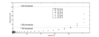
Figure 3: Plots of eigenvalue ratio for ER, BA, and geometry graph under different values of $q$.

The horizontal lines represent the theoretical eigenvalue ratio bound given by Theorem 1. The open symbols (including the ‘plus’ symbol) indicate graphs that satisfy the condition in Theorem 2, while the filled symbols indicate graphs that do not satisfy the condition. We can see from the plot that the condition in Theorem 2 clearly is conservative, since as a function of $q$ it ceases to hold long before the inequality in (8) is violated.

III-B The sparsity constraint

The second condition in Theorem 1, given in (9), can be read as a condition on the sparsity $r=S/(p-1)$ of the precision matrix $\Omega\propto I-B$, and therefore a condition on the sparsity of our network graph $G$. The analytical form of the function $\rho(\cdot)$ is

$$\rho(r)=(1+f(4r))^{2}+2(1+f(5r))^{2}-3\enskip,$$ (14)

where $f(r)=\sqrt{p/n}\left(\sqrt{r}+\sqrt{2H(r)}\right),$ and $H(r)=-r\log(r)-(1-r)\log(1-r)$ is the entropy function. While it is not feasible to produce a closed-form solution in $r$ to the inequality (9), it is straightforward to explore the space of solutions numerically.

Note that $\rho(r)$ actually is a function of the three parameters $S$, $p$, and $n$ through the two ratios $S/(p-1)$ and $n/p$. In practice we expect both ratios to be in the interval $(0,1)$. Shown in Figure 4 is $\rho(\cdot)$, as a function of $r$, for a handful of representative choices of $n/p$. We see from the plot that the theory suggests, through condition (9), that the sparsity $r$ should be bounded by roughly $1\times 10^{-4}$. Our numerical results, however, shown later, indicate that the theory is quite conservative, in that, for example, for our simulations we successfully used networks with sparsity on the order of $r=0.04$. Analogous observations have been made in [4]. Also shown in Figure 4 is a 3D plot of $\rho(\cdot)$, as a function of both $r$ and $n/p$. In this plot, the dark area corresponding to the innermost contour line satisfies the condition that $\rho(r)<1$. Again, the value of the information shown here is primarily as an indication of the existence of feasible combinations of $S$, $p$, and $n$ allowing for the accurate estimation of the rows of $B$.

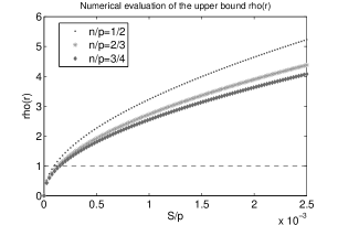
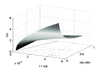
Figure 4: 2D plot and 3D plot showing the behavior of $\rho_{n/p}(r)$ for three values of the ratio $n/p$.

IV Accuracy of the network filtering

With the accuracy of $\hat{B}$ quantified, we turn our attention to the effectiveness of our filtering of the network effects. Specifically, in the following theorem we characterize the behavior of $\hat{\phi}$, defined in (6), as a predictor of $\hat{\phi}^{ideal}$, defined in (5).

Theorem 3

Suppose $\tilde{Y}$ is a $p\times 1$ vector of test data, obtained according to the model defined in (3) and (4). Let $\hat{\phi}=(I-\hat{B})\tilde{Y}$ be defined as in (6) and let $\Delta=B-\hat{B}$. Then conditional on $\hat{B}$, $\hat{\phi}$ has a multivariate normal distribution, with expectation and variance

$$E\left[\hat{\phi}\,\big{|}\,\hat{B}\right]=\phi+\Delta(I-B)^{-1}\phi$$ (15)

$$\operatorname{Var}\left[\hat{\phi}\,\big{|}\,\hat{B}\right]=(I-B)\sigma^{2}+\left[\,\Delta(I-B)^{-1}\Delta^{T}+2\Delta\,\right]\,\sigma^{2}\enskip.$$ (16)

Furthermore, under the conditions of Theorem 1, element-wise we have

$$\left|\,E\left[(\hat{\phi}_{i}-\phi_{i})\,\big{|}\,\hat{B}\right]\,\right|\leq||\phi||_{2}\,\left[\,(C\sigma^{2}\zeta_{n}^{+})^{1/2}\,\lambda_{max}\left((I-B)^{-1}\right)\,\right]$$ (17)

and

$$\operatorname{Var}\left[\hat{\phi}_{i}\,\big{|}\,\hat{B}\right]\leq\sigma^{2}\left[\,1+C\sigma^{2}\zeta_{n}^{+}\lambda_{max}\left((I-B)^{-1}\right)\,\right]\enskip,$$ (18)

with overwhelming probability, where $C>0$ and $\zeta_{n}^{+}$ are as in Theorem 1.

Proof of this theorem may be found in Appendix C. Recall that $\hat{\phi}^{ideal}$ in (5) is distributed as a multivariate normal random vector, with expectation $\phi$ and variance $(I-B)\sigma^{2}$. Equations (15) and (16) show that our predictor $\hat{\phi}$ mimics $\hat{\phi}^{ideal}$ well to the extent that our error in estimating $B$ – that is, those terms involving $\Delta$ – are small. Theorem 1 quantifies the magnitude of the rows $\Delta_{i\bullet}=B_{i\bullet}-\hat{B}_{i\bullet}$ of $\Delta$, from which we obtain the term $C\sigma^{2}\zeta_{n}^{+}$ in our bounds on the element-wise predictive bias in (17) and variance in (18).

Remark 4: In the case that there are no external effects exerted upon our system i.e., $\phi=0$, the elements $\hat{\phi}^{ideal}_{i}$ of the ideal estimate $\hat{\phi}^{ideal}$ are just identically distributed $N(0,\sigma^{2})$ noise. This case corresponds to the intuitive null distribution we might use to formulate our detection problem as a statistical hypothesis testing problem. The implication of the theorem is that, in using $\hat{\phi}$ rather than $\hat{\phi}^{ideal}$, following substitution of $\hat{B}$ for $B$, the price we pay is that the elements $\hat{\phi}_{i}$ are instead distributed as $N(0,\tilde{\sigma}^{2}_{i})$, where the $\tilde{\sigma}^{2}_{i}$ differ from $\sigma^{2}$ by no more than $C\sigma^{2}\zeta_{n}^{+}\lambda_{max}\left((I-B)^{-1}\right)$. Treating $\lambda_{max}\left((I-B)^{-1}\right)$ as a constant for the moment, this term is dominated by $C\sigma^{2}\zeta_{n}^{+}$ i.e., our error in estimating the rows of $B$. Hence, for example, if $\sigma^{2}=O(n^{-\omega})$ with $\omega>1$, as in Remark 1, then the variances $\tilde{\sigma}^{2}_{i}$ will also be $O(n^{-\omega})$.

Remark 5: Suppose instead that $\phi=(0,\ldots,0,\phi^{*},0,\ldots,0)^{\prime}$, for some $\phi^{*}>0$. This case corresponds to the simplest alternative hypothesis we might use, involving a non-trivial perturbation, and is a reasonable proxy for the type of ‘genetic perturbations’ (e.g., from gene knock-out experiments) considered in Cosgrove et al.[8]. Now the bias is potentially non-zero, even for units $i$ with $\phi_{i}=0$. But, again treating $\lambda_{max}\left((I-B)^{-1}\right)$ as a constant, and assuming $\sigma^{2}=O(n^{-\omega})$, this bias will be only negligibly worse than the $O(n^{-(\omega-1)/2})$ magnitude of the ideal standard deviation $\sigma$. And the variance will again be $O(n^{-\omega})$. Therefore, we should be able to detect single-unit perturbations well for $\phi^{*}$ sufficiently above the noise. Our simulation results in the next section confirm this expectation.

Now consider the term $\lambda_{max}\left((I-B)^{-1}\right)$, which reflects the effect of the topology of $G$ on our ability to do detection with network filtering. This term will not necessarily be a constant in $n$, due to the role of $n$ in the bounds (8) and (9) of Theorem 1, constraining the behavior of $\Sigma=(I-B)^{-1}\sigma^{2}$. The following lemma lends some insight into the behavior of this term in the case where the precision matrix $\Omega=\Sigma^{-1}$ again has the simple form specified in (11). The proof may be found in Appendix C.

Lemma 1

Suppose that $\Sigma^{-1}=I+qD^{-1/2}\,A\,D^{-1/2}$, as in (11). Then

$$\lambda_{max}\left((I-B)^{-1}\right)\leq\frac{\sqrt{d_{max}}}{q+\sqrt{d_{max}}}\,\left(\frac{1+\sqrt{d_{max}/n}}{1-\sqrt{d_{max}/n}}\right)^{2}\enskip.$$ (19)

Remark 6: Because we assume that the network $G$ will be sparse, and that $d_{max}<n$, the above result indicates that the term $\lambda_{max}\left((I-B)^{-1}\right)$ can be treated under our simplified covariance as a constant essentially with respect to $\sigma^{2}\zeta_{n}^{+}$ in expressions like (17) and (18).

V Simulation Results

V-A Background

In this section, we use simulated network data to further study the performance of our proposed network filtering method. The data are drawn from the models for training and test data defined in Section II, with randomly generated covariance matrices $\Sigma$. We define these covariances through their corresponding precision matrices $\Omega=\Sigma^{-1}$, which are obtained in turn by (i) generating a random network topology $G=(V,E)$, and then (ii) assigning random weights to entries in $\Omega$ corresponding to pairs $i,j$ with edges $\{i,j\}\in E$. These collections of weights are then rescaled in a final step to coerce $\Omega$ into the form $I-B$ and, if necessary, to enforce positive definiteness. For the topology $G$, we use the three classes of random network topologies $G=(V,E)$ described above in Section III.A i.e., the ER, BA, and geometric networks. For each choice of network, we use $p=100$ nodes, each of which has an average degree of $\bar{d}=4$. The adjacency matrices $A$ of the ER and BA model are generated randomly using the algorithms listed in [3], while that of the geometric network is generated according to the method described in [21].

In implementing our network filtering method, the Lars [12] implementation of the Lasso optimization in (7) was used, on training data sets of various sample sizes for each network. The Lasso regularization parameter $\mu$ was chosen by cross-validation. To generate testing data, we used single-unit perturbations of the form $\phi=(0,\ldots,0,\phi^{*},0,\ldots,0)^{\prime}$, where $\phi^{*}>0$ is in the $i$-th position, for each $i=1,\ldots,100$. Since $\sigma^{2}$ in our simulation is effectively set to $1$, $\phi^{*}$ can be interpreted as the signal-to-noise ratio (SNR) of the underlying perturbation. In our simulations, we let $\phi^{*}$ range over integers from $1$ to $20$. Our final objective of detection is to find the position of the unit at which the external perturbation occurred. In our proposed network filtering method, we declare the perturbed unit to be that corresponding to the entry of $\hat{\phi}$ with largest magnitude i.e., $\hat{i}=\arg\max_{1\leq i\leq p}|\hat{\phi}_{i}|$.

In each experiment described below, our method is compared with two other methods. The first, called ‘True’, is that in which the ideal $\hat{\phi}^{ideal}$ is used instead of $\hat{\phi}$, which presumes knowledge of the true $B$. The second, called ‘Direct’, is that in which the actual testing data $\tilde{Y}$ i.e., the data without network filtering, are used instead of $\hat{\phi}$. In both cases, we declare the perturbed unit to be that corresponding to the entry of largest magnitude. The ‘True’ method gives us a benchmark for the detection error under the ideal situation that we already have all of the network information, while the ‘Direct’ method is a natural approach in the face of having no information on the network. By comparing our method with the two, we may gauge how much is gained by using the network filtering method. In all cases, performance error is quantified as the fraction of times a perturbed unit is not correctly identified i.e., the proportion of mis-detections. Results reported below for all three methods are based in each case upon $30$ replicates of the testing data. Our plots show average proportions of mis-detections and one standard deviation.

V-B Results

First we present the results from an experiment where $\Sigma$ is defined according to the simple formulation given in (11), the definition that underlays the results in Theorem 2 and Lemma 1. That is, we define $\Sigma$ in terms of just the (random) adjacency structure of our three underlying networks, scaled by an appropriate choice of $q$ to ensure positive definiteness. We may think of this case, from the perspective of the simulation design described above, as one with a particular non-random choice of weights for edges in the network $G$ i.e., where $B=-qD^{-1/2}AD^{-1/2}$.

Figure 5 shows the average proportions of mis-detections, as a function the SNR, for these three models. Note that since the underlying graphs are random, there is some variability in such detection results from simulation to simulation. However, these plots and the others below like them are representative in our experience. From the plots in the figure, we can see that in all cases the network filtering offers a significant improvement over the ‘Direct’ method, and in fact comes reasonably close to matching the performance of the ‘True’ method, with mis-detections at a rate of roughly 5-25% for high SNR. Performance differs somewhat with respect to networks of different topology. The network filtering method shows the most gain over the ‘Direct’ method with the BA network. This phenomenon is consistent with our intuition: the distribution of edges in the BA network is the least uniform one, and certain choices of perturbed unit (i.e., perturbed units $i$ with large degree $d_{i}$) will enable the effects of perturbation to spread comparatively widely. Hence obtaining and correcting for the internal interactions among units in the network is particularly helpful in this case.

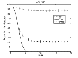
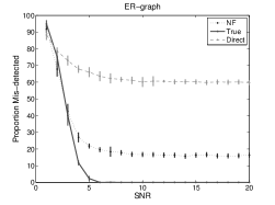
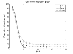
Figure 5: Plots of the proportion of mis-detections versus signal-to-noise ratio, for the BA, ER and geometric random networks, based on the simplified covariance model in (11), using $q=1.25$, $p=100$ and $n=50$. Error bars indicate one standard error over $30$ test datasets.

Now consider the assignment of random weights to edges in $G$, which allows us to generate a richer variety of models. For this purpose, we choose the family of beta distributions $Beta(a,b)$ from which to draw weights $B_{ij}$ independently for each edge $\{i,j\}\in E$. Three different classes of distributions were used i.e., $Beta(1,1)$, $Beta(1/2,1/2)$, and $Beta(2,2)$, which gives flat (uniform), U-shape, and peaked shape forms. Shown in Figure 6 are the results of our network filtering method, the ‘True’ method, and the ‘Direct’ method, for each of these three choices of weight distributions, for each of the three network topologies. The same (random) network topology is used in each plot for each type of network.

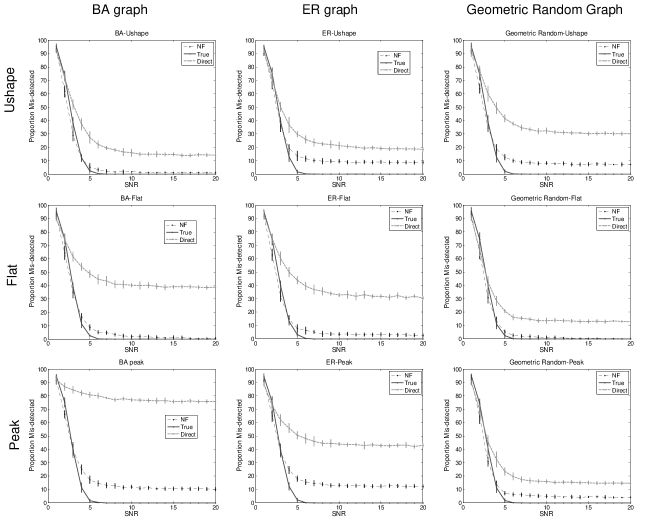
Figure 6: Plots of proportions of mis-detections versus signal-to-noise ratio. Columns: BA (left), ER (middle), and geometric (right) random networks. Rows: U-shaped (top), flat (middle), and peaked (bottom) choice of weight distributions, generated according to $Beta(1/2,1/2)$, $Beta(1,1)$ and $Beta(2,2)$ distributions, respectively.

Broadly speaking, these plots show that the performance of network filtering in the context of randomly generated edge weights $B_{ij}$, as compared to that of the ‘True’ and ‘Direct’ methods, is essentially consistent with the case of fixed edge-weights underlying the plots in Figure 5. However, there are some interesting nuances. For example, in the case of ‘Flat’ weights, network filtering in fact is able to match the performance of ‘True’ for all three classes of graphs. On the other hand, in the ER random network topology this matching occurs only when the edge-weight distribution is flat (i.e., $Beta(1,1)$), and in the BA random network topology, when the distribution is either $U$-shaped (i.e., $Beta(1/2,1/2)$) or flat (i.e., $Beta(1,1)$). Nevertheless, the qualitatively similar performance across choice of edge-weight distribution suggests that most important element here is the network structure, indicating connection between pairs of units, with the strength of connection being secondary.

Finally, we consider the effect of sample size $n$ and, therefore implicitly, the extent to which the condition in (8) on the structure of the covariance matrix $\Sigma$ may be relaxed. For the same networks used in the simulations described above, with $p=100$ units, we varied the sample size $n$ to range over $20,50,100$, and $150$. Weights of the network edges are set according to a $Beta(2,2)$ distribution, which is the ‘peak’ case. Training and testing data were generated as before. The results of using network filtering in these different settings are shown in Figure 7. Again, our network filtering method is seen to work similar to above. Even for a sample size as small as $n=20$, our method still does better than the ‘Direct’ method in all three models, particularly under the BA and ER models.

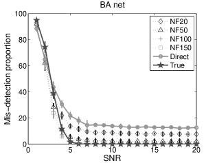
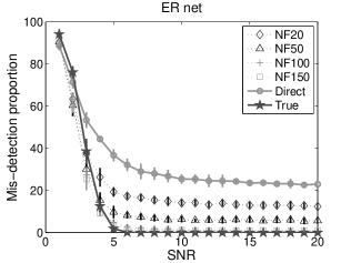
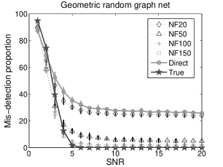
Figure 7: Plots of proportion of mis-detections versus signal-to-noise ratio for the BA (left), ER (middle), and geometric (right) random network models, for sample sizes $n=20,50,100$, and $150$.

On a final note, we point out that in all of the experiments the richness of network models studied is much broader than suggested by our theory. As was mentioned earlier, the concentration inequalities we use can be expected to be conservative in nature, and therefore some of the bounds are more restrictive than practice seems to indicate is necessary. For example, in our simulations involving the geometric random graph in Figure 2, with a sample size of $n=50$ and $S=9$, the theoretical bound (8) for the eigenvalue ratio is $6.12$, while the actual value achieved by this ratio is $219$ in this instance. Also, the maximum degrees of the graphs in most of the simulations are larger than the average degree 4, and hence the sparseness rate $S/p>4/100$, which is already larger than those theoretical sparse rates suggested by Figure 1. Yet still we observed the network filtering method to perform quite well. It is an interesting open question to see if the theory can be extended to produce bounds like (8) that more accurately reflect practice, to serve as a better practical guides for users.

VI Discussion

The concept of network filtering considered in this paper was first proposed by Cosgrove et al. [8], as a methodology for filtering out the effects of ‘typical’ gene regulatory patterns in DNA microarray expression data, so as to enhance the potential signal from genetic targets of putative drug compounds. Here we have formalized the methodology of Cosgrove et al. and established basic conditions under which it may be expected to perform well. Furthermore, we have explored the implications of these conditions on the topology of the network underlying the data (i.e., a Gaussian concentration graph). Proof of our results rely on principles and techniques central to the literature on compressed sensing and, therefore, like other results in that literature, make performance statements that hold with over-whelming probability. Numerical simulation results strongly suggest a high degree of robustness of the methodology to departure from certain of the basic conditions stated in our theorems regarding network topology. Our current work is now focused on the development of adaptive learning strategies that intentionally utilize perturbations (i.e., in the form of the vectors $\phi$) to more efficiently explore network effects (i.e., the matrix $B$).

Appendix A Proof of the First Zonklar Equation

Appendix B Proof of Theorem 1

Theorem 1 jointly characterizes the accuracy of $p$ simultaneous regressions, each based on the model in (1) i.e., for $i=1,\ldots,p$,

$$y_{i}=\sum_{j\neq i}^{p}\beta_{ij}y_{j}+e_{i}\enskip.$$ (20)

For convenience, we re-express the above model for a single regression in the generic form

$$R=X\beta+e\enskip.$$ (21)

Here $X$ is a $n\times(p-1)$ design matrix with rows sampled i.i.d. from a multivariate normal distribution $N(0,\mathbb{C})$, with $(p-1)\times(p-1)$ covariance matrix $\mathbb{C}$; $e$ is an $n\times 1$ error vector, independent of $X$, with i.i.d. $N(0,\sigma^{2})$ elements; and $R$ is the $n\times 1$ response vector.

We will make use of a result of Zhu [26], which requires the notion of restricted isometry constants. Following Zhu, we define the $S$-restricted isometry constant $\delta_{S}$ of the matrix $X$ as the smallest quantity such that

$$(1-\delta_{S})\|c\|_{2}\leq\|X_{T}c\|_{2}\leq(1+\delta_{S})\|c\|_{2}$$ (22)

for all index subsets $T\subset\{1,\ldots,p\}$ with $|T|\leq S$. Zhu’s result is then as follows.

Lemma 2 (Zhu)

If (i) the number of non-zero entries of $\beta$ is no more than $S$, (ii) the isometry constants $\delta_{4S}$ and $\delta_{5S}$ obey the inequality $\delta_{4S}+2\delta_{5S}<1$, and (iii) the Lasso regularization parameter $\mu$ obeys the constraint $\mu^{2}\leq C_{0}\zeta/S$, for $\zeta=||e||^{2}_{2}$, then

$$||\beta-\hat{\beta}||^{2}_{2}\leq\tilde{C}\zeta\enskip,$$ (23)

where

$$\hat{\beta}=\arg\min_{\beta}\|X\beta-R\|^{2}_{2}+\mu\|\beta\|_{1}\enskip.$$ (24)

Zhu’s first condition is assumed in our statement of Theorem 1. Therefore, to prove Theorem 1 we need to show, under the other conditions stated in our theorem, that Zhu’s second and third conditions above hold simultaneously for each of our $p$ regressions, with overwhelming probability. In addition, we need to show that the right-hand side of (23) is bounded above by the right-hand side of (10).

B-A Verification of Lemma 24, Condition (ii)

The essence of what is needed for the restricted isometry constants is contained in the following lemma.

Lemma 3

Suppose $\mathbb{C}_{T}$ is a sub-matrix of the covariance matrix $\mathbb{C}$ with columns variables corresponding to these in $\mathbb{C}$ of the indices in set $T$, where $|T|=S$. Denote the largest and smallest eigenvalues of any such matrix $\mathbb{C}_{T}$ as $\lambda_{max}(\mathbb{C}_{T})$ and $\lambda_{min}(\mathbb{C}_{T})$ respectively. Suppose too that

$$\frac{\lambda_{max}(\mathbb{C}_{T})}{\lambda_{min}(\mathbb{C}_{T})}\leq\left(\frac{1+\sqrt{S/n}}{1-\sqrt{S/n}}\right)^{2}\quad\hbox{and}\quad\rho(r)<1\enskip,$$ (25)

where $\rho(r)$ is defined as in (14). Then the condition $\delta_{4S}(X)+2\delta_{5S}(X)<1$ holds with overwhelming probability.

The covariance matrix $\mathbb{C}$ corresponding to any single regression is a sub-matrix of $\Sigma$ in Theorem 1, and hence so is any sub-sub-matrix $\mathbb{C}_{T}$. By the interlacing property of eigenvalues (e.g., Golub and van Loan [14, Thm 8.1.7]), which relates the eigenvalues of a symmetric matrix to those of its principle sub-matrices, as long as $\Sigma$ satisfies the eigenvalue constraint (8), the matrices $\mathbb{C}_{T}$ will as well. So it is sufficient to prove Lemma 3.

Proof of Lemma 3: Let $X_{T}$ denote the $n\times S$ sub-matrix of $X$ corresponding to the subset of indices $T$. Since the rows of $X$ are independent samples from $N(0,\mathbb{C})$, the rows of $X_{T}$ are independent samples from $N(0,\mathbb{C}_{T})$. Let $\sigma_{i}$ be the i-th largest singular value of $\mathbb{C}_{T}^{1/2}$ and $\hat{\sigma}_{i}$ be the i-th largest singular value of $n^{-1/2}X_{T}$. The eigenvalue condition in the lemma reduces to $(\sigma_{1}/\sigma_{S})\leq\left[1+(S/n)^{1/2}\right]/\left[1-(S/n)^{1/2}\right]$. Without loss of generality, therefore, assume that $\sigma_{1}\leq 1+(S/n)^{1/2}$ while $\sigma_{S}\geq 1-(S/n)^{1/2}$.

Note we can express $X_{T}$ as $X_{T}=Z\mathbb{C}_{T}^{1/2}$, where $Z\sim N(0,I)$. Then $X_{T}^{\prime}X_{T}=[\mathbb{C}^{1/2}_{T}]^{\prime}Z^{\prime}Z\mathbb{C}^{1/2}_{T}$ and hence the eigenvalues of $X_{T}^{\prime}X_{T}$ are the same as those of $Z^{\prime}Z\mathbb{C}_{T}$. Thus we have

$$\lambda_{\max}\left(\frac{X_{T}^{\prime}X_{T}}{n}\right) \leq \lambda_{\max}\left(\frac{Z^{\prime}Z}{n}\right)\cdot\sigma_{1}^{2}$$ (26)

$$\lambda_{\min}\left(\frac{X_{T}^{\prime}X_{T}}{n}\right) \geq \lambda_{\min}\left(\frac{Z^{\prime}Z}{n}\right)\cdot\sigma_{S}^{2}.$$ (27)

Let $\hat{\sigma}_{i}^{*}$ denote the i-th largest singular value of $n^{-1/2}Z$. Therefore we have

$$\hat{\sigma}_{1} \leq \hat{\sigma}_{1}^{*}\cdot\sigma_{1}$$ (28)

$$\hat{\sigma}_{S} \geq \hat{\sigma}_{S}^{*}\cdot\sigma_{s}$$ (29)

Denote by $\hat{\sigma}_{min}(\cdot),\hat{\sigma}_{max}(\cdot)$ the smallest and largest singular values of their argument. Notice that for any index set $T^{*}\subset T$, we have

$$\hat{\sigma}_{min}\left(\frac{X_{T}}{\sqrt{n}}\right)\leq\hat{\sigma}_{min}\left(\frac{X_{T^{*}}}{\sqrt{n}}\right)\leq\hat{\sigma}_{max}\left(\frac{X_{T^{*}}}{\sqrt{n}}\right)\leq\hat{\sigma}_{max}\left(\frac{X_{T}}{\sqrt{n}}\right).$$

Thus we need only to consider the situation where $|T|=S$ and choose $\delta$ as the smallest constant that satisfies (22) for any sub-matrix $X_{T}$ of size $n\times S$. Therefore, we set $1-\delta\leq\tilde{\sigma}_{S}\leq\tilde{\sigma}_{1}\leq 1+\delta,$ where $\tilde{\sigma}_{1}=\sup_{|T|=S}\hat{\sigma}_{1}$ and $\tilde{\sigma}_{S}=\inf_{|T|=S}\hat{\sigma}_{S}$. It then follows that $\delta\leq\max(1-\tilde{\sigma}_{S},\tilde{\sigma}_{1}-1).$

Now, by the large deviation results in [20, 4], for a standard Gaussian random matrix $Z\sim N(0,I)$, there are two relevant concentration inequalities:

$$P\left(\hat{\sigma}_{1}^{*}>1+\sqrt{S/n}+\eta+t\right) \leq e^{-nt^{2}/2}$$ (30)

$$P\left(\hat{\sigma}_{S}^{*}<1-\sqrt{S/n}-\eta-t\right) \leq e^{-nt^{2}/2},$$ (31)

where $\eta$ is an $o(1)$ term.

We can then use the above tools and concentration inequalities to see how $\delta$ behaves under the conditions described in Lemma 3. Notice that, for $\varepsilon>0$, we have

$$P\left(1+\delta>(1+(1+\varepsilon)f(r))^{2}\right)$$ (32)

$$\leq P\left(\max(2-\tilde{\sigma}_{S}\ ,\tilde{\sigma}_{1}\right)\geq(1+(1+\varepsilon)f(r))^{2})$$ (33)

$$= P\left(\{2-\tilde{\sigma}_{S}\geq(1+(1+\varepsilon)f(r))^{2}\}\cup\right.$$ (35)

$$\left\{\tilde{\sigma}_{1}\geq(1+(1+\varepsilon)f(r))^{2}\}\right)$$

$$\leq P\left(\tilde{\sigma}_{S}\leq 2-(1+(1+\varepsilon)f(r))^{2})\right)$$ (37)

$$+P\left(\tilde{\sigma}_{1}\geq(1+(1+\varepsilon)f(r))^{2}\right)$$

Denoting $\gamma=S/n$, we have by (29) that $\hat{\sigma}_{S}\geq(1-\sqrt{\gamma})\hat{\sigma}_{S}^{*}$. Therefore, for the term with $\tilde{\sigma}_{S}$ in (37), we have by Bonferroni’s inequality that

$$P\left(\tilde{\sigma}_{S}\leq 2-(1+(1+\varepsilon)f(r))^{2})\right)$$

$$\leq \sum_{\{|T|=S\}}P\left(\hat{\sigma}_{S}(X_{T})\leq 2-(1+(1+\varepsilon)f(r))^{2})\right)$$

$$\leq |\{|T|=S\}|P\left((1-\sqrt{\gamma})\cdot\hat{\sigma}_{S}^{*}\leq 2-(1+(1+\varepsilon)f(r))^{2})\right)$$

$$\leq C(p,S)\cdot$$

$$P\left((1-\sqrt{\gamma})\cdot\hat{\sigma}_{S}^{*}\leq 1-2(1+\varepsilon)f(r)-((1+\varepsilon)f(r))^{2}\right)$$

$$\leq C(p,S)P\left(\hat{\sigma}_{S}^{*}\leq 1-(1+\varepsilon)f(r)\right)\enskip.$$

As in [4], we fix $\eta+t=(1+\varepsilon)\sqrt{p/n}\sqrt{2H(r)}$, from which it follows that $(1+\varepsilon)f(r)\simeq\sqrt{\frac{S}{n}}+\eta+t$ and $C(p,s)e^{-nt^{2}/2}\leq e^{-pH(r)\varepsilon/2}$. Hence the above inequality is equivalent to

$$P\left(\tilde{\sigma}_{S}\leq 2-(1+(1+\varepsilon)f(r))^{2})\right)$$

$$\leq C(p,S)P\left(\hat{\sigma}_{S}^{*}\leq(1-\sqrt{S/n}-\eta-t)\right)$$

$$\leq C(p,S)e^{-nt^{2}/2}$$

$$\leq e^{-pH(r)\varepsilon/2}$$

For the term with $\tilde{\sigma}_{1}$ in (37), the analogous inequality

$$P(\tilde{\sigma}_{1}\geq(1+(1+\varepsilon)f(r))^{2})\leq e^{-pH(r)\varepsilon/2}$$

may be verified using a similar argument. Combining these two probability inequalities for $\tilde{\sigma}_{1}$ and $\tilde{\sigma}_{S}$, we have that $P\left(1+\delta>(1+(1+\varepsilon)f(r))^{2}\right)\leq 2\cdot e^{-pH(r)\varepsilon/2}.$ Ignoring the negligible $\varepsilon$ terms, it follows that when $p,n$ is large enough $\delta<(1+f(r))^{2}-1$ holds with overwhelming probability. Defining $\rho(r)=(1+f(4r))^{2}+2(1+f(5r))^{2}-3$, we have that $\delta_{4S}+2\delta_{5S}<\rho(r)$. Imposing the condition $\rho(r)<1$, we obtain that $\delta_{4S}+2\delta_{5S}<1$, and therefore Lemma 3 is proved.

B-B Verification of Lemma 24, Condition (iii) and the right-hand side of (10)

Let $R^{(i)}=X^{(i)}\beta^{(i)}+e^{(i)}$ denote the regression equation (21) for the $i$-th of the $p$ simultaneous regressions in (20). Condition (iii) of Lemma 24 requires that the regularization parameter $\mu$ be such that $\mu^{2}\leq C_{0}\zeta^{(i)}/S$, where $\zeta^{(i)}=||e^{(i)}||^{2}_{2}$. If so, and assuming of course that conditions (i) and (ii) are satisfied as well, then the inequality in (23) says that $||\hat{\beta}^{(i)}-\beta^{(i)}||^{2}_{2}\leq C^{(i)}\zeta^{(i)}$. We show that the condition on $\mu$ in the statement of Theorem 1 i.e., that $\mu^{2}\leq(C_{0}\sigma^{2}\zeta_{n}^{-})/S$, guarantees that Condition (iii) holds for every $i=1,\ldots,p$ with overwhelming probability. In addition, we show that $C^{(i)}\zeta^{(i)}\leq C\sigma^{2}\zeta_{n}^{+}$ with overwhelming probability, where $\zeta_{n}^{+}=n\left(1+4(\log_{2}n/n)^{1/2}\right)$, and $C$ is bounded by $(1-\rho(r))^{-2}$ times a constant, as claimed in Remark 1.

Notice that if we have $e\sim N(0,\sigma^{2}I_{n\times n})$, then $||e||^{2}_{2}$ is distributed as chi-square on $n$ degrees of freedom. By [18, Sec 4.1, Lemma 4], for $t^{\prime}>0$,

$$P\left\{\|e\|^{2}_{2}-n\sigma^{2}\leq-4\sigma^{2}\sqrt{nt^{\prime}}\right\}\leq\exp(-t^{\prime})$$

and

$$P\left\{\|e\|^{2}_{2}-n\sigma^{2}\geq 4\sigma^{2}\sqrt{nt^{\prime}}\right\}\leq\exp(-t^{\prime})\enskip.$$

Therefore,

$$P\left\{\min_{i}\frac{\|e^{(i)}\|^{2}_{2}}{n\sigma^{2}}\leq(1-4\sqrt{t^{\prime}/n})\right\}$$

$$\leq\sum_{i=1}^{p}P\left\{\frac{\|e^{(i)}\|^{2}_{2}}{n\sigma^{2}}\leq(1-4\sqrt{t^{\prime}/n})\right\}$$

$$=pP\left\{\frac{\|e\|^{2}_{2}}{n\sigma^{2}}\leq(1-4\sqrt{t^{\prime}/n})\right\}\leq p\exp(-t^{\prime})\enskip,$$

and similarly,

$$P\left\{\max_{i}\frac{\|e^{(i)}\|^{2}_{2}}{n\sigma^{2}}\geq(1+4\sqrt{t^{\prime}/n})\right\}\leq p\exp(-t^{\prime})\enskip.$$

We choose $t^{\prime}$ so that $\mu^{2}\leq C_{0}||e^{(i)}||^{2}_{2}/S$ uniformly in $i$ with probability at least $1-2e^{-pH(r)\epsilon/2}$, so as to match the rate in Section A above. Specifically, we set $t^{\prime}=\left[pH(r)\varepsilon\right]/2+\log\left(p/2\right)$. Hence, for sufficiently small $\varepsilon$ we have $t^{\prime}\approx\log(p/2)$. Therefore, as long as $\mu^{2}\leq\left(C_{0}\sigma^{2}n/S\right)\left[1-4(t^{\prime}/n)^{1/2}\right]$, then with probability exceeding $1-2e^{-pH(r)\varepsilon/2}$, the inequality $\mu^{2}\leq C_{0}||e^{(i)}||^{2}_{2}/S$ holds uniformly in $i$. Suppose $p=n^{\nu}$, with $\nu>1$. Under this condition, $t^{\prime}/n\approx\left(\log_{2}n^{\nu}\right)/n=\nu\left(\log_{2}n\right)/n$ and our requirement thus reduces to $\mu^{2}\leq\left(C_{0}\sigma^{2}n/S\right)\left[1-4\left((\log_{2}n)/n\right)^{1/2}\right]$. Similarly, with $t^{\prime}\approx\log\left(p/2\right)$, we also have with probability exceeding $1-2e^{-pH(r)\varepsilon/2}$ that $\|e^{(i)}\|_{2}^{2}\leq\sigma^{2}n\left[1+4\left((\log_{2}n)/n\right)^{1/2}\right]$.

Let $\zeta_{n}^{-}$ and $\zeta_{n}^{+}$ be defined as in the statement of Theorem 1. Then by requiring that $\mu^{2}\leq(C_{0}\sigma^{2}\zeta_{n}^{-})/S$, from the above results it follows that Condition (iii) of Lemma 2 holds for all $i=1,\ldots,p$, with high probability. Furthermore, with high probability, $||e^{(i)}||^{2}_{2}\leq\sigma^{2}\zeta_{n}^{+}$, for $i=1,\ldots,p$. Therefore, by the bound (23) in Lemma 2, we have established the bound (10) in Theorem 1, except for the constant $C$.

Specifically, it remains for us to establish that $C^{(i)}\leq C$ for all $i$. Denote the value $C^{(i)}$ for an arbitrary regression by $\tilde{C}$. Note that the $\tilde{C}$ here in our paper corresponds to the square of what is called ‘$C$’ in Zhu [26]. Hence by equation (17) in [26], $\tilde{C}^{1/2}$ is smaller than the larger root of a quadratic equation of the form

$$a^{2}z^{2}-(2ac+b)z+(c^{2}-\tau)=0\enskip,$$

where $z$ is the argument and $a,b,c$ and $\tau$ are positive parameters. For our purposes, it is enough to remark that $a>(1-\delta_{4S}-2\delta_{5S})/3$, $b$ is bounded by a constant proportional to $C_{0}^{1/2}$, $c$ relates to $a$ through the expression $a=c\left[2\mu S^{1/2}/\zeta^{1/2}\right]-1-\delta_{4S}$, and $\tau$ is a constant greater than four,

As the larger root of the above quadratic equation,

$$\tilde{C}^{1/2}\leq\frac{2ac+b+\sqrt{(2ac+b)^{2}-4a^{2}(c^{2}-\tau)}}{2a^{2}}\enskip.$$

Note that $(2ac+b)^{2}-4a^{2}(c^{2}-\tau)=4abc+b^{2}+4a^{2}\tau$, which is bounded by $\max((2a\tau^{1/2}+b)^{2},(2ac+b)^{2})$, because $a,b,c$ and $\tau$ are all positive. Hence we have

$$\tilde{C}^{1/2} \leq \max\left(\frac{2ac+b+2a\tau^{1/2}+b}{2a^{2}},\frac{2ac+b+2ac+b}{2a^{2}}\right)$$ (38)

$$< \max\left(\frac{\tau^{1/2}+c}{a}+\frac{b}{a^{2}},\frac{2c}{a}+\frac{b}{a^{2}}\right)$$

$$< 2\,\frac{\max(c,\tau^{1/2})}{a}+\frac{b}{a^{2}}\enskip.$$

It remains for us to bound the right-hand side of (38). Recall that, by construction, $\delta_{4S}+2\delta_{5S}\leq\rho(r)$, and that $\rho(r)$ is assumed strictly less than $1$. Thus, because $b$ is bounded by a term proportional to $C_{0}^{1/2}$, the second term in the right-hand side of (38) is bounded by a term proportional to $(1-\rho(r))^{2}$. Furthermore, if $\tau^{1/2}\geq c$, then the first term is bounded by a term proportional to $(1-\rho(r))$. Lastly, therefore, suppose that $c>\tau^{1/2}$ and consider the term

$$\frac{c}{a}=\frac{1}{2\mu S^{1/2}/\zeta^{1/2}}\,\frac{a+1+\delta_{4S}}{a}\enskip.$$ (39)

The term involving $a$ in the right-hand side of (39) is easily bounded, per our reasoning above, while – taking, for example, $\mu^{2}=C_{0}\zeta/S$ in the condition of Lemma 24, the other term is equal to $(4C_{0})^{-1/2}$.

Hence, returning to the context of our original problem, for each $i=1,\ldots,p$, the constant $C^{(i)}$ is bounded by some constant times $(1-\rho(r))^{-2}$. Letting $C$ be the largest of these bounds, our proof of Theorem 1 is complete.

Appendix C Proof for Theorem 2

To show that condition (8) of Theorem 1 holds in the context of Theorem 2, we first bound the eigenvalue ratio of the covariance matrix $\Sigma$. For $q\in(0,1)$, the matrix $\Sigma^{-1}$ is diagonally dominant, and hence, by the Levy-Desplanques Theorem, non-singular. Furthermore, since $\Sigma^{-1}$ is real and symmetric, it is a normal matrix. Therefore,

$$\frac{\lambda_{\max}(\Sigma)}{\lambda_{\min}(\Sigma)}=\frac{1/\lambda_{\min}(\Sigma^{-1})}{1/\lambda_{\max}(\Sigma^{-1})}=\frac{\lambda_{\max}(\Sigma^{-1})}{\lambda_{\min}(\Sigma^{-1})}=\kappa_{2}(\Sigma^{-1}),$$

where $\kappa_{2}(\Sigma^{-1})$ is condition number of the precision matrix $\Sigma^{-1}$. As a result, by an inequality of Guggenheimer, Edelman, and Johnson [16, Pg. 4] for condition numbers, we can bound our eigenvalue ratio as

$$\frac{\lambda_{\max}(\Sigma)}{\lambda_{\min}(\Sigma)}\leq\frac{2}{|\det(\Sigma^{-1})|}\left(\frac{\|\Sigma^{-1}\|_{F}^{2}}{p}\right)^{p/2}\enskip.$$ (40)

Since $\Sigma^{-1}=I+qD^{-1/2}AD^{-1/2}$, direct calculation shows that

$$\|\Sigma^{-1}\|_{F}^{2} = p+q^{2}\|D^{-1/2}AD^{-1/2}\|_{F}^{2}=p+q^{2}\sum_{i\sim j}(\frac{1}{\sqrt{d_{i}d_{j}}})^{2}$$

$$= p+q^{2}\sum_{i=1}^{p}\frac{1}{d_{i}}\sum_{j\sim i}\frac{1}{d_{j}}\enskip,$$

where $d_{i}$ is the i-th element of the diagonal matrix $D$. As for the quantity $|\det(\Sigma^{-1})|$, we note that

$$|\det(\Sigma^{-1})| = |q\det(D^{-1/2})\det(1/qD+A)\det(D^{-1/2})|$$

$$= q^{p}\prod_{i=1}^{p}d_{i}^{-1}|\det(1/qD+A)|\enskip.$$

Denoting $M=(1/q)D+A$, and applying a result of Ostrowski for determinants of diagonally dominant matrices (e.g., [22]), we find that

$$|\det(M)|\geq\prod_{i=1}^{p}(|M_{ii}|+\sum_{j\neq i}|M_{ij}|) = \prod_{i=1}^{p}(\frac{1}{q}d_{i}+d_{i})$$

$$= \left(\frac{1+q}{q}\right)^{p}\prod_{i=1}^{p}d_{i}\enskip.$$

Hence, we have $\det(\Sigma^{-1})\geq(1+q)^{p}$.

Combining the relevant expressions above, we have that

$$\frac{\lambda_{\max}(\Sigma)}{\lambda_{\min}(\Sigma)}\leq\frac{2}{(1+q)^{p}}\left(1+\frac{q^{2}\sum_{i=1}^{p}\frac{\sum_{j\sim i}1/d_{j}}{d_{i}}}{p}\right)^{p/2}$$ (41)

$$= 2\left[\frac{1}{(1+q)^{2}}+(\frac{q}{1+q})^{2}\operatorname{Ave}_{i}\left(HM_{j\sim i}(\frac{1}{d_{j}})\right)\right]^{p/2}\enskip.$$ (42)

Denoting $\eta_{1}$ and $\eta_{2}$ as in (12), bounding the right-hand side of (42) by $\left[1+(d_{max}/n)^{1/2}\right]/\left[1-(d_{max}/n)^{1/2}\right]$, to enforce the bound (8), and some trivial manipulation of the resulting inequality, yields the condition in (13), as desired.

Appendix D Proof for Theorem 3

Note that the difference of the predictor $\hat{\phi}$ and the true external effect $\phi$ is given as $\hat{\phi}-\phi=\tilde{Y}-\hat{B}\tilde{Y}-\phi=(I-\hat{B})\tilde{Y}-\phi$. So the bias term is just

$$E[(\hat{\phi}-\phi)|\hat{B}]=(I-\hat{B})(I-B)^{-1}\phi-\phi$$

$$=[(I-\hat{B})-(I-B)](I-B)^{-1}\phi=\Delta(I-B)^{-1}\phi\enskip,$$

where $\Delta=B-\hat{B}$, and hence for the i-th component of the bias term, we have

$$\left|E\left[(\hat{\phi}_{i}-\phi_{i})\,\big{|}\,\hat{B}\right]\right| = \left|\Delta_{i\bullet}(I-B)^{-1}\phi\right|$$

$$\leq \|\Delta_{i\bullet}\|_{2}\quad\|(I-B)^{-1}\|_{2}\quad\|\phi\|_{2}$$

$$\leq \left[(C\sigma^{2}\zeta_{n}^{+})^{1/2}\,\,\lambda^{1/2}_{max}\left((I-B)^{-1}\right)\right]\,\,\|\phi\|_{2}\enskip.$$

Here the first term in brackets follows from Theorem 1, while the second follows from the definition of the $\ell_{2}$ matrix norm.

For the variance of the predictor $\hat{\phi}$, we have

$$\operatorname{Var}\left[\hat{\phi}\mid\hat{B}\right]=(I-\hat{B})(I-B)^{-1}(I-\hat{B})^{T}\sigma^{2}$$

$$= (I-B+B-\hat{B})(I-B)^{-1}(I-B+B-\hat{B})^{T}\sigma^{2}$$

$$= (I-B)\sigma^{2}+\left[\Delta(I-B)^{-1}\Delta^{T}+2\Delta\right]\sigma^{2}\enskip.$$

So the variance of the $i$th element $\hat{\phi}_{i}$ of $\hat{\phi}$ is

$$\operatorname{Var}\left[\hat{\phi}_{i}\,\big{|}\,\hat{B}\right]=\sigma^{2}+\Delta_{i\bullet}(I-B)^{-1}\Delta_{i\bullet}^{T}\sigma^{2}\enskip,$$

since $B_{ii}=\hat{B}_{ii}=0$. The absolute value of the second term is bounded by $\left(C\sigma^{2}\zeta_{n}^{+}\right)\lambda_{max}\left((I-B)^{-1}\right)$, and thus (18) follows.

Appendix E Proof for Lemma 1.

Under the model $\Sigma^{-1}=I+qD^{-1/2}AD^{-1/2}$, the largest number of non-zero entries $S$ is $d_{\max}$, the maximal degree of the network. So by the eigenvalue condition in Theorem 1, we have

$$\lambda_{\max}((I-B)^{-1})\leq\lambda_{\min}((I-B)^{-1})\cdot\left(\frac{1+\sqrt{d_{\max}/n}}{1-\sqrt{d_{\max}/n}}\right)^{2}\enskip.$$

Now $\lambda_{\min}((I-B)^{-1})=\lambda^{-1}_{\max}((I-B))=\lambda^{-1}_{\max}(I+qD^{-1/2}AD^{-1/2})$. And clearly $\lambda_{\max}(I+qD^{-1/2}AD^{-1/2})=1+\lambda_{\max}(qD^{-1/2}AD^{-1/2})$. Furthermore,

$$\lambda_{\max}(D^{-1/2}AD^{-1/2})=\max_{x}\,\frac{x^{\prime}D^{-1/2}AD^{-1/2}x}{x^{\prime}x}$$

$$= \max_{x}\,\left[\,\frac{(D^{-1/2}x)^{\prime}A(D^{-1/2}x)}{(D^{-1/2}x)^{\prime}(D^{-1/2}x)}\cdot\frac{(D^{-1/2}x)^{\prime}(D^{-1/2}x)}{x^{\prime}x}\,\right]$$

$$\geq \lambda_{\max}(A)\lambda_{\min}(D^{-1})=\frac{\lambda_{\max}(A)}{d_{max}}$$

By [7, Lem. 8.6], $\lambda_{\max}(A)>d^{1/2}_{\max}$. Therefore, $\lambda_{\max}(I+qD^{-1/2}AD^{-1/2})\geq 1+qd^{-1/2}_{\max}$.

Combining these results, we have

$$\lambda_{\max}((I-B)^{-1}) \leq \frac{1}{1+q\frac{1}{\sqrt{d_{\max}}}}\cdot\left(\frac{1+\sqrt{d_{\max}/n}}{1-\sqrt{d_{\max}/n}}\right)^{2}$$

$$= \frac{\sqrt{d_{\max}}}{q+\sqrt{d_{\max}}}\cdot\left(\frac{1+\sqrt{d_{\max}/n}}{1-\sqrt{d_{\max}/n}}\right)^{2}\enskip.$$

References

- [1] U. Alon, An Introduction to Systems Biology: Design Principles of Biological Circuits, Boca Raton, FA, Chapman & Hall/CRC (2007)
- [2] A.L.,Barab asi, R.,Albert,“Emergence of scaling in random networks”, Science, vol. 286, pp. 509-512, 1999.
- [3] V. Batagelj and U. Brandes, “Efficient Generation of Large Random Networks”, Physical Review E, vol. 71, no. 3, pp. 1-5, 2005.
- [4] E. Candès and T. Tao, “Decoding by Linear Programming”, IEEE Trans. on Inform. Theory, vol. 51, pp. 4203-4215, 2004.
- [5] E. Candès and J. Romberg and T. Tao, “Stable signal recovery from incomplete and inaccurate measurements,” Communications in Pure and Applied Mathematics, vol. 59, pp. 1207-1223, 2006.
- [6] E. Candés and M. Wakin, “An Introduction to Compressive Sampling,” IEEE Signal Processing Magazine, vol. 25:2, pp. 21-30, 2008.
- [7] F. Chung, L. Lu Complex Graphs and Networks, American Mathematical Society Boston, MA, USA,2006.
- [8] E. Cosgrove, Y. Zhou, T. Gardner and E.D. Kolaczyk, “Predicting gene targets of perturbations via network-based filtering of mRNA expression compendia”, Bioinformatics, vol. 24(21), pp. 2483-2490, 2008.
- [9] N.A.C. Cressie, Statistics for Spatial Data, revised edition, New York, John Wiley & Sons Inc., 1993.
- [10] M. Crovella and B. Krishnamurthy, Internet Measurement, New York, John Wiley & Sons Inc., 2006.
- [11] A. Dobra, C. Hans, B. Jones, J.R. Nevins, G. Yao and M. West, “Sparse graphical models for exploring gene expression data”, Journal of Multivariate Analysis, no. 90, pp. 196-212, 2004.
- [12] Efron, B., Hastie, T., Johnstone, I., Tibshirani, R.: Least angle regression. Annals of Statistics, 32, 407-451 (2004)
- [13] P. Erdös and A. Rényi, “Random graphs”, the Mathematical Institute of the Hungarian Academy of Science, vol. 5, pp. 17-61, 1960.
- [14] G.H. Golub and C.F. van Loan, Matrix Computations, Third Edition. The Johns Hopkins University Press, Baltimore, 1996.
- [15] E. Greenshtein and Y. Ritov, “Persistence in high-dimensional linear predictor selection and the virtue of overparametrization”, Bernoulli, vol.10, no.6, pp. 971-988, 2004.
- [16] H.W. Guggenheimer, A.S. Edelman, C.R. Johnson, “ A simple estimate of the condition number of a linear system”, College Math, J. 26, 1995.
- [17] N. Krämer, “On the Peaking Phenomenon of the Lasso in Model Selection”, (unpublished). Available at http://arxiv.org/abs/0904.4416.
- [18] B. Laurent and P. Massart, “Adaptive Estimation of a Quadratic Functional by Model Selection”, The Annals of Statistics, Vol.28,No.5,2000.
- [19] S.L., Lauritzen, Graphical Models. Oxford University Press, Oxford (1996)
- [20] M. Ledoux, “The concentration of measure phenomenon”, Mathematical surveys and monographs 89, American Mathematical Society, Providence, RI, 2001
- [21] N. Meinshausen and P. Bühlmann, “High dimensional graphs and variable selection with the Lasso”, Annals of Statistics, vol. 34(3), pp. 1436-1462, 2006.
- [22] A. Ostrowski, “Sur la détermination des bornes inférieures pour une classe des déterminants,” Bull. Sci. Math., vol. 61, pp. 19-32, 1937.
- [23] B. Krishnamachari, Networking Wireless Sensors. Cambridge University Press, 2006.
- [24] R. Tibshirani, “Regression Shrinkage and Selection via the Lasso”, Journal of the Royal Statistical Society: Series B, vol. 58, no.1, pp.267-288, 1996.
- [25] S. Wasserman and K. Faust, Social Network Analysis: Methods and Applications, Cambridge University Press, 1994.
- [26] C. Zhu, “Stable Recovery of Sparse Signals via Regularized Minimization”, IEEE Transactions on Information Theory, vol. 54, pp. 3364-3367, July 2008.