PHASE TRANSITION IN A STOCHASTIC FOREST FIRE MODEL AND EFFECTS OF THE DEFINITION OF NEIGHBOURHOOD

Abstract

We present results on a stochastic forest fire model, where the influence of the neighbour trees is treated in a more realistic way than usual and the definition of neighbourhood can be tuned by an additional parameter.

This model exhibits a surprisingly sharp phase transition which can be shifted by redefinition of neighbourhood. The results can also be interpreted in terms of disease-spreading and are quite unsettling from the epidemologist’s point of view, since variation of one crucial parameter only by a few percent can result in the change from endemic to epidemic behaviour.

PACS Nos.: 64.60.ah, 89.75.-k, 89.75.Fb, 89.75.kd

1 Introduction

Cellular Automata (CA) are recognized as an important modelling tool in many fields of science, including also biology and especially ecology. The main characteristics of the CA approach are summarized in three rules (see [vNThSelfReprod]):

1. Space and time are discrete: There is a (often one- or two-dimensional) grid of cells that is only viewed at distinct (equidistant) timesteps.

2. At each timestep, each cell has one (and only one) state taken from a limited number of possible states.

3. There are simple but universal deterministic update rules: The state of a cell at a given timestep depends only on its own state and the cell states in its neighbourhood, all taken at the previous step. These rules are the same for all cells and timesteps.

A more detailed discussion of the CA approach and its history can be found for example in [Lichtenegger:2005DA]. CA models which strictly respect these three rules (and, in many cases, make use of only two cell states) have been intensively studied and sometimes can give considerable insight in the foundations of complex behaviour.

Each rule can be modified in order to extend the range of systems which can be simulated. We soften rule $(R3)$ by making the update rules still universal, but stochastic, employing (pseudo)random numbers to determine cell evolution.

A topic that cellular models often excel in is ecological modelling, especially the study of disease spreading. In fact, there is a wide variety of systems that can be modeled with CA, and disease spreading models of this type have been successfully applied to plants (e.g. [Citrus]), animals (e.g. [MorleyFM]) and, in part, human beings (e.g. [Avian]).

Often CA models are not applied to special (realistic) cases, but general properties are studied, as for example in [HorVertSpread] or [FlexAutDis]. One of the most interesting (and most dramatic) features of CA models is the possibility of “phase transition” (see for example [clar-1997-55, CataDaisy]).

In the following we will study such transitions as well – where the term phase transition is used in a more general meaning than the one common in physics since there does not necessarily exist any quantity analogous to free energy. Still, some order parameter can be found which allows to clearly distinguish distinct phases of the system and on the border there are indications for critical behaviour.

2 The Definition of Neighbourhood

On a 2D lattice, the neighbourhood of a cell may be defined in many ways; the most popular ones are, however:

• von Neumann neighbourhood: The neighbourhood consists only of the four adjacent cells.

• Moore neighbourhood: In addition to the von Neumann neighbourhood, also the four next-nearest-neighbours are taken into account.

• extended Moore neighbourhood: An even larger number of cells is considered as neigbourhood.

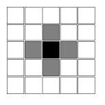
Figure 1: Different neighbourhoods for Cellular Automata: (a) von Neumann neighbourhood, (b) Moore neighbourhood, (c) extended Moore neighbourhood and (d) neighbourhood mediated by the Moore parameter $\pi_{M}$

These types of neighbourhood are illustrated in figure 1. The neighbourhood type and the number of cell states determine the number of rules one has to specify (in principle). For a neighbourhood of $N$ cells and $s$ possible cell states one needs $s^{N+1}$ rules. (This means, for example, $2^{9}=512$ for a two-state model on a 2D grid with Moore neighbourhood as for example Conway’s Game of Life.)

Therefore in many models, the updates rules depend only on the number of neigbours in a certain state, but not on their actual position. This of course greatly simplifies the speficication of update rules.

When doing this, an interesting type of rules are those that use an extended neighbourhood (at least Moore-type), but reduce the importance of non-adjacent cells for the update. For update rules that only depend on the number of neigbours in a certain state, their number $N$ can be redefined as

$$N:=N_{\mathrm{adj}}+\pi_{M}\cdot N_{\mathrm{non-adj}}$$ (1)

where $N_{\mathrm{adj}}$ denotes the number of adjacent and $N_{\mathrm{non-adj}}$ the number of non-adjacent cells that are nevertheless regarded as neighbours. In case of the next-nearest-neighbours, the Moore parameter $\pi_{M}$ mediates the transition from a pure von Neumann neighbourhood ($\pi_{M}=0$) to a full Moore neighbourhood ($\pi_{M}=1$). The accordingly modified neighbourhood is also sketched in figure 1. Models of this kind have been studied in this paper, and the influence of $\pi_{M}$ on certain results has been checked.

3 The Forest Fire Model

Our model is a variation of wide-spread forest fire models (see [BCT:1990, CBJ:1990, clar-1994, honecker-1996-229, clar-1996-8, XToys96, grassberger-2002], which can also be re-interpreted as a disease-spreading model. In this article, however, the vocabulary will be mostly the one of living, burning and burnt-out trees.

3.1 Definition of the Model

The forest fire simulation takes place on a quadratic two-dimensional grid (in all the following simulations $128\times 128$) with periodic boundary conditions and a mediated Moore neighbourhood as described in section 2. The states were encoded the following way:

$x$	colour	state of tree
$-1$	black	dead (burnt-out) tree
$0$	white	empty cell (or fire-resistant tree)
$1$	green	living tree
$2$	red	burning tree

The only possible transitions are those from living to burning state, $[1\to 2]$, and those from the burning state to the burnt-out one, $[2\to(-1)]$. The probability that a living tree at $(i,\,j)$ catches fire is given by:

$$p_{[1\to 2]}\left(i,\,j,\,t\,|\;\mathcal{N}_{t-1}\right)=\delta_{x_{i,\,j},\,1}\cdot\left\{1-(1-p_{b})^{N_{b,t-1}}\right\}$$ (2)

where $p_{b}$ denotes a fixed burning probability. The state of the cell’s neighbourhood at the previous timestep is symbolized by the condition complex $\mathcal{N}_{t-1}$, it explicitly enters the formula as $N_{b,t-1}$, the number of burning neighbours at $(t-1)$,

$$N_{b,\,t-1}=\left[\sum_{\begin{array}[]{c}\scriptstyle\Delta_{i,j}\in\{-1,0,1\}\\ \scriptstyle|\Delta_{i}|+|\Delta_{j}|=1\end{array}}\delta_{x_{i+\Delta_{i},\,j+\Delta_{j}},2}\quad+\quad\pi_{M}\cdot\sum_{\begin{array}[]{c}\scriptstyle\Delta_{i,j}\in\{-1,0,1\}\\ \scriptstyle|\Delta_{i}|+|\Delta_{j}|=2\end{array}}\delta_{x_{i+\Delta_{j},\,j+\Delta_{j}},2}\right]_{t-1}.$$ (3)

A burning tree is converted to a burnt-out one after one timestep, formally

$$p_{[2\to-1]}\left(i,\,j,\,t\,|\;\mathcal{N}_{t-1}\right)=\delta_{x_{i,\,j},\,2}$$ (4)

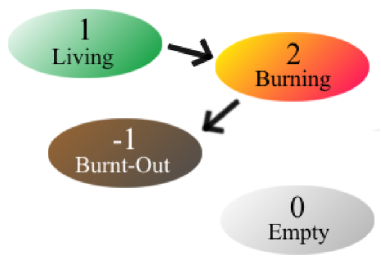
Figure 2: (a) Sketch of the basic forest fire model (b) Expamples for weak, drastic and critical decreases of the number of burning trees in a smoothed time series

A symbolic sketch of the model is given in figure 2.a. Equation (2) together with the definition of $N_{b,\,t-1}$ expresses the increased probability of a tree catching fire if it has more than one burning neighbour. In the case $N_{b,\,t-1}=1$ the probability reduces to

$$p_{[1\to 2]}\left(x_{i,\,j},t\,|\,\mathcal{N}_{t-1}\right)=\delta_{x_{i,\,j},\,1}\cdot\left\{1-(1-p_{b})\right\}=\delta_{x_{i,\,j},\,1}\cdot p_{b}$$ (5)

3.2 A Typical Simulation Run

At the beginning of the simulation, living trees are placed with a density $d_{\mathrm{start}}\in[0,1]$ while the remaining cells stay empty. Than a few number of burning trees are inserted – starting with only one burning tree would dramatically increase the probability of a ”false start”.

An example of a typical simulation run is shown in figure 3 for the choice $p_{b}=d_{\mathrm{start}}=0.63$. Even some runs with varied parameters already indicate that there is a relatively sharp “phase transition” between those configurations where the fire dies out within a few steps and those where almost the whole forest is affected.

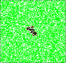
Figure 3: Snapshots of a forest fire simulation and corresponding time series of burning trees (critical case, $p_{b}=d_{\mathrm{start}}=0.63$)

This is shown in figure 4 where the end configurations of different characteristic simulations runs are given. There is indeed an analogy to phase transitions in physical systems – for example the Ising (see figure 5, taken from [GuEvIsin98]).

(a)	(b)	(c)

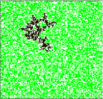
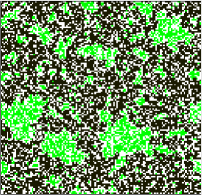
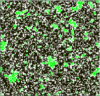
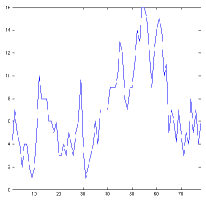
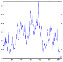
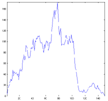
Figure 4: Typical end configuration and time series of burning trees in forest fire simulations: (a) subcritical case ($p_{b}=d_{\mathrm{start}}=0.60$), (b) critical case ($p_{b}=d_{\mathrm{start}}=0.63$) and (c) supercritical case ($p_{b}=d_{\mathrm{start}}=0.66$). Note the different timescales, in particular the fact that in case (b) the fire lasts about twice as long as in case (c).

In the Ising model, for temperatures below $T_{c}\approx 2.268254878$ the system is quite homogeneous (ordered with only small fluctuations). It is quite homogeneous as well for temperatures significantly above $T_{c}$ (disordered with only small correlated regions). At $T=T_{c}$, however, the picture is drastically different: There are clusters on all length scales and the correlation length diverges. (For all simulations on a finite grid, the correlation length cannot diverge; thus the picture of clusters at all length scales remains also true for $T\approx T_{c}$.)

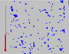
Figure 5: Snapshots of simulations of the Ising model for subcritical case ($T<T_{c}$), critical case ($T=T_{c}$) and supercritical case ($T>T_{c}$)

Analogously we denote cases where the fire dies out within a few timesteps and leaves behind a homogenous, almost unaffected system as subcritical, as illustrated in 4.a. A situation as depicted in figure 4.b where one finds burnt and unaffected clusters at all length scales is classified as critical. If, as depicted in figure 4.c, the fire affects the whole system and leaves behind again a homogeneous system of burnt tree we denote this as supercritical.

3.3 Relation to Other Models

In contrast to the majority of the models mentioned in the introduction to section 3, our model does not exhibit self-organized criticality. For example in the Clar-Drossel-Schwabl-model [clar-1994] the combination of a growth process and repeated ignition of forest fires is believed to push the system into a critical state. From the exposition given in subsection 3.2 this is easy to understand on an intuitive level. As long as the system is in a subcritical state, fires will die out after a few timesteps, resulting in net growth. In a supercritical state, large clusters will burn, which yields net loss of trees. The combination of both mechanisms will lead to a critical quasi-equilibrium.

In our model no growth mechanism is present, so – as it is the case in typical statitical mechanics systems – parameters have to be fine-tuned to access a critical state. Accordingly this model provides a very close look at the bruning process of a cluster, a “magnifying glass” which allows to study certain properties of self-organized criticality whithout the need to be very close to the critical point. Otherwise the critical state is hard to access numerically, since in order to deal with diverging correlation lengths, huge grids are required to have finite-size effects under control.

As outlined in [Lichtenegger:2005DA] the main reason why this model has been studied is the fact that it can easily generalized to a semi-realistic disease-spreading model. A publication on that model is in preparation (see also comments in section 6).

4 Analysis Tools

After having performed the simulation (which is finished when there are no burning trees left), it is the main task to extract the essential information and to condense it to a small set of significant numbers that can be easily compared for various runs and different parameter configurations.

There are two sources of information that are easily available: the final tree configuration and the time series of burning trees (both depicted in figure 4). The main quantities which can be extracted from them are summarized in table 9.

4.1 Cluster Analysis

The methods covered in this section are in a way related both to determining the fractal dimension of geometric objects by box-counting and the ideas of the renormalization group [Wilson:1973jj], in particular when formulated in the language of block-spin transformations à la Kadanoff.

Starting point is a the end configuration after a simulation run, i.e. a lattice of cell states $S^{(0)}:=\{s_{i,\,j}\}$ (as they were defined in equation (3): $s=-1$ for a burnt-out, $s=0$ for an empty and $s=1$ for a living cell). Now multiple cells are combined to new one,

$$s_{i,\,j}^{\prime}=f\left(s_{i_{ij,1},\,j_{ij,1}},s_{i_{ij,2},\,j_{ij,2}},s_{i_{ij,3},\,j_{ij,3}},\ldots,s_{i_{ij,k},\,j_{ij,k}}\right),$$ (6)

a procedure that yields a smaller lattice of new cells with states $S^{(1)}=\{s_{i,\,j}^{\prime}\}$. This process can of course be repeated, resulting in a sequence of lattice configurations:

$$\left(S^{(0)},\,S^{(1)},\,S^{(2)},\ldots,S^{(\Omega)}\right).$$

where $S^{(\Omega)}$ is a lattice consistent of too few cells to repeat the procedure defined in equation (6). Here, four cells were combined to a new one via

$$s_{i,\,j}^{\prime}=\mathrm{sign}\,\left(s_{2i-1,\,2j-1}+s_{2i-1,\,2j}+s_{2i,\,2j-1}+s_{2i,\,2j}\right)$$ (7)

a process which is illustrated in figure 6. Of course, other procedures are possible as well, and others are necessary to treat models with other types of states.

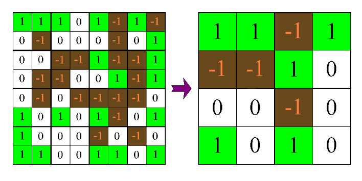
Figure 6: Combining cells as described in equation (7)

A suitably chosen characteristic observable $O(n)$ can be evaluated for each of these configurations,

$$O(n)=O(S^{(n)}),$$ (8)

and its values may give insight to the typical length scales present in the system. On this behalf, one can try to fit an analytic function $O(x)$ to them and read off a the size distribution of clusters. The most obvious choice for $O$ is

$$O(n)=\frac{1}{N_{n}}\sum_{s_{i,\,j}\in S^{(n)}}s_{i,\,j}$$ (9)

(with $N_{n}$ denoting the total number of cells in a configuration $S^{(n)}$) which was employed here, but alternatives for $O$ are possible as well.

Of course, after a sufficient number of recombination steps, in most cases values of $+1$ or $-1$ will remain. The first case corresponds to the scenario where the fire has stopped after a comparatively small number of timesteps (subcritical), the second is valid for mostly burnt-out trees (supercritical). In both cases, also in view of well-known results on fractal respectively box-counting dimensions, $O(n)$ from equation (9) can reasonably be approximated by an exponential function:

$$f(n)=1-e^{-\alpha_{e}n}$$ (10)

for dominance of $+1$, respectively

$$f(n)=-1+e^{-\alpha_{e}n}$$ (11)

in the case of $-1$ dominating. The constant $\alpha_{e}$ here is a measure of cluster size: When $\alpha_{e}$ is small, this means that there are also larger clusters of opposite cell state; a large value of $\alpha_{e}$ indicates rapid “saturation” and therefore the existence only of small clusters.

In the critical case, however, living and burnt-out trees are equally present in the whole simulation region, so this results in values of zero repeatedly emerging on all length scales during the combination process, and so the exponential fit often fails.

So in addition, also a linear (least-square) fit has been performed. Of course, in most cases, a linear function is only a rather poor description – but it is reliable in the sense that there is a straightforward way to find the fit and one always has a result (more or less meaningful). So in addition to $\alpha_{e}$ from equation 10 respectively 11, also a parameter $\alpha_{l}$ for a fit

$$f(n)=\alpha_{l}\,n+C$$ (12)

has been retrieved. Both parameters usually show the same qualitative behaviour. (An important exception for $p_{b}\to 1$ is discussed in section 5.1.)

For the critical case the cluster size distribution is expected to obeye a power-law; while this issue has been left to further investigation (which has to be performed on much larger grids and to be compared with results for SOC models mentioned in section 3), a sign for an arising power-law ist the fact that in the critical case an exponential fit (10, 11) becomes unstable and often breaks down completely.

4.2 Time Series Analysis

Information can also be retrieved from the time series of burning trees. Examples for such a time series are given in figures 3, 4, 7 and 8. There is number of meaningful and interesting quantities that can be extracted from such a time series by rather simple means. Some other parts of the analysis done, however, rely on more sophisticated techniques, namely discrete Fourier transform (see section 4.3).

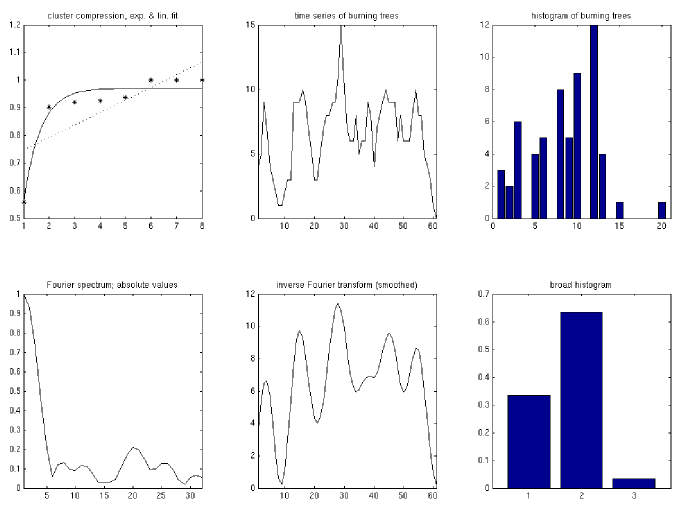
Figure 7: Time series and cluster analysis for typical runs of forest fire simulations ($N=128$): (a) subcritical case ($p_{b}=d_{\mathrm{start}}=0.61$), (b) supercritical case ($p_{b}=d_{\mathrm{start}}=0.66$). In each case, the results of exponential and linear fit to cluster compression (equations 10 and 11), the time series of burning trees, a corresponding histogram, the Fourier transform, a smoothed version of the time series and at last a very rough histogram are shown.

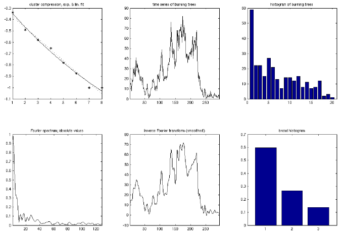
Figure 8: Time series and cluster analysis for two critical forest fire simulation runs ($N=128$, $p_{b}=d_{\mathrm{start}}=0.63$). As in figure 7, exponential and linear cluster fit, the time series of burning trees, the Fourier transform, a smoothed time series and two histograms are given. In (b), however, the exponential fit (as a tool for cluster analysis) fails.

Some characteristic numbers can be read off from the time series without problems: the total burning time $t_{\mathrm{burn}}$ (timesteps from the first tree catching fire to the last one becoming burnt-out) and the maximum number of burning trees $N_{\mathrm{burn,max}}$. The three main cases (subcritical, critical and supercritical) are shown in figure 4 (where one should mind the different scales, both for time and number of burning trees). The corresponding time series is in all cases quite characteristic:

• In the subcritical case, the fire only affects a small fraction of the system. In the strongly subcritical region, it is extinguished after a few timesteps, but for parameters approaching the critical region, it may last much longer. However, at any timestep the number of burning trees is comparatively small. There is of course at least one maximum, but there may be several of them, in any way they tend to be not significant.

• In the critical case, the progression of the fire is far more complicated than in the other cases. Large unaffected clusters may form (and sometimes be partially consumed later by the fire). The maximum number of burning trees is smaller than in the supercritical case (but significantly higher than the subcritical values). Due to this and to the emerging cluster structure, the fire tends to last longer (up to approximately the double supercritical burning time).

• In the supercritical case, all but a few trees are destroyed by the fire. Since the fire propagates nearly with maximum speed, it dies off soon after the whole system has been affected. There may be some small clusters, separated from the bulk, that allow the fire to survive some steps longer, but nevertheless there is usually a significant maximum and in virtually any case a rapid decrease (as, for example, in figure 7). In the supercritical limit ($p_{b}\to 1$, $d_{\mathrm{start}}\to 1$), the time series approaches a sawtooth with a clear maximum, and a sudden decrease to zero one or two steps later.

Also the fraction of burnt trees $f_{\mathrm{burn}}$ can easily be calculated. In this special case, it is simply the sum over the whole time series, divided by the initial number of trees. Again, in the subcritical case, $f_{\mathrm{burn}}$ will be small, in the supercritical it will approach one, and for the critical case there will be a wide range of possible values – even for the same set of parameters.

Possibly $t_{\mathrm{burn}}$ is the best value to indicate the phase transition from sub- to supercritical configuration. When starting subcritical and then slowly increasing $p_{b}$ and/or $d_{\mathrm{start}}$, one will notice a dramatic increase in $t_{\mathrm{burn}}$ when reaching the critical region and a significant decrease when leaving it towards supercriticality. (This is discussed in more detail in section 5.1.)

Also $N_{\mathrm{burn,max}}$ and $f_{\mathrm{burn}}$ are possible indicators for the transition, but since they usually monotonically increase on the path from sub- to supercriticality, it may be harder to identify the phase transition when watching these quantities.

Another sort of information can be extracted from histograms. Figures 7 and 8 also include two histograms each – one with 20 bins and one with only three bins. So the second one contains three characteristic numbers $h_{0}$, $h_{1}$ and $h_{2}$ which give the fraction of timesteps when there were comparatively few, medium or many burning trees.

A quantity that may become quite interesting as well, is the number of dramatic decreases of the number of burning trees – but due to the rather noisy nature of the time series this information is relatively hard to extract from the original series. So it is postponed to the next section which deals with Fourier analysis.

4.3 Fourier Analysis

From the time series one can deduce the Fourier spectrum as well. This has been done with the MATLAB^(R) FFT routine (using Fast Fourier Transform). The Fourier transform is also displayed in figures 7 and 8. In all cases, low frequencies dominate the spectrum (which is already clear from the shape of the time series).

In addition there tend to be several other peaks that represent higher frequencies modulating the signal; for very high frequencies, these peaks drown in noise. So on the one hand, the positions and intensities of such peaks (or at least the most important one) may characterize some aspects of the time series.

On the other hand, by cutting off the noisy high-frequency part of the spectrum and transforming back, one has a smoothed version of the time series (as also shown in figures 7 and 8). From this modified time series, for example the number of decreases can be read off.

These decreases have been separated in weak (less than $25\%$), drastic ($25\%$ to $50\%$) and critical (more than $50\%$) ones, and the counts of the latter two have been regarded as significant for the fire spreading. Of course there will be at least one dramatic decrease (when the fires finally dies off), which is trivial and is therefore not counted here. Especially in the case of critical fire propagation, there tend to be several more such decreases. (See for example figure 2.b.)

The appearence of drastic and critical decreases seems to characterize critical behaviour quite well, since it is more or less absent in sub- or supercritical simulation data. This can also be understood from the characteristics of critical fire propagation: On the edge between affecting most cells and dying off soon, there are repeatedly situations when only a few burning trees are left and those when a whole cluster catches fire. When smoothing out the time series, setting the cutoff point usually requires some fine-tuning (and it of course may affect all results).

For the Fourier analysis presented in section 5 the method described so far has been slightly modified: In order to increase the comparability of results, short time series have been expanded to a length of $2^{8}=256$ steps (by adding zeros after the simulation data). So one can establish a more unified scale for the Fourier transform.

From there, all but the lowest $32$ frequencies have been cut from the spectrum (that contained initially $\frac{1}{2}\cdot 2^{8}=128$ frequencies). While this choice is of course arbitrary, it yields trustworthy results that mostly coincide with those put forth by the best instrument for such types of analysis – human eye and brain.

$Q$	meaning	sec.
$f_{\mathrm{burn}}$	fraction of burnt trees (burning rate)	4.2
$t_{\mathrm{burn}}$	total burning time	4.2
$N_{\mathrm{burn,max}}$	maximum number of burning trees	4.2
$\alpha_{e}$	exponential fit parameter from cluster analysis	4.1
$\alpha_{l}$	linear fit parameter from cluster analysis	4.1
$h_{0}$	fraction of steps with ”few”
	($\in[0,\,\frac{N_{\mathrm{burn,max}}}{3}]$) burning trees	4.2
$h_{1}$	fraction of steps with ”several”
	($\in(\frac{N_{\mathrm{burn,max}}}{3},\,\frac{2N_{\mathrm{burn,max}}}{3}]$) burning trees	4.2
$h_{2}$	fraction of steps with ”many”
	($\in(\frac{2N_{\mathrm{burn,max}}}{3},\,N_{\mathrm{burn,max}}]$) burning trees	4.2
$\nu_{D}$	frequency of dominant Fourier peak	4.3
$I_{D}$	intensity of peak at $\nu_{D}$	4.3
$n_{\mathrm{dras}}$	number of drastic decreases ($25\%$ to $50\%$)	4.3
$n_{\mathrm{crit}}$	number of critical decreases ($>50\%$)	4.3

Figure 9: Summary of the quantities $Q$ eventually used as indicators of the fire propagation (and especially the phase transition). “sec.” denotes the section where the appropriate quantity is explained in detail

5 Results

Here some fundamental results are presented. In contrast to the few (but nevertheless characteristic) examples presented so far, now the complete parameter space of the model has been scanned systematically.

Since there are only two parameters that strongly influence system behaviour (namely $p_{b}$ and $d_{\mathrm{start}}$) such a scan is possible with moderate computational effort and the results can be displayed in a $2D$-plot.

The grid size has little influence on any result (as long as the lattice is sufficiently large, so that the initially burning trees incur no significant bias and subcritical propagation affects only a small fraction of the system). So we used a $128\times 128$ cell grid for all simulations.

The Moore parameter $\pi_{M}$ has greater influence on the result, in section 5.2 however, we will demonstrate that while there are quantitative changes, the qualitative behaviour is not modified. So all other simulations have been performed with $\pi_{M}=0.5$.

The parameters $p_{b}$ and $d_{\mathrm{start}}$ have been varied from zero to one in steps of $\Delta p_{b}=\Delta d_{\mathrm{start}}=0.01$, for each configuration there have been $40$ simulation runs where the quantities given in section 4 have been extracted.

Both mean values (indicated by a bar, as for example in $\overline{t_{\mathrm{burn}}}$) and standard deviations (here indicated by a capital delta, $\Delta$) of these quantities are, for all configurations, given in figure 10.

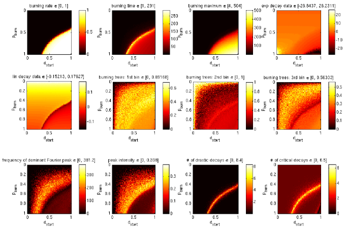
Figure 10: Significant system characteristics for $p_{b}=0:.01:1$, $d_{\mathrm{start}}=0:.01:1$ and 40 iterations: (a) mean values, (b) corresponding deviations. The quantities displayed are from left to right (i) in the first row burning rate $f_{\rm burn}$, total burning time $t_{\rm burn}$, maximum number of burning trees $N_{\rm burn,max}$ and exponential decay constant $\alpha_{e}$, (ii) in the second row the linear decay constant $\alpha_{l}$ and the histogram values $h_{1}$, $h_{2}$, $h_{3}$, (iii) in the third row the frequence $\nu_{D}$ of the dominant peak, its intensity $I_{D}$, the number $n_{\rm dras}$ of drastic and $n_{\rm crit}$ of critical decreases.

5.1 The Phase Transition

As it has already been mentioned, the model exhibits a (surprisingly sharp) ”phase” transition between two radically different kinds a behaviour, referred to as subcritical and supercritical, as described in section 4.2. On most plots in figure 10.a, the transition line is clearly to be seen.

This line is approximately a hyperbola with $p_{b}\cdot d_{\mathrm{start}}\approx C=\mathrm{const}$ where we have the $C\approx 0.4$ for the constant. While the hyperbola is at least no bad approximation for the transition line, the true form can not be deduced from the given data – it may even have a fractal substructure. Its width, however, does not exceed a few percent of change in both parameters (and probably it is still widened due to finite size effects and the limited amount of data given.)

The burning rate $f_{\mathrm{burn}}$ increases from below $10\%$ to above $90\%$ on this line. On the same line in configuration space, the total burning time $t_{\mathrm{burn}}$ reaches its maximum value, decreasing both towards the sub- and the supercritical region. The burning maximum $\overline{N_{\mathrm{burn,max}}}$ begins to increase from significantly below $100$ to more than $200$, but this transition is not that sharp and there is a further increase up to about $\overline{N_{\mathrm{burn,max}}}=500$ for $p_{b}\to 1$ and $d_{\mathrm{start}}\to 1$.

For the exponential decay parameter $\alpha_{e}$ there seems to be no clear transition at all, this impression, however, is created only by the plot scales. Since there are both regions with $\overline{\alpha_{e}}>25$ (for $d_{\mathrm{start}}\ll 1$ and $(1-p_{b})\ll 1$) and $\overline{\alpha_{e}}<-25$ (for $(1-d_{\mathrm{start}})\ll 1$ and $(1-p_{b})\ll 1$), the line of $\overline{\alpha_{e}}\approx 0$ that indicates the transition is hardly visible.

Since the range of values is more limited for $\alpha_{l}$, the phase transition is easier to recognize for this fit parameter. The transition again has $\overline{\alpha_{l}}\approx 0$, but now, such values are also reached for $p_{b}\to 1$, in region where $\overline{\alpha_{e}}$ takes its extreme values. This, however, is clear from the nature of the different fits. In these regions, the exponential decay is very fast, so already from the second step on, the data points lie approximately on a straight horizontal line, and therefore we have $\alpha_{l}\approx 0$.

The histogram data ($h_{0}$ to $h_{2}$) is more difficult to interpret. Also in these plots, the transition line is visible, but it is only one of several regions where interesting changes occur. Also for frequency and intensity of the Fourier spectrum, the interpretation is not that easy. For the product $p_{b}\cdot d_{\mathrm{start}}$ being small (i.e. $\ll 1$), one has a low maximum intensity at a low frequency. This can be accounted to a very short time series, yielding only a few frequencies. (The following zeros affect the scaling, but not the frequencies present in the signal.)

With $p_{b}$ and/or $d_{\mathrm{start}}$ increasing, first frequency and intensity of the peak tend to increase, indicating a signal fluctuating an a small scale. Near the critical line, however, there is a significant decrease in mean peak frequency, indicating modulation of the signal on much larger scale. This is also consistent with the increase of the number of drastic or critical decreases – one often has several times when the fire has nearly died off, but also periods of chain-reaction-like propagation.

These results (especially when interpreting the model as one of disease propagation) are in a way unsettling: Even an small change of either population density or susceptibility may introduce the transition from an isolated (endemic) disease to an epidemic or even pandemic one. Especially a decrease in resistance can easily be induced by natural catastrophes or starvation – the black death in Europe from 1347 to 1353 or the Spanish influenza after world war I are likely to be interpreted this way.

On the other hand, they also indicate that even small changes (in population density as well as in susceptibility) can reduce an epidemic diseases to a mere nuisance. However, one should be cautious when transferring the results of such models to systems which they are not intended to be described (as it is human society).

5.2 Influence of the Moore parameter $\pi_{M}$

As defined in 2, the Moore parameter $\pi_{M}$ is a way to formally mediate the transition from a von Neumann to a Moore neighbourhood. In the previous simulations, $\pi_{M}=0.5$ has been employed. Now we study the effects of changing $\pi_{M}$.

Therefore simulations as described in 5.1 have been performed for $\pi_{M}=0$ (pure von Neumann neighbourhood) and $\pi_{M}=1$ (full Moore neighbourhood). The results are given in figure 11.

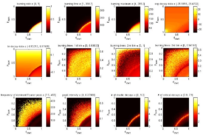
Figure 11: Results of changing the Moore parameter: (a) $\pi_{M}=0$, (b) $\pi_{M}=1$; ($p_{b}=0:.01:1$, $d_{\mathrm{start}}=0:.01:1$, 10 iterations each). The quantities displayed are the same as in figure 10 except that only mean values, not deviations are shown.

As it is also the case in figure 10, there is a clear phase transition (indicated especially by $f_{\mathrm{burn}}$, $t_{\mathrm{burn}}$ and $\alpha_{l}$), but the transition line is shifted – towards a larger product $p_{b}\cdot d_{\mathrm{start}}$ for $\pi_{M}=0$, towards a smaller $p_{b}\cdot d_{\mathrm{start}}$ for $\pi_{M}=1$. (This result is fully consistent with what could be expected, since a higher $\pi_{M}$ results in a higher fire propagation probability.)

Since the behaviour is qualitatively the same for all choices of $\pi_{M}$, it seems justified to perform this type of simulation with just one value for the Moore parameter (where we have used $\pi_{M}=0.5$).

5.3 Individual Susceptibilities

While the model presented here is of course limited in its range of applications, there is nevertheless a simple modification that can be implemented with virtually no additional effort – the substitution of a global burning probability by an individually varying one.

So we define a matrix $\mathbf{P}$ with elements $p_{i,j}$ that describe the individual burning probabilities of the cells $(i,\,j)$ and replace equation (2) by

$$p_{[1\to 2]}\left(i,\,j,\,t\,|\;\mathcal{N}_{t-1}\right)=\delta_{s_{i,j},1}\cdot\left\{1-(1-p_{i,j})^{N_{\mathrm{burn},t-1}}\right\}$$ (13)

The distribution of the elements $p_{i,j}$ can in principle be chosen arbitrarily, but it seems reasonable to pick them from a Gaussian distribution centered at $p_{b}$:

$$p_{i,j}=\mathrm{med}\left\{0,\,G(p_{b};\,\sigma_{b}),\,1\right\}=\mathrm{med}\left\{0,\,p_{b}+\sigma_{b}\,G(0;\,1),\,1\right\}$$ (14)

with $\mathrm{med}$ denoting the median value and $G(\mu;\,\sigma)$ a random variable from a Gaussian distribution with mean $\mu$ and variance $\sigma$. For $\sigma_{b}=0$ this is exactly the model already studied, but for $\sigma_{b}\neq 0$ (where we use without loss of generality $\sigma_{b}>0$) new effects may arise. So we studied the various cases; the results for a distribution ($\sigma_{b}=0.1$) and a broad distribution ($\sigma_{b}=0.5$) are displayed in figure 12, and figure 13. (Compared to figures 10 and 11, the resolution of configuration space sampling has been reduced due to the computational cost.)

Qualitatively, there are no severe changes, although the phase transition line widens for higher values of $\sigma_{b}$. This seems clear, since a wide range of burning probabilities allows some sub- and supercritical configurations to obtain characteristics from the critical case. On the other hand, critical configurations may gain more characteristics of either sub- or supercriticality as well, so the transition is smeared out over a larger region of parameter space.

The magnitude of the standard deviation does not change significantly compared to simulations performed for $\sigma_{b}=0$ (but with otherwise identical parameters). This may be somehow surprising, since one could expect the deviation in $p_{\mathrm{burn}}$ to result in larger differences between simulation runs with the same choice of parameters.

But of course for the critical or nearly critical case, even with $\sigma_{b}=0$ the same set of parameters can lead to radically different outcomes. So the deviations can be expected to be large already in this case; any change of $\sigma_{b}$ will not significantly increase them. Nevertheless there are several significant quantitative changes because of the modification of the width $\sigma_{b}$:

• The burning rates $f_{\mathrm{burn}}$ are reduced in the supercritical region, which is clear since also in the supercritical case now there will remain several trees with a burning probability considerably lower than average.

• The total burning time $t_{\mathrm{burn}}$ is reduced as well as the burning maximum $N_{\mathrm{burn,max}}$, probably due to similar reasons.

• While the change in the linear fit parameter $\alpha_{l}$ is not significant, this is not true for the exponential fit via $\alpha_{e}$. Large values of $|\alpha_{e}|$ indicate a rapid saturation in the cell combination analysis – and such a saturation will definitely be slowed down by regions of considerably increased or reduced burning probability. So $|\alpha_{e}|$ is considerably smaller for larger values of $\sigma_{b}$.

• The dominant Fourier peak is shifted towards lower frequencies while the intensities remain similar.

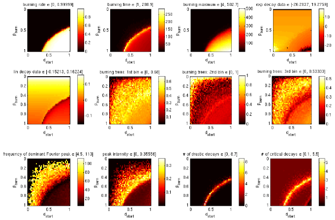
Figure 12: Influence of $\sigma_{b}=0.1$, simulations on a $128\times 128$-grid with $\pi_{M}=0.5$, $\Delta p_{b}=\Delta d_{\mathrm{start}}=0.025$ and 10 iterations: (a) data, (b) deviations. The quantities displayed are the same as in figure 10

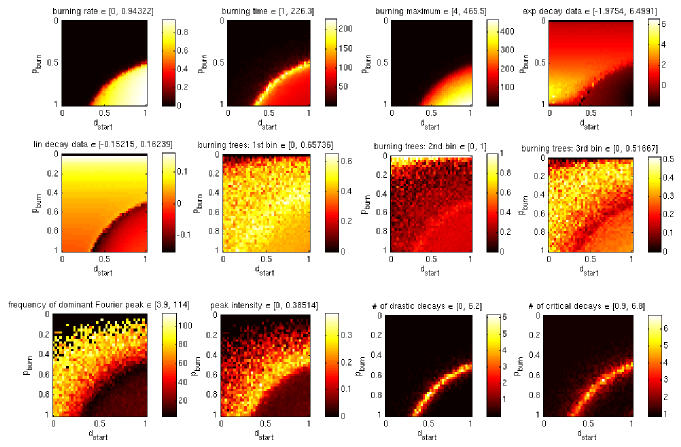
Figure 13: Influence of $\sigma_{b}=0.5$, simulations on a $128\times 128$-grid with $\pi_{M}=0.5$, $\Delta p_{b}=\Delta d_{\mathrm{start}}=0.025$ and 10 iterations: (a) data, (b) deviations. The quantities displayed are the same as in figure 10

6 Summary and Outlook

We have studied an enhanced forest fire model that shows a surprisingly sharp phase transition in respect to the two main parameters, namely tree density $d_{\mathrm{start}}$ and burning probability $p_{b}$ for a healthy tree with a burning neighbour.

In a large region of configuration space, the fire (or pathogen) vanishes within a few timesteps, whereas in most of the remaining space, the fire affects almost the whole population. The border between these two outcomes is a small region of “critical” behaviour that can be characterized by cluster formation (on any length scale) and exceptional values for many characteristic quantities. (For example the total burning time tends to be more than twice as long as in any other case.)

A redefinition of neighbourhood, controlled by the Moore-parameter $\pi_{M}$ did not change the qualitative behaviour, but influenced the position of the line of critical behaviour in phase space. In contrast, the transition to individual susceptibility had only small influence on the global characteristics of the system also on quantitative level.

The model can easily be re-interpreted as a disease spreading model, where susceptible, infected and removed individuals replace living, burning and burnt-out trees. Our results thus may indicate that the transition from an endemic disease (which can only affect a small fraction of the population) to an epidemic (or, depending on the system, even a pandemic) can be driven by a change of just a few percent in one crucial parameter.

While some analysis is to be done also for this model (like the check whether for the critical case a power law arises for the cluster size distribution), there are several possible extensions which remain to be investigated. Allowing empty cells to be (re)populated changes the model significantly and reduces the importance of the initial density. Some results can be found in [Lichtenegger:2005DA]; a comprehensive article on this topic is in preparation.

References

- [1] Von Neumann J. et Burks A. ed., Theory of Self-Reproduction Automata, University of Illinois Press, 1966, p. 77, in Ostolaza J.L., Bergareche A.M., La vie artificielle, Seuil, Paris, 1997, pp. 37-38.
-
[2]
Klaus Lichtenegger, Stochastic Cellular Automata
Models in Disease Spreading and Ecology,
diploma thesis, 2005; available on
http://physik.uni-graz.at/kll/cthesis.pdf - [3] M. L. Martins et al., Cellular automata model for citrus variegated chlorosis, Physical Review E, 62, 5, 2000
- [4] P. D. Morley, J. Chang, Critical Behavior in a Cellular Automata Animal Disease Transmission Model, arxiv.org/abs/physics/0308028, 2003
- [5] Hokky Situngkir, Epidemology Through Cellular Automata, Case of Study: Avian Influenza in Indonesia, delivered in open session of Board of Science, Bandung Fe Institute, January 29, http://cogprints.org/3500/, 2004
- [6] Maria Magdoń-Maksymowicz, Simulation of a Horizontal and Vertical Disease Spread in Population, in M. Bubak et al. (eds), ICCS 2004, LNCS 3039, p. 750-757, Springer-Verlag; Berlin, Heidelberg, 2004
- [7] Shih Ching Fu, George Milne, A Flexible Automata Model for Disease Simulation, in P.M.A. Sloot, B. Chopard, A.G. Hoekstra (eds), ACRI 2004, LNCS 3305, p. 642-649, Springer-Verlag; Berlin, Heidelberg, 2004
- [8] Siegfried Clar, Klaus Schenk, Franz Schwabl Phase Transitions in a Forest-Fire Model, Phys. Rev. E, 55, 2174, arXiv.org:cond-mat/9701062, 1997
- [9] G. J. Ackland, M. A. Clark, T. M. Lenton, Catastrophic desert formation in Daisyworld, Journal of Theoretical Biology, 223, p. 39-44, 2003
- [10] Bak, P., Chen, K. and Tang, C. (1990), A forest-fire model and some thoughts on turbulence, Phys. Lett. A 147, 297 300.
- [11] K. Chen, P. Bak, M. H. Jensen, A deterministic critical forest-fire model, Phys. Lett. A 149, 207 210, 1990
- [12] S. Clar, B. Drossel, F. Schwabl, Scaling laws and simulation results for the self-organized critical forest-fire model, arXiv.org:cond-mat/9405008, 1994
- [13] A. Honecker, I. Peschel, Critical Properties of the One-Dimensional Forest-Fire Model, PHYSICA A, 229, 478, arXiv.org:cond-mat/9511132, 1996
- [14] S. Clar, B. Drossel, F. Schwabl, Forest fires and other examples of self-organized criticality, COND.MAT. 8, 6803, arXiv.org:cond-mat/9610201, 1996
- [15] Michael Creutz, Xtoys: cellular automata on xwindows, Nuclear Physics B (Proc. Suppl.), 47, p. 846-849, http://thy.phy.bnl.gov/www/xtoys/xtoys.html, 1996
- [16] Peter Grassberger, Critical Behaviour of the Drossel-Schwabl Forest Fire Model, arXiv.org:cond-mat/0202022, 2002
- [17] S. Gürtler, H. G. Evertz, Simulation of Ising und XY-Model, Projekt Multimediale Lehre Technische Universität Graz, http://www.itp.tu-graz.ac.at/MML/isingxy/, 2002
- [18] K. G. Wilson and J. B. Kogut, The Renormalization group and the epsilon expansion, Phys. Rept. 12 (1974) 75.
- [19] D. Stauffer, A. Aharony, Introduction to Percolation Theory, Taylor and Francis, London, 2nd ed., 1992