Mass Accretion Rates and Histories of Dark Matter Haloes

Abstract

We use the extensive catalog of dark matter haloes from the Millennium simulation to investigate the statistics of the mass accretion histories (MAHs) and accretion rates of $\sim 500,000$ haloes from redshift $z=0$ to 6. We find only about 25% of the haloes to have MAHs that are well described by a 1-parameter exponential form. For the rest of the haloes, between 20% (Milky-Way mass) to 50% (cluster mass) experience late-time growth that is steeper than an exponential, whereas the remaining haloes show plateau-ed late-time growth that is shallower than an exponential. The haloes with slower late-time growth tend to reside in denser environments, suggesting that either tidal stripping or the “hotter” dynamics are suppressing the accretion rate of dark matter onto these haloes. These deviations from exponential growth are well fit by introducing a second parameter: $M(z)\propto(1+z)^{\beta}e^{-\gamma z}$. The full distribution of $\beta$ and $\gamma$ as a function of halo mass is provided. From the analytic form of $M(z)$, we obtain a simple formula for the mean accretion rate of dark matter, $\dot{M}$, as a function of redshift and mass. At $z=0$, this rate is $42M_{\odot}\,{\rm yr}^{-1}$ for $10^{12}M_{\odot}$ haloes, which corresponds to a mean baryon accretion rate of $\dot{M}_{b}=7M_{\odot}\,{\rm yr}^{-1}$. This mean rate increases approximately as $(1+z)^{1.5}$ at low $z$ and $(1+z)^{2.5}$ at high $z$, reaching $\dot{M}_{b}=27,69$, and 140 $M_{\odot}\,{\rm yr}^{-1}$ at $z=1$, 2, and 3. The specific rate depends on halo mass weakly: $\dot{M}/M\propto M^{0.127}$. Results for the broad distributions about the mean rates are also discussed.

1 Introduction

The mass growth history is a basic property of dark matter haloes. Haloes in numerical simulations are seen to be assembled through a number of processes: mergers with comparable mass haloes (“major mergers”), mergers with smaller satellite haloes (“minor mergers”), and accretion of non-halo material that is composed of either haloes below the numerical resolution or diffuse particles. Following the mass history of the most massive progenitor halo as a function of redshift $z$ is a useful way to quantify a halo’s mass assembly history. These mass accretion histories (MAHs, or $M(z)$) are important for statistical studies of the distributions of halo formation redshifts, and the correlations between formation time and other halo properties such as environment, concentration, substructure fraction, spin, and relative contributions to mass growth from major vs minor mergers. Moreover, the time derivative of the MAH gives the mass growth rate of dark matter haloes, which is directly related to the accretion rate of baryons from the cosmic web onto dark matter haloes.

A number of earlier papers have investigated various aspects of the halo MAHs. For instance, Wechsler et al. (2002) analyzed $\sim 900$ haloes (above $10^{12}h^{-1}M_{\odot}$ at $z=0$) in a $\Lambda$CDM simulation in a $60\,h^{-1}$ Mpc box with $256^{3}$ particles. The values from a 1-parameter fitting function for the MAHs were presented for 8 haloes. Clear correlations between the formation redshift $z_{f}$ and concentration $c$ of haloes were seen, with late-forming haloes being less concentrated. The scatter in $c$ was attributed to the scatter in $z_{f}$. An alternative 2-parameter fitting function was demonstrated by van den Bosch (2002) to be superior to a 1-parameter fit to haloes in a simulation with the same particle number in a $141h^{-1}$ Mpc box.

The relationship between halo structure and accretion was further addressed in Zhao et al. (2003) and Zhao et al. (2003), where the redshift dependence of $c$ was observed to be more complicated than a simple proportionality. Tasitsiomi et al. (2004) examined 14 haloes, ranging in mass from group to cluster scale (.58 to $2.5\times 10^{14}h^{-1}M_{\odot}$) and also found that a 2-parameter fit for $M(z)$ worked better. Cohn & White (2005) studied the mass accretion histories of $\sim 1500$ cluster-sized haloes and characterized several properties of galaxy cluster formation.

Maulbetsch et al. (2007) studied the environmental dependence of the formation of $\sim 4700$ galaxy-sized haloes (above $10^{11}h^{-1}M_{\odot}$) in a $50\,h^{-1}$ Mpc simulation box. In higher-density environments, they found the haloes to form earlier with a higher fraction of their final mass gained via major mergers. Li et al. (2008) studied 8 different definitions of halo formation time using the haloes from the Millennium simulation (Springel et al., 2005). The motivation was to search for halo formation definitions that better characterize the downsizing trend in star formation histories, as opposed to the hierarchical growth of haloes in the $\Lambda$CDM cosmology. Zhao et al. (2008) (Z08) investigated the mean MAH in different cosmological models – scale-free, $\Lambda$CDM, standard CDM, and open CDM – and searched for scaled mass and redshift variables that would lead to a universal fitting form for the median MAH for all models.

The results in these earlier papers were presented either for $M(z)$ of a handful of individual haloes, or for the global mean growth of a selection of haloes. Our aim here is to quantify systematically the diversity of growth histories and rates using the $\sim 500,000$ $z=0$ haloes with $M>10^{12}M_{\odot}$ (i.e. above 1000 simulation particles) and their progenitors in the Millennium simulation. Over this large range of haloes, we find that an exponential fit does not adequately capture the behavior of halo growth. Many haloes experience large changes in the rate at which they accrete mass. Some haloes grow more slowly at late times, and occasionally even lose mass, while other haloes undergo late bursts of growth. All of these MAHs are poorly fit by an exponential, and suggest the need for a fitting form with more flexibility. We find it helpful to classify the MAHs into four types based on their late-time accretion rate. The large ensemble of haloes allows us to quantify the mean values as well as the dispersions of the mass accretion rates and halo formation redshifts as a function of mass and redshift.

This paper is organized as follows. Sec. 2 provides some background information about the haloes in the Millennium simulation and describes how we construct halo merger trees. This post-processing of the Millennium public data is necessary for identifying the thickest branch (i.e. the most massive progenitor) along each final halo’s past history. The masses of these progenitors will then allow us to quantify the MAH, $M(z)$. In Sec. 3, we first assess the accuracy of the 1-parameter exponential form for $M(z)$. We then propose a more accurate two-parameter function for $M(z)$ and classify the diverse assembly histories into four broad types according to their late-time growth behavior. We further quantify the statistics of the two fitting parameters, providing (in the Appendix) algebraic fits for their joint distributions that can be used to generate Monte Carlo realizations of an ensemble of halo growth tracks. The applicability of $M(z)$, which is derived for $z=0$ haloes, for the mass accretion history of higher-redshift haloes is discussed in Sec. 3.3. Sec. 4 is focused on the statistics of the mass accretion rates. A simple analytic expression is obtained for the mean accretion rate, $\left<\dot{M}\right>$, of dark matter as a function of halo mass and redshift. The dispersions about the mean rates are significant, as evidenced by the differential and cumulative distributions of $\dot{M}$ presented here. Sec. 5 discusses the mean and the distribution of the halo formation redshift as a function of halo mass. In Sec. 6 we report the correlations of MAHs with halo environment, the last major merger redshift, and the fraction of haloes’ final masses assembled via different types of mergers.

2 Halo Merger Trees in the Millennium Simulation

The Millennium simulation (Springel et al., 2005) provides a database for the evolution of roughly $2\times 10^{7}$ $z=0$ dark matter haloes from redshifts as high as $z=127$ in a $500h^{-1}$ Mpc box using $2160^{3}$ particles of mass $1.2\times 10^{9}M_{\odot}$ (all masses quoted in this paper are in units of $M_{\odot}$ and not $h^{-1}M_{\odot}$). It assumes a $\Lambda$CDM model with $\Omega_{m}=0.25$, $\Omega_{b}=0.045$, $\Omega_{\Lambda}=0.75$, $h=0.73$, and a spectral index of $n=1$ for the density perturbation power spectrum with a normalization of $\sigma_{8}=0.9$.

Dark matter haloes are identified with a friends-of-friends (FOF) group finder (Davis et al., 1985) with a linking length of $b=0.2$. Throughout this paper we use the number of particles linked by the FOF finder to define the halo’s mass. Once identified, each FOF halo is then broken into gravitationally bound substructures (subhaloes) by the SUBFIND algorithm (see Springel et al. 2001). These subhaloes are connected across the 64 available redshift outputs: a subhalo is the descendant of a subhalo at the preceding output if it hosts the largest number of the progenitor’s bound particles. The resulting subhalo merger tree can be used to construct merger trees of FOF haloes, although we have discussed at length in Fakhouri & Ma (2008, 2009) the complications due to halo fragmentation and have presented comparisons of several post-processing algorithms that handle fragmentation events.

Our results in this paper are based on the stitch-3 post-processing algorithm described in Fakhouri & Ma (2008). In this algorithm, fragmented haloes that remerge within 3 outputs after fragmentation are stitched into a single FOF descendant; those that do not remerge within 3 outputs are snipped and become orphan haloes. After applying the stitch-3 algorithm, we extract the mass accretion history, $M(z)$, of each halo at $z=0$ (or at any higher redshift) by following the halo’s main branch of progenitors. We have compared the resulting $M(z)$ and formation redshifts to those obtained from the alternative algorithms (e.g., “snip,” “split,” and subhalo vs FOF mass) discussed in Fakhouri & Ma (2008, 2009). We find the systematic variations to all be within 5-10% of the stitch-3 values of these quantities.

3 Fitting Mass Accretion Histories

3.1 Previous MAH Forms

To quantify the limitations of the exponential fit in capturing halo growth, consider the formation redshift $z_{f}$, here defined as the redshift at which $M(z)$ is equal to $M_{0}/2$.

For the 1-parameter exponential form (e.g. Wechsler et al. 2002)

$$M(z)=M_{0}e^{-\alpha z},$$ (1)

the parameter $\alpha$ is simply related to $z_{f}$ by

$$z_{f}=\frac{\ln(2)}{\alpha}.$$ (2)

We have compared $z_{f}$ as determined by the exponential fit to each halo’s $M(z)$ from the simulation with the $z_{f}$ determined directly from the $M(z)$ tracks such that $M(z_{f})=M(0)/2$ (using interpolation between output redshifts). We find the exponential fit to err systematically in its determination of $z_{f}$, significantly overestimating the formation redshift for haloes that form recently and underestimating it for haloes that form early. The mean value of $z_{f}$ from the exponential fit, for instance, is 0.3 higher than the actual value for young haloes and is 0.8 lower for old haloes across all masses.

A more complicated functional representation of MAHs was put forth by van den Bosch (2002):

$$\log\left(\frac{M(z)}{M_{0}}\right)=-0.301\left[\frac{\log(1+z)}{\log(1+z_{f})}\right]^{\nu},$$ (3)

where $\nu$ and $z_{f}$ are fitting parameters. The use of an additional parameter provided significant improvement in the quality of the fits for many MAHs, especially those that formed late. This 2-parameter form, however, is not flexible enough to handle haloes that have lost mass, as it cannot take on values that would give $M(z)/M_{0}$ greater than 1. Moreover, over the sample of haloes tested in van den Bosch (2002), comparison between the goodness-of-fit of this two-parameter form and the exponential fit showed that the exponential fit actually performs better for early forming haloes.

3.2 A Revised MAH Form

To address the need for a fit that is both effective and simple, we find a 2-parameter function of the form

$$M(z)=M_{0}(1+z)^{\beta}e^{-\gamma z},$$ (4)

to be versatile enough to accurately capture the main features of most MAHs in the Millennium Simulation. This form has also been studied in Tasitsiomi et al. (2004) for cluster-mass haloes, but it has not been tested over a large number of haloes of different mass. The form reduces to an exponential when $\beta$ is 0, and $\gamma$ in this case is simply the inverse of the formation redshift: $\gamma=\ln(2)/z_{f}$. A large fraction of the haloes, however, are better fit when the additional factor of $(1+z)^{\beta}$ in equation (4) is included. In general, $\beta$ can be either positive or negative, but $\gamma\geq 0$. We find the combination $\beta-\gamma$ to be a useful parameter for characterizing these MAHs as $\beta-\gamma$ gives the mass growth rate at small redshifts:

$$\frac{d\ln(M(z))}{dz}=\frac{\beta}{1+z}-\gamma\approx\beta-\gamma+{\cal O}(z)\,.$$ (5)

This late-time trend can be used to characterize the MAH as described below.

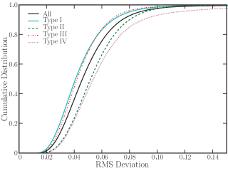
Figure 1: Cumulative distribution for the RMS deviations between the fitting formula eq. (4) and the Millennium Nbody output for the mass growths of 478,781 $z=0$ haloes (solid black) and the four sub-types (colored curves) listed in Table 1. The figure shows that the fits perform well overall: about 75% of the haloes have RMS deviations less than $\sim 6$%.

To obtain the best-fit values for $\beta$ and $\gamma$ in equation (4), we have performed a $\chi^{2}$-like minimization of the quantity

$$\Delta^{2}=\frac{1}{N}\sum_{N}\frac{[M(z_{i})/M_{0}-(1+z_{i})^{\beta}e^{-\gamma z_{i}}]^{2}}{M(z_{i})/M_{0}}\,,$$ (6)

where the sum is over the $N$-available simulation redshift outputs at $z_{i}(i=1,...,N)$ for each halo. The choice of the factor $M(z_{i})$ in the denominator is akin to assuming Poissonian errors for halo masses. We found this choice to be a suitable middle ground between minimizing simply the sum of squares and minimizing the fractional deviation (i.e. with a factor of $M^{2}(z)$ in the denominator). The former tended to fit the finely sampled low-$z$ points well at the expense of the sparsely spaced high-$z$ points, whereas the latter tended to do the opposite. Equation (6), on other hand, provides reasonable fits for the entire history of the halo growth. Fig. 1 shows the cumulative distribution for the rms deviation of the fits from the Nbody data (normalized by $M_{0}$) for all $\sim 500,000$ $z=0$ haloes. The deviation is less than 6% for over 75% of the haloes, and only a few percent of haloes have deviations larger than 10%. Of this most poorly fit subset of haloes, nearly half underwent mass loss at late times. As expected, the fits become progressively worse at higher redshifts; for over 75% of haloes, the maximum fractional deviation between the fits and Nbody results occurs above $z=4$.

Type	Criteria	Characteristics	$\frac{\chi^{2}_{1}}{\chi^{2}_{2}}$
I	$|\beta|$ $<$ 0.35	Good exponential	$1.09$
II	$\beta-\gamma<$ -0.45	Steep late growth	$1.61$
III	-0.45 $<\beta-\gamma<$ 0	Shallow late growth	$2.15$
IV	$\beta-\gamma>$ 0	Late plateau/decline	$3.31$

Table 1: MAHs are categorized based upon the best fit parameters $\beta$ and $\gamma$ of equation (4). Categorization is done in order by type; thus MAHs that satisfy the criteria for both Type I and Type II belong to Type I. The right-most column is the mean of $\chi^{2}_{1}/\chi^{2}_{2}$, the ratio of the $\chi^{2}$ computed for the 1-parameter exponential form to the $\chi^{2}$ computed for the 2-parameter form in equation (4). Values $>1$ imply that the 2-parameter form provides a more accurate fit than the 1-parameter form.

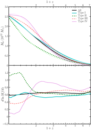
Figure 2: Average mass accretion histories (top) and their derivatives (bottom) for the total population (black solid) and the four types of halo growths listed in Table 1. The average is taken over the $M(z)$ for galaxy-sized haloes with masses between $2.1\times 10^{12}M_{\sun}$ and $3.3\times 10^{12}M_{\sun}$ in the Millennium simulation, although haloes at different mass show similar behavior. In the top panel, the set of curves with the lighter shading shows the average $M(z)$ computed from our fits of equation (4) to each halo’s MAH. The bottom panel illustrates that the late-type growth rates differ greatly, ranging from $d\ln M/dz\sim 1.2$ for Type II to 0.1 for Type IV.

We suggest that the parameters $\beta$ and $\gamma$ allow for rough classifications of MAHs into a few basic groups, summarized in Table 1. The classification scheme is quite straightforward. Fits with small values for $\beta$ indicate a weak contribution from the $(1+z)$ term, and deviate minimally from an exponential curve. These haloes with $|\beta|<0.35$ are labeled Type I.

The rest of the classifications are dependent upon the value of $\beta-\gamma$. The motivation for this is the fact that the difference represents the value of the derivative at $z=0$, as noted in equation (5). Hence Type II haloes, defined to be those haloes with $\beta-\gamma<-0.45$, feature steep growth at late times, typically steeper than can be captured by an exponential fit.

Type III haloes have fit parameters that fall in the range $-0.45<\beta-\gamma<0$ and exhibit flat late time growth. Like Type II, these tend to deviate from the fit that would be found using the exponential form, but Type III haloes do so in the opposite direction to Type II haloes. A typical Type III halo has undergone limited growth during recent times, sometimes after a spurt of growth at earlier times.

Type IV, with $\beta-\gamma>0$, represents the most extreme deviation from an exponential. The majority of Type IV haloes have shed mass, some of them by significant amounts. Some Type IV haloes have merely seen their growth slow down like the Type III haloes, but over a more significant period of time. As such, Type IV haloes are extreme cases of Type III haloes, perhaps representing the future growth for some Type III haloes.

The boundaries delineating these classifications are rough guidelines at best. For example, consider the definition for Type I of $|\beta|<0.35$. For the largest values of $\beta$ in this group, which should be considered the worst of the “good exponentials” that constitute Type I, the fractional difference between the formation redshift as determined by the simple exponential and the modified exponential is a little under 8%. The agreement is not perfect, but the two fits are similar enough for these haloes that the use of the power law parameter adds little. Of course, there is no reason why we should not instead demand that the formation redshifts differ on average by no more than 5%, or perhaps 10%. In the end, the combination of the formation redshift metric and a couple of others for comparing the fits suggested that demanding $|\beta|<0.35$ was inclusive enough to capture the majority of haloes for which an exponential is an adequate fit, without unduly diminishing the integrity of the group.

Fig. 2 compares the shapes of the average MAH for haloes of galaxy-size mass from the Millennium simulation for the overall distribution and for each type. The bottom panel shows the derivative $d\ln M/dz$ to highlight the different late-time accretion rates among the four types. Haloes of other mass show similar behavior. Clearly, the late time growth rate is an important factor in distinguishing haloes from one another. The average MAH for Type I haloes is quite similar to that of the overall distribution, which indicates that the average MAH is approximately exponential. However, the behavior of about 75% of individual haloes deviates from an exponential noticeably. This fact is quantified in the right-most column of Table 1, where the ratio of $\chi^{2}$ for the exponential fit to the 2-parameter fit is seen to increase with the MAH types.

Since the mean MAH is approximately exponential, the accretion rate $d\ln M/dz$ averaged over the whole population is also nearly independent of redshift (black solid curves in Fig. 2) when expressed in units of per redshift, with $d\ln M/dz$ being between 0.6 and 0.7 for $z=0$ up to 5. This weak dependence on redshift is similar to that of the halo merger rates (per unit $z$) reported in Fakhouri & Ma (2008). The different types of haloes, however, show significant dispersions in the late-time accretion rates, with $d\ln M/dz$ being as high as 1.2 for Type II and as low as 0.1 for Type IV at $z\approx 0$.

For each of the mean profiles shown in Fig. 2, we have fit the analytic form in equation (4). The best-fit values of $(\beta,\gamma)$ are (0.10, 0.69) for all haloes, and ($-0.04$, 0.54), ($-0.9$, 0.35), (0.62, 0.88), and (1.42, 1.39) for each of the four types, respectively.

Mass Range	Halo Number	Type I	II	III	IV
($10^{12}M_{\odot}$)
1.2 to 2.1	191421	29%	27%	32%	12%
2.1 to 4.5	143356	27%	29%	32%	12%
4.5 to 14	95744	24%	34%	31%	11%
14 to 110	43089	20%	42%	26%	11%
$>110$	4787	18%	57%	17%	8%
	478781	27%	31%	31%	11%

Table 2: Within each mass range, the percentage of haloes that belong to each type are provided. For each type, there is a noticeable trend with mass, though the strength of the trend varies.

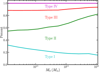
Figure 3: Cumulative fraction of haloes belonging to a given MAH type as a function of halo mass (e.g. the magenta type-IV curve includes the contributions from the three other types). The exponential form (Type I) is a good fit for only 20% to 30% of the haloes at all masses. The type II fraction shows a strong mass dependence, reaching $\sim 60$% for cluster-mass haloes.

The statistics of the 478,781 $z=0$ haloes (above 1000 particles, or a mass of $1.2\times 10^{12}M_{\odot}$) belonging to each MAH type across different mass bins are given in Table 2 and Fig. 3. Exponential MAH (Type I) is seen to apply to only 20 to 30% of the haloes. There is also interesting dependence of the type on halo mass. Most notably, Type II haloes feature a strong dependence on mass, where the fraction rises from 27% at $\sim 10^{12}M_{\odot}$ to 60% at $\ga 10^{14}M_{\odot}$. Cluster-size haloes therefore not only form late, which is a natural consequence of the $\Lambda$CDM cosmology, but the majority of their mass accretion rates is also faster than an exponential at low redshifts.

The results presented thus far are for the mean MAH and mean values of $(\beta,\gamma)$. We find, however, significant dispersions about the mean behavior that are also important to characterize. For completeness, we show the distributions of our best-fit $(\beta,\gamma)$ for all halo MAHs in the Appendix and Fig. 12. We also present there an accurate fitting form that we have obtained for the two-dimensional probability distribution of $\beta$ and $\gamma$ as a function of halo mass. This formula can be used to generate a Monte Carlo ensemble of realistic halo growth histories. The details of the formula, its usage, and comparison to the Millennium data are described in the Appendix. We emphasize that the results presented for the rest of this paper are obtained from the Millennium haloes directly rather than from this Monte Carlo realization.

3.3 MAHs for Haloes at Higher Redshifts

The MAHs presented thus far are obtained from the main branches of the descendant haloes at $z=0$. Thus, for a higher redshift $z_{1}>0$, the distribution of $M(z_{1})$ contains only information about the main branch progenitors, which is a subset of all the haloes at $z_{1}$ since many haloes do not belong to main branches.

Since the formation of higher-redshift galaxies and their host haloes is of much interest, it is useful to quantify the behavior of MAHs for haloes at $z_{1}$, where $z_{1}>0$. In particular, we ask whether the mean MAH for haloes of mass $M_{1}$ at $z_{1}$ for $z>z_{1}$ can be related to the MAHs of haloes at $z=0$ that we have studied thus far.

We find that the mean MAH of haloes of mass $M_{1}$ at $z_{1}$ is nearly identical to the mean MAH of haloes at $z=0$ that satisfy $M(z_{1})=M_{1}$. That is, the mean MAH for $z>z_{1}$ of the main branch subset with mean mass $M(z_{1})=M_{1}$ at $z_{1}$ is very similar to the mean MAH of the complete population of haloes with mean mass $M_{1}$ at $z_{1}$. As a specific example, the mean MAH of the $10^{13}M_{\odot}$ $z=0$ haloes in the simulations had the value $M(z=1)=4.5\times 10^{12}M_{\odot}$ at $z=1$. We find that the mean MAH of these $10^{13}M_{\odot}$ haloes at $z>1$ is nearly identical (within 2%) to the $z>1$ evolution of the mean MAH of all $M_{1}=4.5\times 10^{12}M_{\odot}$ haloes at $z=1$. This property for the mean MAH is in fact a natural consequence of the Markovian nature of the Extended Press-Schechter theory (see, e.g., Sec 2.3 of White 1994).

This self-similar property implies that in order to study the MAH properties of haloes with mass $M_{1}$ at redshift $z_{1}$, one simply needs to determine which set of haloes at $z=0$ have $M(z_{1})=M_{1}$. In particular, one needs to compute the average mass $M_{0}$ of the haloes at $z=0$ that map onto $M(z_{1})=M_{1}$ at $z_{1}$. This mapping is shown in Fig. 4 with $M_{1}$ along the x-axis and $M_{0}$ along the y-axis for $z_{1}=0,0.5,1,$ and $2$. Note that $M_{0}=M_{1}$ at $z_{1}=0$ by construction, and as $z_{1}$ increases, the mass $M_{0}$ that maps onto some fixed $M_{1}$ by redshift $z_{1}$ also increases.

We note that the mapping in Fig. 4 implies that haloes of some mass $M_{1}$ at some redshift $z_{1}>0$ do not have the same shape of MAH as haloes of mass $M_{0}=M_{1}$ at $z=0$. That is, the MAH of a $10^{13}M_{\odot}$ halo at $z=0$ and the MAH of a $10^{13}M_{\odot}$ halo at $z_{1}>0$ are not simply related by a shift from $z$ to $z-z_{1}$ in equation (4). This is because haloes at higher $z_{1}$ have a relative formation redshift $z_{f}-z_{1}$ that is smaller than haloes of the same mass at $z=0$. This result is not surprising since haloes of the same mass at different redshifts in the $\Lambda$CDM model represent different part of the mass spectrum and are not generally expected to have identical properties.

We have tested the self-similar property of the fitting form of Z08 (using their online code) by comparing their mean MAH for $z=0$ $10^{13}M_{\odot}$ haloes and the MAH for their $M(z=1)$ haloes at $z>1$. Their latter MAH is higher than the former by about 15%, while ours differ by less than 2%.

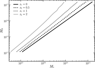
Figure 4: For haloes of mass $M_{1}$ at redshift $z_{1}$, the y-axis plots their corresponding mean mass $M_{0}$ today. Four values of $z_{1}$ are shown: 0 (solid), 0.5 (dashed), 1 (dot dashed), and 2 (dotted). This mapping allows one to use equation (4) for the MAH of higher-redshift haloes (see text).

4 Mass Accretion Rates: Mean and Dispersion

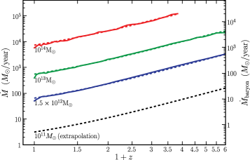
Figure 5: Mean mass accretion rate of dark matter as a function of redshift at halo mass $10^{11},1.5\times 10^{12},10^{13}$ and $10^{14}M_{\odot}$. The solid curves are computed from the Millennium haloes (except $10^{11}M_{\odot}$, which falls below our resolution limit of 1000 particles per halo) at a given mass ($\pm 20\%$ range); the dashed curves show the accurate fit provided by eq. (8). The right side of the vertical axis labels the mean accretion rate of baryons, $\dot{M}_{b}$, assuming a cosmic baryon-to-dark matter ratio of $\sim 1/6$. The slight dip in $\dot{M}$ at $z=0$ is due to the artificial edge effect inherent in the stitch-3 algorithm used to process the FOF merger trees.

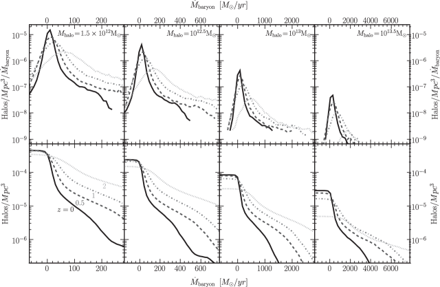
Figure 6: Differential (top) and cumulative (bottom) distributions of the accretion rates of cosmic baryons, $\dot{M}_{b}$, for four halo masses (left to right). Within each panel, the accretion rates at four redshifts $z=0$ (solid), 0.5 (dashed), 1 (dashed dotted), and 2 (dotted) are shown, where the distributions are seen to broaden significantly with increasing $z$. The vertical axis labels the number of haloes per comoving Mpc³ at or above a given $\dot{M}_{b}$.

Having quantified $M(z)$ in Sec. 3, we now examine its time derivative – the mass accretion rate – in more detail. In particular, we would like to obtain a general formula for the mean accretion rates of dark matter for a wide range of halo mass and redshift. To achieve this, we note that our analytical form in equation (4) for individual halo MAHs gives:

$$\frac{\dot{M}}{M}=0.10h\,{\rm Gyr}^{-1}\left[\gamma(1+z)-\beta\right]\sqrt{\Omega_{m}(1+z)^{3}+\Omega_{\Lambda}}$$ (7)

where $\Omega_{m}$ and $\Omega_{\Lambda}$ are the present-day density parameters in matter and the cosmological constant, and we have assumed $\Omega_{m}+\Omega_{\Lambda}=1$ (used in the Millennium simulation) and matter-dominated era in computing $dz/dt$. As shown in Sec. 3, the parameters $\beta$ and $\gamma$ in equation (7) generally depend on the halo mass. We find, however, that the mass dependence follows a simple power law independent of the redshift, and the simple analytic form in equation (7) provides an excellent approximation for the mean mass accretion rate as a function of redshift and halo mass:

$$\left<\dot{M}\right> = 42\,M_{\odot}{\rm yr}^{-1}\left(\frac{M}{10^{12}M_{\odot}}\right)^{1.127}$$ (8)

$$\times(1+1.17z)\sqrt{\Omega_{m}(1+z)^{3}+\Omega_{\Lambda}}\,.$$

For completeness, the best fit for the median growth rate computed in the Millennium simulation is

$$\left<\dot{M}\right>_{\rm median} = 24.1\,M_{\odot}{\rm yr}^{-1}\left(\frac{M}{10^{12}M_{\odot}}\right)^{1.094}$$ (9)

$$\times(1+1.75z)\sqrt{\Omega_{m}(1+z)^{3}+\Omega_{\Lambda}}\,.$$

We note that the overall amplitude of the mean is higher than the median due to the long, positive, $\dot{M}$ tail (see Fig. 6).

Fig. 5 compares the mean accretion rates of dark matter in $M_{\odot}$ per year computed from the Millennium simulation (solid curves) and this formula (dashed curves) for haloes of mass $10^{12}M_{\odot}$ to $10^{15}M_{\odot}$ over the redshift range of 0 and 5. The overall trend of the accretion rate is such that $\dot{M}/M$ has a weak dependence on $M$ ($\propto M^{0.127}$), and its dependence on redshift is approximately $(1+z)^{1.5}$ at low $z$ and $(1+z)^{2.5}$ at $z>1$. This $z$-dependence is motivated by our 2-parameter form for $M(z)$ and is more accurate than the simple power law used in Genel et al. (2008), Neistein et al. (2006), and Neistein & Dekel (2008); our $z\sim 0$ value, on the other hand, is consistent with theirs to within 20%. We have also computed $\dot{M}$ from the fitting form for the median MAH in the recent preprint by Z08. We found their $\dot{M}$ to have a slightly steeper $z$-dependence than our equation 9 where their median value is within 20% of our median $\dot{M}$ at $z\sim 0$ but exceeds ours by a factor of $\sim 2$ at $z\sim 4$.

Along the right side of the vertical axis of Fig. 5, we label the corresponding mean accretion rates of baryons, $\dot{M}_{b}$, assuming a cosmic baryon-to-dark matter ratio of $\Omega_{b}/\Omega_{m}\approx 1/6$. The results shown should be a reasonable approximation for the mean rate of baryon mass that is being accreted at the virial radius of a dark matter halo of a given mass. Fig. 5 and equation (8) indicate that this rate is $\dot{M}_{b}\approx 7\,M_{\odot}{\rm yr}^{-1}$ for $10^{12}M_{\odot}$ haloes today, and it increases to 27, 69, and 140 $M_{\odot}{\rm yr}^{-1}$ for $10^{12}M_{\odot}$ haloes at $z=1$, 2, and 3, respectively. Since the infalling baryons are a reservoir for the gas that fuels star formation, it is interesting to compare $\dot{M}_{b}$ with the mean star formation rates of different types of galaxies, e.g., $\dot{M}_{*}\sim 4M_{\odot}{\rm yr}^{-1}$ for the Milky Way (e.g., Diehl et al. 2006), suggesting that about half of the infalling $\dot{M}_{b}\approx 7\,M_{\odot}{\rm yr}^{-1}$ for Galactic-size haloes needs to be converted into stars. The relations among these different accretion rates and the implications will be investigated in a subsequent work.

Having determined the mean rates, we show their distributions and dispersions in Fig. 6. Four redshifts, $z=0$, 0.5, 1, and 2, and four ranges of halo masses (left to right panel) are shown. Both the differential (top panels) and cumulative (bottom panels) distributions of $\dot{M}_{b}$ are plotted for comparison. Within each panel, the distribution of $\dot{M}_{b}$ at a given halo mass is seen to broaden significantly with increasing redshift. For instance, the (comoving) number density of $1.5\times 10^{12}M_{\odot}$ haloes with $\dot{M}_{b}>250M_{\odot}$ yr^-1 increases dramatically from $5\times 10^{-7}$ Mpc^-3 at $z=0$ to $5\times 10^{-5}$ Mpc^-3 at $z=2$. At a given redshift, the distribution of $\dot{M}_{b}$ also broadens with increasing halo mass, although the distribution (and dispersion) of the ratio $\dot{M}_{b}/M_{b}$ is largely independent of mass. The latter is similar to the weak mass dependence of the mean $\dot{M}/M$ given by equation (8).

5 Formation Redshifts: Mean and Dispersion

It is well established that on average, more massive haloes form later than less massive haloes in the $\Lambda$CDM cosmology. The Millennium database provides sufficient statistics for us to quantify the distributions of the formation redshift $z_{f}$ and its mean and scatter over a wide range of halo masses ($\sim 10^{12}$ to $\sim 10^{15}M_{\odot}$). The formation redshift, along with the late-time growth rate $\beta-\gamma$, can be thought of as two physically motivated quantities parameterizing the halo MAH.

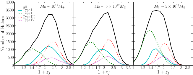
Figure 7: Distributions of the formation redshift $z_{f}$ for three mass bins (left to right). Within each mass bin, the $z_{f}$ distribution for all haloes is plotted (solid black), as well as the distribution for each halo type. While the relative amplitudes of the distributions do change from one mass bin to another, the overall shapes remain similar across all masses.

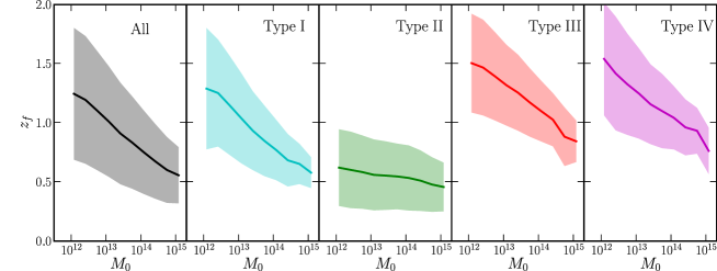
Figure 8: Mass dependence of the mean (solid curves) and one standard deviation scatter (shaded regions) of the formation redshifts of the Millennium haloes. More massive haloes on average form more recently, but the scatter is large. One exception is Type II haloes that have a mean $z_{f}$ of $\approx 0.5$ independent of mass. Fits to the mean and scatter of $z_{f}$ as a function of mass are given in Table 3.

	$z_{f}$ vs. $M_{0}$		$\gamma-\beta$ vs. $M_{0}$
	$\left<z_{f}\right>$	$\sigma_{z_{f}}$	$\left<\gamma-\beta\right>$	$\sigma_{(\gamma-\beta)}$
Overall	$-0.24x+1.26$	$-0.11x+0.58$	$-0.25x-0.29$	$0.14x+0.64$
Type I	$-0.25x+1.30$	$-0.12x+0.51$	$-0.22x-0.45$	$0.03x+0.21$
Type II	$-0.05x+0.62$	$-0.04x+0.34$	$-0.12x-1.15$	$0.14x+0.60$
Type III	$-0.23x+1.56$	$-0.08x+0.43$	$-0.03x-0.20$	$0.01x+0.11$
Type IV	$-0.23x+1.56$	$-0.08x+0.43$	$0.03x+0.15$	0.36

Table 3: Linear fits for the mass dependence of the mean formation redshift $z_{f}$, mean $\gamma-\beta$, and their respective 1$\sigma$ scatter about the mean, where $x\equiv\log_{10}(M_{0}/10^{12}M_{\sun})$.

The distributions of $z_{f}$ for each type of MAHs for three halo mass bins are plotted in Fig. 7. The overall trend of decreasing $z_{f}$ with increasing halo mass is evident across the three panels. Within each panel, a correlation between $z_{f}$ and the MAH type is clearly seen. Nearly all haloes in the smallest few $z_{f}$ bins are Type II. This means that despite the fact that Type II dominates the highest mass bins, the haloes that constitute Type II are not merely the especially massive haloes which formed late, but also include less massive haloes which formed late. On average, a Type II halo has a formation redshift 0.5 smaller than a typical halo. To a lesser degree, Type III and Type IV are also distinct from the overall distribution. Both tend to form early, Type III more so than Type IV, and together the two types account for most of the haloes that formed early.

Fig. 8 shows the mean formation redshift $z_{f}$ as a function of halo mass for all 478,781 $z=0$ Millennium haloes (leftmost panel) as well as for each type of MAH. As the scatter about the line is, to a good approximation, Gaussian, the 1$\sigma$ range about the line is also provided in the plots in each panel (light shaded areas). From these shaded areas, it is clear that there is considerable scatter for the overall distribution. The relationship between $M_{0}$ and $z_{f}$ is different from the overall distribution for all types except Type I, which suggests that the types discriminate by formation redshift to some extent. Also note that the separation of haloes into types also produces more limited scatter about the mean.

To approximate the mass dependence of the mean and scatter of $z_{f}$, we use the linear form

$$\left<z_{f}\right>=a\log_{10}\frac{M_{0}}{10^{12}M_{\odot}}+b\,,\quad\sigma_{z_{f}}=c\log_{10}\frac{M_{0}}{10^{12}M_{\odot}}+d$$ (10)

and find it to fit the simulation data accurately. Table 3 lists the best-fit coefficients for all the halo MAHs (above 1000 particles at $z=0$) and for each of the four types of MAHs shown in Fig. 8. Table 3 also includes the same fit performed for the fit parameters ($\beta-\gamma$). The mean formation redshifts differ significantly among the types, with $\left<z_{f}\right>\approx 0.6,1.3$, and 1.5 for Type II, I, and III (plus IV), respectively, for galaxy-size haloes. The dependence of $\left<z_{f}\right>$ on mass is noticeably weak for Type II; the other types show similar mass dependence, where $d\left<z_{f}\right>/d\log M$ ranges from $-0.23$ to $-0.25$.

With the relationships between formation redshift and mass for each type, we can look at how these dependences relate to the basic halo characteristics given in Table 1. Recall that Type II haloes were marked by steep growth at late times, which is captured by the very negative value of $\beta-\gamma$. Type III haloes, on the other hand, have small values for $\beta-\gamma$, and thus grow slowly at late times. The relationships shown in Fig. 8 are then no surprise. Type II haloes are also associated with late formation times, while Type III haloes tend to have formed quite early.

6 Correlations with Halo Environments and Major Merger Frequencies

Thus far we have discussed how the halo MAHs and mass accretion rates vary with halo mass and redshift. We have also shown that the mean $z_{f}$ depends on halo mass strongly, but the scatter in $z_{f}$ does not depend strongly on the MAH type nor halo mass. In this section, we investigate if the mean and scatter in $z_{f}$ are correlated with quantities other than halo mass. In particular, we ask if the shapes of MAHs (1) differ systematically between underdense vs overdense regions, and (2) are correlated with the time and frequency of major mergers and mass brought in by these events during a halo’s lifetime.

6.1 Environment

An extensive discussion and tests of halo environments can be found in Fakhouri & Ma (2009). Four definitions of a halo’s local environment based on the local mass density centered at the halo were compared. Three of them were computed using the dark matter particles in a sphere of radius $R$ centered at a halo, either with or without the central region carved out; the fourth definition was computed using the masses of only the haloes rather than all the dark matter. Here we use $\delta_{R-{\rm FOF}}$, computed by subtracting out the FOF mass $M$ of the central halo within a sphere of radius $R$:

$$\delta_{R-{\rm FOF}}\equiv\delta_{R}-\frac{M}{V_{R}\bar{\rho}_{m}}\,,$$ (11)

where $V_{R}$ is the volume of a sphere of radius $R$, and $\delta_{R}$ is the mean mass overdensity within $R$. This measure makes no assumption about the central halo’s shape. By taking out the mass of the central halo itself, this density was shown to be a more robust measure of the environment outside of a halo’s virial radius. Otherwise, the halo mass itself dominates the density centered at massive haloes (see Fig. 1 of Fakhouri & Ma 2009), and it becomes difficult to distinguish whether any correlations are due to the mass or the larger-scale environment in which the halo resides.

Fig. 9 shows the distribution of the environmental densities (evaluated at $z=0$) for haloes within each MAH type and the total population. The distribution for Type IV haloes is quite distinct from all other distributions and is offset towards higher densities. Since Type IV haloes experience very little mass growth or even mass loss at late times, denser environments appear to impede mass accretion onto haloes.

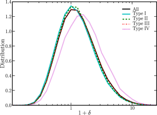
Figure 9: Normalized distributions in $\delta$ are plotted for all haloes, as well as each type of halo. The most prominent feature is the clear separation between Type IV and all other types. The center of the Type IV is well to the right of the other types, meaning that Type IV haloes are predominantly found in denser environments than any other type.

6.2 Mass Growth due to Major Mergers

Major mergers are more rare than minor mergers, but they can contribute to a significant fraction of a halo’s final mass, and have a strong impact on halo structures and galaxy properties such as the star formation rate.

A useful quantity for assessing the role of major mergers on halo MAHs is $z_{lmm}$, the redshift of the last major merger in a halo’s history. Fig. 10 shows the fraction of haloes whose last major merger occurred at or before $z$. Type II haloes are seen to experience a major merger in the much more recent past than the other types: about 65% of them had encountered a major merger within redshifts 0 and 0.3, and only 25% of them had their last major merger before $z=1$. In sharp contrast, only about 5% of Type III and IV haloes had a major merger later than $z=0.3$, and over 75% of them had their last major merger earlier than $z=1$.

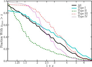
Figure 10: Distribution of the redshift of the last merger major for the four types of haloes (colored curves) and all $z=0$ haloes (solid black). The majority of the $z=0$ haloes with Type II MAH (dashed green curve) have experienced a major merger (of mass ratio $>0.33$) very recently, whereas the last major merger occurred earlier than $z=1$ for more than 75% of Type III and IV haloes.

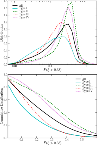
Figure 11: Differential (top) and cumulative (bottom) distributions of the fraction of halo mass gained from major mergers of mass ratio $\xi>0.33$. Much like the $z_{f}$ distributions, each Type is quite distinct from the overall distribution. Type I and III haloes feature few major mergers, while Type II and Type IV haloes tend to be dominated by major mergers. Type IV mergers also feature a noticeable rise in the highest bin, due to having gained more mass via major mergers across their history than they currently have.

Another useful parameter for quantifying the role of major mergers in its MAH is $F(\xi>\xi_{\rm min})$, which is the fraction of mass at $z_{0}$ that came from mergers above some progenitor mass ratio $\xi_{\rm min}$. We choose to define the mass ratio in relation to the mass of the progenitor at the time of merger, as opposed to being defined in relation to the halo’s present mass. The exact value of $F$ is strongly dependent upon the choice of $\xi_{\rm min}$. The overall features, however, do not change significantly, so different values for $\xi_{\rm min}$ only change the values for $F(\xi>\xi_{\rm min})$, but leave the overall characteristics in place.

Fig. 11 shows the differential (top) and cumulative (bottom) distribution of the major merger mass fraction, $F(\xi>0.33)$ for each type of MAHs. Type II haloes (dashed curves), which feature steep growth at late times, are seen to have the highest $F$ among the four types. The distribution peaks at $F\approx 0.4$, indicating that $\sim 40$% of their final mass was acquired through major mergers. Type I haloes (solid cyan curves), by contrast, feature a dearth of major mergers, which is unsurprising given the fact that large mergers are poorly handled by the simple exponential. Likewise, Type IV haloes (dotted curves), which grow quickly early on only to lose mass at late times, are dominated by major mergers with a number of Type IV haloes even having $F(\xi>\xi_{\rm min})>1$. This occurs when a halo has less mass presently than it has gained overall via major merger. Type III haloes (dotted dashed curves) tend to be relatively major merger free, which is again to be expected due to the decelerating growth of Type III haloes at later times during which much of the overall mass is accreted.

7 Conclusions

We have examined the mass growth histories of $\sim 500,000$ $z=0$ haloes and their progenitors in the Millennium simulation. The two-parameter function in equation (4) provides a reasonable fit for the MAHs of these haloes, as shown in Fig. 2. The mean mass accretion rate of dark matter (and baryons) as a function of halo mass and redshift is well approximated by equation (8), as shown in Fig. 5. The distributions of $\dot{M}$ are broad, and the number density of high-$\dot{M}$ haloes increases sharply with increasing $z$ at a given halo mass (see Fig. 6). The mean halo formation redshift as a function of mass is given by equation (10) and Fig. 8.

To facilitate the analysis of the halo MAH, we have classified $M(z)$ into four types based on their shapes. We have shown that only 20 to 30% of the Millennium haloes follow an exponential form (“Type I”) in their mass accretion history $M(z)$. Only one parameter is needed to specify their MAH, e.g., the formation redshift $z_{f}$. The formation redshift depends strongly on halo mass, as expected for hierarchical cosmological models such as the $\Lambda$CDM. The median $z_{f}$ ranges from 1.3 for $10^{12}M_{\odot}$ haloes to 0.6 for $10^{15}M_{\odot}$ haloes, and is dispersed over a range roughly equal to the median value for all masses.

About 20% of galaxy-size and 60% of cluster-size haloes have late-time growth that is steeper than an exponential (“Type II”). These haloes are formed more recently, with a median $z_{f}$ of about 0.5 for all masses. The redshift at which they experience the last major merger is also significantly later than the exponential haloes: about 50% of them have had the last major merger between $z=0$ and 0.3, as opposed to 10% of the rest of the haloes, including exponential haloes. Correspondingly, a higher fraction of Type II haloes’ final mass is acquired through major mergers, e.g. 60% of these haloes obtained more than 30% of their final mass from major mergers, whereas a little over 30% of all haloes obtained more than 30% of their final mass from major mergers, and fewer than 20% of exponential haloes did.

The rest of the haloes have stunted late-time growth relative to an exponential form. The median $z_{f}$ ranges from 1.5 at low mass to 0.8 at high mass. These haloes can be further separated into two groups (Type III and IV), where the two are primarily distinguished by the roles that major mergers have played in their growth; that is, Type III haloes tend to experience few major mergers, whereas Type IV haloes grew predominantly from major mergers at early redshifts. The MAHs of the two can be distinguished by the sharpness in the downturn of late time growth. Type IV haloes also live in somewhat denser environments, where the stronger tidal fields and more frequent interactions may have contributed to rapid accretion at early times followed by a slow down of their late time mass growth.

Despite this diverse behavior of halo MAHs, we have found the individual $M(z)$ to be well fit when a second parameter is introduced (eq. 4). To quantify the statistics of $M(z)$, we have provided fits to the joint probability distribution of the two MAH parameters $\beta$ and $\gamma$ in the Appendix. These can be used to generate realizations of halo mass growth histories in semi-analytic models of galaxy formation that incorporate realistic scatters about the mean trends.

Appendix A Joint Distribution of $\beta$ and $\gamma$

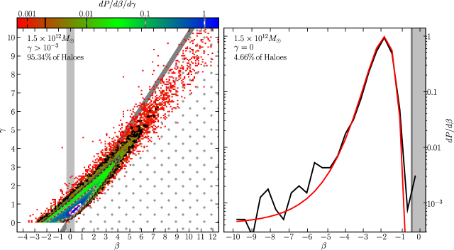
Figure 12: Probability distributions of $\beta$ and $\gamma$ for haloes of mass $1.5\times 10^{12}M_{\odot}$. The left panel is the PDF of $\beta$ and $\gamma$ for haloes with $\gamma>10^{-3}$ (95.34% of all haloes). The shaded 2D histogram presents the distribution of $\beta$ and $\gamma$ obtained from Millennium (see color scale for units) with corresponding contours drawn at the 0.005, 0.01,0.1 and 1 levels (black to white). The appropriately normalized fitting form $D_{2D}$ is overlaid as red dashed contour lines. The right panel is the PDF of $\beta$ for haloes with $\gamma=0$ (4.66%). The appropriately normalized fitting form $D_{1D}$ is overlaid in red. For both panels, the background shading corresponds to regions of phase space denote type I (grey), type II (red), type III (green) and type IV (blue) MAHs.

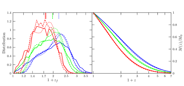
Figure 13: Distribution of the formation redshifts (left) and the mean MAHs (right) from the simulation directly (solid), the ($\beta,\gamma$) fits to the simulation MAHs (dashed), and a Monte Carlo ensemble of 300,000 halos per mass bin generated using equations (A1)-(A3) (dotted). In each panel, three mass bins are shown:$10^{12}M_{\odot}$ (blue), $10^{13}M_{\odot}$ (green), and $10^{14}M_{\odot}$ (red). Note that the dashed and dotted curves are almost indistinguishable in the right panel.

We have seen that halo MAHs are well-fit by equation (4) with two parameters $\beta$ and $\gamma$. Applying this fit to haloes in the Millennium simulation yields a joint distribution of $\beta$ and $\gamma$. In this appendix we provide a fitting form to this distribution as a function of $\beta$, $\gamma$, and halo mass that is intended to allow the reader to generate rapidly a mock catalog of MAH tracks. We find that a straightforward rejection method can generate 300,000 mock MAH trajectories in under a minute on a standard laptop. The mean properties of the resulting trajectories match the mean properties of the Millennium trajectories at the 10% level. The fitting forms presented below are chosen for the practical purpose of matching the underlying distribution as closely as possible.

We find that 95.34% of the haloes occupy a smooth region in the ($\beta,\gamma$) plane shown in the left panel of Fig. 12. The remaining 4.66% of the haloes live along a distinct line with $\gamma=0$ and $\beta\leq 0$, where the distribution of $\beta$ is shown in the right panel of Fig. 12. That is, their MAHs are better approximated by a power law in $1+z$ rather than an exponential. Interestingly, this 95.34% vs 4.66% division is independent of halo mass, even though the shape of the distributions generally depends on mass. For accuracy, we choose to separate the distribution of $\beta$ and $\gamma$ into these two components and fit to them separately.

For the 4.66% of haloes with $\gamma=0$, their $\beta$ distribution is well approximated by

$$\frac{dP}{d\beta}\propto e^{-X^{2}}$$ (12)

where

$$X=7.443\,e^{0.6335\beta+0.2626M^{0.1992}}-2.852M^{-0.05412}$$ (13)

and $M\equiv M_{\rm halo}/10^{12}M_{\odot}$. This fit is valid in the range $-10<\beta\leq 0$.

For the 95.34% of haloes with $\gamma>10^{-3}$, the joint distribution in $\beta$ and $\gamma$ is well approximated by

$$\frac{dP}{d\beta d\gamma}\propto e^{-(XM^{-0.05569})^{2}-(YM^{-0.05697})^{2}}$$ (14)

where

$$X = (-1.722-0.1568\beta+0.007592\beta^{2})(1-T_{2})+$$

$$(1.242+0.3138\beta-0.01399\beta^{2})T_{2}$$

$$Y = 13.39[1\!-\!1.224\tanh(1.043Y^{\prime})](1\!-\!0.08018\beta)$$

$$Y^{\prime} = \gamma-(28.85+0.4537\beta)(1-T_{1})-$$

$$(28.38+0.7624\beta)T_{1}+29.21M^{-0.001933}$$

$$T_{1} = 0.5[1+\tanh(1.174\beta)]$$

$$T_{2} = 0.5[1+\tanh(0.7671\beta-0.1269)]\,.$$

This is valid in the range $-8<\beta<12$, $0<Y^{\prime}<3$. Since the rejection method does not require a normalized PDF for input, we leave these probability distributions unnormalized.

Fig. 13 illustrates that Monte Carlo realizations generated from the probability distributions above (dotted curves) reproduce accurately the formation redshift distributions (left panel) and the mean MAHs (right panel) obtained from the $(\beta,\gamma)$ fits to the Millennium MAHs (dashed curves), and both match closely the results computed directly from the Millennium simulation (solid curves).

References

- Cohn & White (2005) Cohn J. D., White M., 2005, Astroparticle Physics, 24, 316
- Davis et al. (1985) Davis M., Efstathiou G., Frenk C. S., White S. D. M., 1985, ApJ, 292, 371
- Diehl et al. (2006) Diehl R., Halloin H., Kretschmer K., Lichti G. G., Schönfelder V., Strong A. W., von Kienlin A., Wang W., Jean P., Knödlseder J., Roques J.-P., Weidenspointner G., Schanne S., Hartmann D. H., Winkler C., Wunderer C., 2006, Nature, 439, 45
- Fakhouri & Ma (2008) Fakhouri O., Ma C.-P., 2008, MNRAS, 386, 577
- Fakhouri & Ma (2009) Fakhouri O., Ma C.-P., 2009, ArXiv e-prints
- Genel et al. (2008) Genel S., Genzel R., Bouché N., Sternberg A., Naab T., Schreiber N. M. F., Shapiro K. L., Tacconi L. J., Lutz D., Cresci G., Buschkamp P., Davies R. I., Hicks E. K. S., 2008, ApJ, 688, 789
- Li et al. (2008) Li Y., Mo H. J., Gao L., 2008, MNRAS, 389, 1419
- Maulbetsch et al. (2007) Maulbetsch C., Avila-Reese V., Colín P., Gottlöber S., Khalatyan A., Steinmetz M., 2007, ApJ, 654, 53
- Neistein & Dekel (2008) Neistein E., Dekel A., 2008, MNRAS, 383, 615
- Neistein et al. (2006) Neistein E., van den Bosch F. C., Dekel A., 2006, MNRAS, 372, 933
- Springel et al. (2005) Springel V., White S. D. M., Jenkins A., Frenk C. S., Yoshida N., Gao L., Navarro J., Thacker R., Croton D., Helly J., Peacock J. A., Cole S., Thomas P., Couchman H., Evrard A., Colberg J., Pearce F., 2005, Nat, 435, 629
- Springel et al. (2001) Springel V., White S. D. M., Tormen G., Kauffmann G., 2001, MNRAS, 328, 726
- Tasitsiomi et al. (2004) Tasitsiomi A., Kravtsov A. V., Gottlöber S., Klypin A. A., 2004, ApJ, 607, 125
- van den Bosch (2002) van den Bosch F. C., 2002, MNRAS, 331, 98
- Wechsler et al. (2002) Wechsler R. H., Bullock J. S., Primack J. R., Kravtsov A. V., Dekel A., 2002, ApJ, 568, 52
- White (1994) White S. D. M., 1994, ArXiv Astrophysics e-prints
- Zhao et al. (2003) Zhao D. H., Jing Y. P., Mo H. J., Börner G., 2003, ApJL, 597, L9
- Zhao et al. (2008) Zhao D. H., Jing Y. P., Mo H. J., Börner G., 2008, ArXiv e-prints
- Zhao et al. (2003) Zhao D. H., Mo H. J., Jing Y. P., Börner G., 2003, MNRAS, 339, 12