Dynamical Models of the Excitations of Nucleon Resonances

Abstract

The development of a dynamical model for investigating the nucleon resonances using the reactions of meson production from $\pi N$, $\gamma N$, $N(e,e^{\prime})$, and $N(\nu,{\it l})$ reactions is reviewed. The results for the $\Delta$ (1232) state are summarized and discussed. The progress in investigating higher mass nucleon resonances is reported.

1 Introduction

The study of excited nucleon states ($N^{*}$) has long been recognized as an important step towards developing a fundamental understanding of strong interactions. It is an important part of the effort to understand the structure of the nucleon since the dynamics governing the internal structure of composite particles, such as nuclei and baryons, is closely related to the structure of their excited states. Within the framework of Quantum Chromodynamics (QCD), a clear understanding of the spectrum and decay scheme of the $N^{*}$ states will reveal the role of confinement and chiral symmetry in the non-perturbative region.

The $N^{*}$ states are unstable and couple strongly with the meson-baryon continuum states to form nucleon resonances in meson production reactions on the nucleon. Therefore the extraction of nucleon resonance parameters from the reaction data is one of the important tasks in hadron physics. By performing partial-wave analysis of pion-nucleon elastic scattering data mainly during the years around 1970, many $N^{*}$’s have been identified. From the resonance parameters listed by the Particle Data Group[1] (PDG), it is clear that only the low-lying $N^{*}$ states are well established while there are large uncertainties in identifying higher mass nucleon resonances.

With the construction of high precision electron and photon beam facilities, the situation changed drastically in the 1990’s. Experiments at Thomas Jefferson National Accelerator Facility (JLab), MIT-Bates, LEGS of Brookhaven National Laboratory, Mainz, Bonn, GRAAL of Grenoble, and Spring-8 of Japan have been providing new data on the electromagnetic production of $\pi$, $\eta$, $K$, $\omega$, $\phi$, and $2\pi$ final states. These data offer a new opportunity to to investigate $N^{*}$ properties, as reviewed in Refs.[2, 3].

In addition to analyzing the world’s data of meson production from $\pi N$, $\gamma N$ and $N(e,e^{\prime})$ reactions, we need to interpret the extracted $N^{*}$ parameters in terms of QCD. There are two possibilities. The most fundamental way is to confront the extracted $N^{*}$ parameters directly with Lattice QCD calculations and QCD-based hadron structure models. Here the most challenging problem is to handle the contributions from the baryon continuum which are coupled with the reaction channels. The second one is to develop dynamical reaction models to analyze the meson production data. Here the reaction mechanisms and the internal structure of baryons are modelled by using guidances deduced from our understanding of QCD and many-year’s study of hadron phenomenology. In this article, we give a review of the dynamical reaction models developed in Refs. [4, 5, 6, 7, 8, 9, 10, 11, 12, 13, 14]. Other approaches for investigating $N^{*}$ states have been reviewed in Refs.[2, 3].

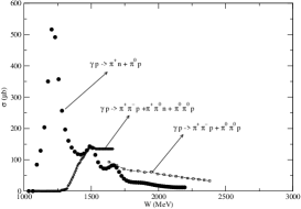
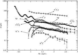
Figure 1: The total cross section data of meson production in $\gamma p$ reaction. Left: $1-\pi$ and $2-\pi$ production are compared. Right: KY ( $K^{+}\Lambda$, $K^{+}\Sigma^{0}$, $K^{0}\Sigma^{+}$), $\eta p$, and $\omega p$ production are compared with some of the $1-\pi$ and $2-\pi$ production

In practice, the dynamical reaction models describe the meson-baryon reaction mechanisms by using phenomenological Lagrangians which are constructed by using the symmetry properties, in particular the Chiral Symmetry, deduced from many-years’ studies of meson-nucleon reactions. Starting from a set of phenomenological Lagrangians for mesons and baryons, one would ideally like to analyze the meson-baryon reaction data completely within the framework of relativistic quantum field theory. The Bethe-Salpeter (BS) equation has been taken historically as the starting point of such an ambitious approach. The complications involved in solving the BS equation in the simplest Ladder approximation have been known for long time. It contains serious singularities arising from the pinching of the integration over the time component. In addition to the two-body unitarity cut, it has a selected set of n-body unitarity cuts, as explained in great detail in Refs. [15, 16]. Thus it is extremely difficult, if not impossible, to apply the approach based on the Bethe-Salpeter equation to study $N^{*}$ states.

Since 1990 the $\pi N$ and $\gamma N$ reactions have been investigated mainly by using either the three-dimensional reductions[17] of the Bethe-Salpeter equation or the unitary transformation methods[4, 18]. These efforts were motivated mainly by the success of the meson-exchange models of $NN$ scattering[19], and have yielded the meson-exchange models developed by Pearce and Jennings[20], National Taiwan University-Argonne National Laboratory (NTU-ANL) collaboration [21, 22], Gross and Surya[23], Sato and Lee[4, 5], Julich Group[24, 25, 26, 27], Fuda and his collaborators[18, 28], and Utretch-Ohio collaboration[29, 30]. The focus of all of these dynamical models was on the analysis of the data in the $\Delta$ (1232) region. In this article, we will only review the model developed in Refs. [4, 5] by using the unitary transformation method. We will also review its extension[6, 7] to study the $\Delta$ (1232) excitation in neutrino-induced $N(\nu,{\it l}\pi)N$ reactions.

The main challenge of developing dynamical reaction models of meson production reactions in the higher mass $N^{*}$ region can be seen in Fig.1. We see that two-pion photo-production cross sections shown in the left-hand-side become larger than the one-pion photo-production as the $\gamma p$ invariant mass exceeds $W\sim 1.4$ GeV. In the right-hand-side, KY ( $K^{+}\Lambda$, $K^{+}\Sigma^{0}$, $K^{0}\Sigma^{+}$), $\eta p$, and $\omega p$ production cross sections are a factor of about 10 weaker than the dominant $\pi^{+}\pi^{-}p$ production. From the unitarity condition, we have for any single meson production process $\gamma N\rightarrow MB$ with $MB=\pi N,\eta N,\omega N,K\Lambda,K\Sigma$

$$i(T_{MB,\gamma N}-T^{*}_{\gamma N,MB}) = \sum_{M^{\prime}B^{\prime}}T^{*}_{M^{\prime}B^{\prime},MB}\rho_{M^{\prime}B^{\prime}}T_{M^{\prime}B^{\prime},\gamma N}$$ (1)

$$+T^{*}_{\pi\pi N,MB}\rho_{\pi\pi N}T_{\pi\pi N,\gamma N}\,,$$

where $\rho_{\alpha}$ denotes an appropriate phase space factor for the channel $\alpha$. The large two-pion production cross sections seen in Fig.1 indicate that the second term in the right-hand-side of Eq.(1) is significant and hence the single meson production reactions above the $\Delta$ region must be influenced strongly by the coupling with the two-pion channels. Similarly, the two-pion production $\gamma N\rightarrow\pi\pi N$ is also influenced by the transition to two-body $MB$ channel

$$i(T_{\pi\pi N,\gamma N}-T^{*}_{\gamma N,\pi\pi N}) = \sum_{M^{\prime}B^{\prime}}T^{*}_{M^{\prime}B^{\prime},\pi\pi N}\rho_{M^{\prime}B^{\prime}}T_{M^{\prime}B^{\prime},\gamma N}$$ (2)

$$+T^{*}_{\pi\pi N,\pi\pi N}\rho_{\pi\pi N}T_{\pi\pi N,\gamma N}\,.$$

Clearly, a sound dynamical reaction model must be able to describe the two pion production and to account for the above unitarity conditions. Such a model has been developed by using the unitary transformation method in Ref.[8] and applied to investigate $\pi N$ elastic scattering[10], $\gamma N\rightarrow\pi N$ reactions[11] $\pi N\rightarrow\eta N$ reactions[12], and $\pi N\rightarrow\pi\pi N$ reactions[13]. In this article, we will also review these results.

This article is organized as follows. In section 2, we explain the unitary transformation method developed in Ref.[31] using a simple model. The constructed model Hamiltonian for investigating $N^{*}$ states is given in section 3. The multi-channel multi-resonance reaction model developed in Refs.[4, 8] for calculating the meson-baryon reaction amplitudes is presented in section 4. In section 5, we give formula for defining the $N$-$N^{*}$ transition form factors and calculating the cross sections of pion production from $\pi N$, $\gamma N$, $N(e,e^{\prime})$, and $N(\nu,{\it l})$ reactions. The results in the $\Delta$ (1232) region and in the higher mass $N^{*}$ region are reviewed in section 6. A summary and discussions of future developments are given in section 7.

2 Unitary Transformation Method

The unitary transformation method was essentially based on the same idea of the Foldy-Wouthuysenth transformation developed in the study of electromagnetic interactions. It was first developed in 1950’s by Fukuda, Sawada and Taketani [32], and independently by Okubo[33]. This approach, called the FST-Okubo method, has been very useful in investigating nuclear electromagnetic currents [34, 35] and relativistic descriptions of nuclear interactions [36, 37, 38]. The advantage of this approach is that the resulting effective Hamiltonian is energy independent and can readily be used in nuclear many-body calculation.

To illustrate the unitary transformation method, we consider the simplest phenomenological Lagrangian density

$${\it L}(x)={\it L}_{0}(x)+{\it L}_{I}(x)\,,$$ (3)

where ${\it L}_{0}(x)$ is the usual free Lagrangians with physical masses $m_{N}$ for the nucleon field $\psi_{N}$ and $m_{\pi}$ for the pion field $\phi_{\pi}$, and

$${\it L}_{I}(x)=\bar{\psi}_{N}(x)\Gamma_{N,\pi N}\psi_{N}(x)\phi_{\pi}(x)\,.$$ (4)

Here $\Gamma_{N,\pi N}$ denotes the physical $\pi NN$ coupling ($\sim f_{\pi NN}$). The Hamiltonian density ${\it H}(x)$ can be derived from Eqs.(3)-(4)by using the standard method of canonical quantization. We then define the Hamiltonian as

$$H=\int{\it H}(\vec{x},t=0)d\vec{x}.$$ (5)

The resulting Hamiltonian can be written as

$$H=H_{0}+H_{I},$$ (6)

with

$$H_{0} = \int d\vec{k}[E_{N}(k)b^{\dagger}_{\vec{k}}b_{\vec{k}}+E_{\pi}(k)a^{\dagger}_{\vec{k}}a_{\vec{k}}],$$ (7)

$$H_{I} = \Gamma_{N\leftrightarrow\pi N}$$ (8)

$$= \int d\vec{k}_{1}d\vec{k}_{2}d\vec{k}\delta(\vec{k}-\vec{k}_{1}-\vec{k}_{2})[(\Gamma_{N,\pi N}(\vec{k}_{1}-\vec{k}_{2})b^{\dagger}_{\vec{k}}b_{\vec{k}_{1}}a_{\vec{k}_{2}})+(h.c)],$$

where $b^{\dagger}$ and $a^{\dagger}$ ($b$ and $a$) are the creation (annihilation) operators for the nucleon and the pion, respectively. For simplicity, we drop the terms involving the anti-nucleon operator. Note that $H$ along with the other constructed generators $\vec{P}$, $\vec{K}$, and $\vec{J}$, as studied in Refs.[36, 37], define the instant-form relativistic quantum mechanical description of $\pi N$ scattering. We will work in the center of mass frame and hence the forms of these other generators of Lorentz group are not relevant in the following derivations.

The essence of the unitary transformation method is to extract an effective Hamiltonian in a ”few-body” space defined by an unitary operator $U$, such that the resulting scattering equations can be solved in practice. Instead of the original equation of motion $H|\alpha>=E_{\alpha}|{\alpha}>$, we consider

$$H^{\prime}|\bar{\alpha}>=E_{\alpha}|\bar{\alpha}>,$$ (9)

where

$$H^{\prime} = UHU^{\dagger}\,,$$ (10)

$$|\bar{\alpha}> = U|\alpha>.$$ (11)

In the approach of Kobayashi, Sato and Ohtsubo[31] (KSO), the first step is to decompose the interaction Hamiltonian $H_{I}$ Eq.(8) into two parts

$$H_{I} = H_{I}^{P}+H_{I}^{Q},$$ (12)

where $H_{I}^{P}$ defines the process $a\rightarrow bc$ with $m_{a}\geq m_{b}+m_{c}$ which can take place in the free space, and $H_{I}^{Q}$ defines the virtual process with $m_{a}<m_{b}+m_{c}$. For the simple interaction Hamiltonian Eq.(8), it is clear that $H^{P}_{I}=0$ and $H^{Q}_{I}=H_{I}$.

The KSO method is to define an appropriate unitary transformation $U$ to eliminate the virtual processes from transformed Hamiltonian $H^{\prime}$. This can be done systematically by using a perturbative expansion of $U$ in powers of coupling constants. As a result the effects of ’virtual processes’ are included in the effective operators in the transformed Hamiltonian.

Defining $U=exp(-iS)$ by a hermitian operator S and expanding $U=1-iS+...$ , the transformed Hamiltonian can be written as

$$H^{\prime} = UHU^{\dagger}$$ (13)

$$= U(H_{0}+H^{P}_{I}+H^{Q}_{I})U^{\dagger}$$

$$= H_{0}+H^{P}_{I}+H^{Q}_{I}+[H_{0},iS\,]+[H_{I},iS\,]+{1\over 2!}\,\Big{[}[H_{0},iS\,],iS\,\Big{]}+\cdots.$$

To eliminate from Eq.(13) the virtual processes which are of first-order in the coupling constant, the KSO method imposes the condition that

$$H^{Q}_{I}+[H_{0},iS\,]=0\,.$$ (14)

Since $H_{0}$ is a diagonal operator in Fock-space , Eq.(14) clearly implies that $iS$ must have the same operator structure of $H^{Q}_{I}$ and is first order in coupling constant. By using Eq.(14), Eq.(13) can be written as

$$H^{\prime}=H_{0}+H_{I}^{\prime}\,,$$ (15)

with

$$H_{I}^{\prime}=H_{I}^{P}+[H_{I}^{P},iS\,]+\frac{1}{2}\,[H_{I}^{Q},iS\,]+\mbox{higher order terms}\,.$$ (16)

Since $H_{I}^{P}$, $H_{I}^{Q}$, and $S$ are all of the first order in the coupling constant, all processes included in the second and third terms of the $H_{I}^{\prime}$ are of the second order in coupling constants.

We now turn to illustrating how the constructed $H_{I}^{\prime}$ of Eq.(16) can be used to describe the $\pi N$ scattering if the higher order terms are dropped. We consider the simple Hamiltonian defined by Eqs.(6)-(8) which gives $H^{P}_{I}=0$ and $H^{Q}_{I}=\Gamma_{N\leftrightarrow\pi N}$. Our first task is to find $S$ by solving Eq.(14) within the Fock space spanned by the eigenstates of $H_{0}$

$$H_{0}|N>=m_{N}|N>\,,$$ (17)

$$H_{0}|\vec{k},\vec{p}>=(E_{\pi}(k)+E_{N}(p))|\vec{k},\vec{p}>\,,$$ (18)

$$H_{0}|\vec{k}_{1},\vec{k}_{2},\vec{p}>=((E_{\pi}(k_{1})+E_{\pi}(k_{2})+E_{N}(p))|\vec{k}_{1},\vec{k}_{2},\vec{p}>\,,$$ (19)

$$\cdot\cdot\cdot\cdot$$

For two eigenstates $f$ and $i$ of $H_{0}$, the solution of Eq.(14) clearly is

$$<f|(iS)|i>=-\frac{<f|H^{Q}_{I}|i>}{E_{f}-E_{i}}\,.$$ (20)

For the considered $H^{Q}_{I}=\Gamma_{N\leftrightarrow\pi N}$ we thus get the following non-vanishing matrix elements

$$<\vec{k},\vec{p}|(iS)|N> = -\Gamma_{N,\pi N}(k)\frac{\delta(\vec{k}+\vec{p})}{E_{\pi}(k)+E_{N}(p)-m_{N}}\,,$$ (21)

$$<N|(iS)|\vec{k}^{\,\prime},\vec{p}^{\,\prime}> = -\frac{\delta(\vec{k}^{\,\prime}+\vec{p}^{\,\prime})}{m_{N}-E_{\pi}(k^{\prime})-E_{N}(p^{\prime})}\Gamma^{*}_{N,\pi N}(\vec{k}^{\,\prime})\,,$$ (22)

and

$$<\vec{k}_{1},\vec{k}_{2},\vec{p}|(iS)|\vec{k}^{\prime},\vec{p}^{\,\prime}> = \frac{-\delta(\vec{k}^{\prime}-\vec{k}_{2})\delta(\vec{p}^{\prime}-\vec{k}_{1}-\vec{p})\Gamma^{*}_{N,\pi N}(k_{1})}{E_{\pi}(k_{1})+E_{\pi}(k_{2})+E_{N}(p)-E_{\pi}(k^{\prime})-E_{N}(p^{\prime})}+(1\leftrightarrow 2)$$ (23)

$$= \Gamma^{*}_{N,\pi N}(k_{1})\frac{-\delta(\vec{k}^{\prime}-\vec{k}_{2})\delta(\vec{p}^{\prime}-\vec{k}_{1}-\vec{p})}{E_{\pi}(k_{1})+E_{N}(p)-E_{N}(p^{\prime})}+(1\leftrightarrow 2)\,,$$

$$<\vec{k},\vec{p}|(iS)|\vec{k}_{1},\vec{k}_{2},\vec{p}> = \frac{-\delta(\vec{k}-\vec{k}_{1})\delta(\vec{p}^{\prime}-\vec{k}_{2}-\vec{p})\Gamma_{N,\pi N}(k_{2})}{E_{\pi}(k)+E_{N}(p)-E_{\pi}(k_{1})-E_{\pi}(k_{2})-E_{N}(p)}+(1\leftrightarrow 2)$$ (24)

$$= \Gamma_{N,\pi N}(k_{2})\frac{-\delta(\vec{k}-\vec{k}_{1})\delta(\vec{p}^{\prime}-\vec{k}_{2}-\vec{p})}{E_{N}(p)-E_{\pi}(k_{2})-E_{N}(p)}+(1\leftrightarrow 2)\,.$$

With the above matrix elements and recalling that $H^{P}_{I}=0$ and $H^{Q}_{I}=\Gamma_{N\leftrightarrow\pi N}$ for the considered simple case, the matrix element of the effective Hamiltonian Eq.(16) in the center of mass frame ($\vec{p}=-\vec{k}$ and $\vec{p}^{\prime}=-\vec{k}^{\prime}$) is

$$<\vec{k}|H_{I}^{\prime}|\vec{k}^{\prime}> = \frac{1}{2}\sum_{I}[(<\vec{k}|\Gamma_{N\leftrightarrow\pi N}|I><I|(iS)|\vec{k}^{\prime}>$$ (25)

$$-<\vec{k}|(iS)|I><I|\Gamma_{N\leftrightarrow\pi N}|\vec{k}^{\prime}>]\,.$$

The only possible intermediate states are $|I>=|N>+|\pi(k_{1})\pi(k_{2})N(P_{I})>$. By using Eqs.(21)-(24) we then obtain

$$<\vec{k}|H_{I}^{\prime}|\vec{k}^{\prime}> = v^{(s)}(\vec{k},\vec{k}^{\prime})+v^{(u)}(\vec{k},\vec{k}^{\prime})\,.$$ (26)

where

$$v^{(s)}(\vec{k},\vec{k}^{\prime}) = \frac{1}{2}\Gamma^{*}_{N,\pi N}(k)[\frac{1}{E_{\pi}(k)+E_{N}(k)-m_{N}}$$ (27)

$$+\frac{1}{E_{\pi}(k^{\prime})+E_{N}(k^{\prime})-m_{N}}]\Gamma^{*}_{N,\pi N}(k^{\prime})\,,$$

$$v^{(u)}(\vec{k},\vec{k}^{\prime}) = \frac{1}{2}\Gamma^{*}_{N,\pi N}(k^{\prime})[\frac{1}{E_{N}(k)-E_{\pi}(k^{\prime})-E_{N}(\vec{k}+\vec{k}^{\prime})}$$ (28)

$$+\frac{1}{E_{N}(k^{\prime})-E_{\pi}(k)-E_{N}(\vec{k}+\vec{k}^{\prime})}]\Gamma_{N,\pi N}(k)\,.$$

Note that up to the same order Eq.(26) should have an additional term which is the one-pion-loop contribution to the single nucleon state. Such a mass renormalization term is dropped in practice, since it is part of the physical nucleon mass in the resulting effective Hamiltonian. If we treat this mass renormalization explicitly, we then will not get a solvable few-body problem, but a many-body problem which is as complicated as the original field theory problem. We also note that $v^{(s)}$ of Eq.(27) is due to the intermediate ”physical” nucleon state state $|I>=|N>$. This is the consequence of the unitary transformation which eliminates the ”virtual” $\pi N\leftrightarrow N$ process. Here we see an important difference between $v^{(s)}$ and the so-called nucleon-pole term from approaches based on some models based on the three-dimensional reduction of Bethe-Salpeter equations and the time-order perturbation theory[27]. There is no bare mass $m^{0}_{N}$ and energy-dependence in $v^{(s)}$.

With the above derivations, the effective Hamiltonian Eq.(16) can be explicitly written as

$$H^{\prime}=H_{0}+V\,,$$ (29)

where

$$H_{0} = \int d\vec{k}[E_{N}(k)b^{\dagger}_{\vec{k}}b_{\vec{k}}+E_{\pi}(k)a^{\dagger}_{\vec{k}}a_{\vec{k}}]\,,$$ (30)

$$V = \int d\vec{k}d\vec{k}^{\prime}[v^{(s)}(\vec{k},\vec{k}^{\prime})+v^{(u)}(\vec{k},\vec{k}^{\prime})]a^{\dagger}_{\vec{k}}b^{\dagger}_{-\vec{k}}a_{\vec{k}^{\prime}}b_{-\vec{k}^{\prime}}\,.$$ (31)

To see the analytic properties of the reaction amplitudes based on the effective Hamiltonian Eq.(29), let us first recall how the bound states and resonances are defined in a Hamiltonian formulation. In operator form the reaction amplitude is defined by

$$t(E)=V+V\frac{1}{E-H_{0}+i\epsilon}t(E)\,,$$ (32)

or

$$t(E)=V+V\frac{1}{E-H^{\prime}+i\epsilon}V\,.$$ (33)

The analytic structure of scattering amplitude can be most transparently seen by using the spectral expansion of the Low equation Eq.(33)

$$<k^{\prime}|t(E)|k> = <k^{\prime}|V|k>+\sum_{i}\frac{<k^{\prime}|V|\Phi_{\epsilon_{i}}><\Phi_{\epsilon_{i}}|V|k>}{E-\epsilon_{i}}$$

$$+\int_{E_{th}}^{\infty}\frac{<k^{\prime}|V|\Psi^{(+)}_{E^{\prime}}><\tilde{\Psi}^{(+)}_{E^{\prime}}|V|k>}{E-E^{\prime}+i\epsilon}\,,$$

where $E_{th}$ is the threshold of the reaction channels, $\Phi_{\epsilon_{i}}$ and $\Psi^{(+)}_{E^{\prime}}$ are the discrete bound states and the scattering states, respectively. They form a complete set and satisfy

$$H^{\prime}|\Phi_{\epsilon_{i}}> = \epsilon|\Phi_{\epsilon_{i}}>\,,$$ (35)

$$H^{\prime}|\Psi^{(+)}_{E^{\prime}}> = E^{\prime}|\Psi^{(+)}_{E^{\prime}}>\,.$$ (36)

Of course bound state energies $\epsilon_{i}$ are below the production threshold $E_{th}$. We now note that because of the two-body nature of $V$ defined by Eq (31), Eq.(35) has the one-nucleon solution $H^{\prime}|N>=H_{0}|N>=m_{N}|N>$. But it does not contribute to the second term of Eq.(LABEL:eq:c1) because $<\pi N|V|N>=0$. Thus the amplitude Eq.(LABEL:eq:c1) does not have a nucleon pole which corresponds to bound state with a mass of physical nucleon and is formed by the $physical$ $N$ and $\pi$ of the starting Lagrangian Eq. (3). This is consistent with the experiment. Clearly, our approach is very different from the S-matrix approach which requires that the $\pi N$ scattering amplitude must have a pole at $E=m_{N}$. Similar feature is also obtained by using the unitary transformation of Shebeko et al.[39, 40].

To end this section, we mention that the unitarity condition only requires that an acceptable model must have unitarity cut in physical region $E\geq m_{\pi}+m_{N}$. This is trivially satisfied in the the model defined by the effective Hamiltonian Eqs.(30)-(31) since the interaction $V$ is energy independent. This is an important advantage in applying the method of unitary transformation to develop a multi-channels multi-resonances reaction models for investigating meson-nucleon reactions in the nucleon resonance region, as developed in Ref.[8]. In a model with an energy-dependent $V$ such as the Julich model[27] the unitarity condition is much more difficult to satisfy, and the analytic continuation of the scattering t-matrix defined by Eqs.(LABEL:eq:c1) to complex $E$-plane is in general much more complex.

3 Model Hamiltonian

With the unitary transformation method explained in section 2, it is straightforward to derive a model Hamiltonian for constructing a coupled-channel reaction model with $\gamma N$, $\pi N$, $\eta N$ and $\pi\pi N$ channels. Since significant parts of the $\pi\pi N$ production are known experimentally to be through the unstable states $\pi\Delta$, $\rho N$, and perhaps also $\sigma N$, we will also include $bare$ $\Delta$, $\rho$ and $\sigma$ degrees of freedom in our formulation. Furthermore, we introduce $bare$ $N^{*}$ states to represent the quark-core components of the nucleon resonances. The model is expected to be valid up to $W=2$ GeV below which three pion production is very weak.

The starting point is a set of Lagrangians describing the interactions between mesons ($M=\gamma,\pi,\eta,\rho,\omega,\sigma\cdot\cdot\cdot$) and baryons ($B=N,\Delta,N^{*}\cdot\cdot\cdot$). These Lagrangian are constrained by various well-established symmetry properties, such as the invariance under isospin, parity, and gauge transformation. The chiral symmetry is also implemented as much as we can. The considered Lagrangians are given in Ref.[8]. For completeness, we recall in Appendix A parts of these Lagrangians which were used in investigating the $\Delta$ (1232) resonance.

By applying the standard canonical quantization, we obtain a Hamiltonian of the following form

$$H = \int{\it h(\vec{x},t=0)}d\vec{x}$$ (37)

$$= H_{0}+H_{I}\,,$$

where ${\it h(\vec{x},t)}$ is the Hamiltonian density constructed from the starting Lagrangians and the conjugate momentum field operators. In Eq.(37), $H_{0}$ is the free Hamiltonian and

$$H_{I}=\sum_{M,B,B^{\prime}}\Gamma_{MB\leftrightarrow B^{\prime}}+\sum_{M,M^{\prime},M^{\prime\prime}}h_{M^{\prime}M^{\prime\prime}\leftrightarrow M}\,,$$ (38)

where $\Gamma_{MB\leftrightarrow B^{\prime}}$ describes the absorption and emission of a meson($M$) by a baryon($B$) such as $\pi N\leftrightarrow N$ and $\pi N\leftrightarrow\Delta$, and $h_{M^{\prime}M^{\prime\prime}\leftrightarrow M}$ describes the vertex interactions between mesons such as $\pi\pi\leftrightarrow\rho$ and $\gamma\pi\leftrightarrow\pi$.

Figure 2: Basic mechanisms of the Model Hamiltonian defined in Eqs.(42)-(44).

Our main step is to derive from Eqs.(37)-(38) an effective Hamiltonian which contains interactions involving $\pi\pi N$ three-particle states. This is accomplished by applying the unitary transformation method up to the third order in interaction $H_{I}$ of Eq.(38). The resulting effective Hamiltonian is of the following form

$$H_{eff}=H_{0}+V\,,$$ (39)

with

$$H_{0}=\sum_{\alpha}K_{\alpha}\,,$$ (40)

where $K_{\alpha}=\sqrt{m_{\alpha}^{2}+\vec{p_{\alpha}}^{2}}$ is the free energy operator of particle $\alpha$ with a mass $m_{\alpha}$, and the interaction Hamiltonian is

$$V=\Gamma_{V}+v_{22}+v^{\prime}\,,$$ (41)

where

$$\Gamma_{V} = \{\sum_{N^{*}}(\sum_{MB}\Gamma_{N^{*}\rightarrow MB}+\Gamma_{N^{*}\rightarrow\pi\pi N})+\sum_{M^{*}}h_{M^{*}\rightarrow\pi\pi}\}+\{h.c.\}\,,$$ (42)

$$v_{22} = \sum_{MB,M^{\prime}B^{\prime}}v_{M^{\prime}B^{\prime},MB}+v_{\pi\pi}\,.$$ (43)

Here ${h.c.}$ denotes the hermite conjugate of the terms on its left-hand-side. In the above equations, $MB=\gamma N,\pi N,\eta N,\pi\Delta,\rho N,\sigma N$ represent the considered meson-baryon states. The resonance associated with the $bare$ baryon state $N^{*}$ is induced by the vertex interactions $\Gamma_{N^{*}\rightarrow MB}$ and $\Gamma_{N^{*}\rightarrow\pi\pi N}$. Similarly, the $bare$ meson states $M^{*}$ = $\rho$, $\sigma$ can develop into resonances through the vertex interaction $h_{M^{*}\rightarrow\pi\pi}$. These vertex interactions are illustrated in Fig.2(a). Note that the masses $M^{0}_{N^{*}}$ and $m^{0}_{M^{*}}$ of the bare states $N^{*}$ and $M^{*}$ are the parameters of the model which will be determined by fitting the $\pi N$ and $\pi\pi$ scattering data. They differ from the empirically determined resonance positions by mass shifts which are due to the coupling of the bare states with the meson-baryon $scattering$ states. It is thus reasonable to speculate that these bare masses can be identified with the mass spectrum predicted by the hadron structure calculations which do not account for the meson-baryon $continuum$ scattering states, such as the calculations based on the constituent quark models which do not have meson-exchange quark-quark interactions. It is however much more difficult, but more interesting, to relate these bare masses to the $current$ Lattice QCD calculations which can not account for the scattering states rigorously mainly because of the limitation of the lattice spacing.

In Eq.(43), $v_{M^{\prime}B^{\prime},MB}$ is the non-resonant meson-baryon interaction and $v_{\pi\pi}$ is the non-resonant $\pi\pi$ interaction. They are illustrated in Fig.2(b). The third term in Eq.(41) describes the non-resonant interactions involving $\pi\pi N$ states

$$v^{\prime}=v_{23}+v_{33}\,,$$ (44)

with

$$v_{23} = \sum_{MB}[(v_{\pi\pi N,MB})+(h.c.)]\,,$$

$$v_{33} = v_{\pi\pi N,\pi\pi N}\,.$$

They are illustrated in Fig.2(c). All of these interactions are defined by the tree-diagrams generated from the considered Lagrangians. They are illustrated in Fig.3 for two-body interactions $v_{M^{\prime}B^{\prime},MB}$ and in Fig.4 for $v_{\pi\pi N,MB}$. In practice, we neglect $v_{\pi\pi}$ and $v_{\pi\pi N,\pi\pi N}$. We also only consider $v_{\pi\pi N,\pi N}$ and $v_{\pi\pi N,\gamma N}$ of $v_{\pi\pi N,MB}$. These two interactions are illustrated in Fig.4. The calculations of the matrix elements of these interactions were explained in details in Ref. [8]. Here we only mention that the matrix elements of these interactions are calculated from the usual Feynman amplitudes with the energies of off-mass-shell particles in the intermediate states defined by the three momenta of the initial and final states, as specified by the unitary transformation methods. Thus they are independent of the collision energy $E$.

Figure 3: Mechanisms for $v_{M^{\prime}B^{\prime},MB}$ of Eq. (43): (a) direct s-channel, (b) crossed u-channel, (c) one-particle-exchange t-channel, (d) contact interactions.

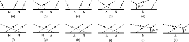
Figure 4: The considered $v_{\pi N,\pi\pi N}$ of $v_{23}$ of Eq.(44).

4 Multi-channels Multi-resonances Reaction Model

Our next task is to derive a set of dynamical coupled-channel equations for describing $\gamma N,\pi N\rightarrow MB$ reactions within the model space $N^{*}\oplus MB\oplus\pi\pi N$. The starting point is the Lippman-Schwinger equation for the scattering T-matrix

$$<a|T(E)|b>=<a|V|b>+<a|V\frac{1}{E-H_{0}+i\epsilon}T(E)|b>\,,$$ (45)

where the interaction $V$ is defined from the effective Hamiltonian in Eqs.(39)-(44). We choose the normalization that the T-matrix is related to the S-matrix by

$$<a|S(E)|b>=\delta_{ab}-2\pi i\delta^{4}(P_{a}-P_{b})<a|T(E)|b>\,.$$ (46)

Since the interaction $V$, defined by Eqs.(41)-(44), is energy independent, it is rather straightforward to follow the formal scattering theory given in Ref.[41] to show that Eq.(45) leads to the following unitarity condition

$$<a|T(E)-T^{\dagger}(E)|b>=-2\pi i\sum_{c}<a|T^{\dagger}(E)|c>\delta(E_{c}-E)<c|T(E)|b>\,,$$ (47)

where $a,b,c$ are the reaction channels in the considered energy region.

We cast Eq. (45) into a more convenient form for practical calculations. In the derivations, the unitarity condition Eq.(47) must be maintained exactly. We achieve this rather complex task by applying the standard projection operator techniques[42], similar to that employed in a study of $\pi NN$ scattering[43]. The details of our derivations are given in Appendix B of Ref. [8]. To explain our coupled-channel equations, it is sufficient to present the formula obtained from setting $\Gamma_{N^{*}\rightarrow\pi\pi N}=0$ in our derivations. Here we explain these equations and discuss their dynamical content.

The resulting $MB\rightarrow M^{\prime}B^{\prime}$ amplitude $T_{M^{\prime}B^{\prime},MB}$ in each partial wave consists of a non-resonant amplitude $t_{M^{\prime}B^{\prime},MB}(E)$ and a resonant amplitude $t^{R}_{M^{\prime}B^{\prime},MB}(E)$ as illustrated in Figs. 5 and 6. It can be written as

$$T_{M^{\prime}B^{\prime},MB}(E) = t_{M^{\prime}B^{\prime},MB}(E)+t^{R}_{M^{\prime}B^{\prime},MB}(E)\,.$$ (48)

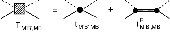
Figure 5: Graphical representations of Eq. (48).

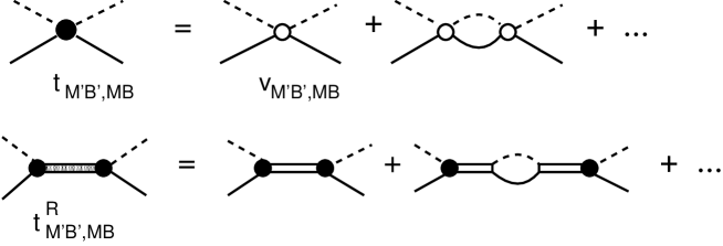
Figure 6: Graphical representations of Eqs. (49) and (57).

Figure 7: Graphical representations of Eqs. (52)-(53).

The second resonant term in the right-hand-side of Eq.(48) is defined by

$$t^{R}_{M^{\prime}B^{\prime},MB}(E)=\sum_{N^{*}_{i},N^{*}_{j}}\bar{\Gamma}_{N^{*}_{i}\rightarrow M^{\prime}B^{\prime}}(E)[D(E)]_{i,j}\bar{\Gamma}_{MB\rightarrow N^{*}_{j}}(E)\,,$$ (49)

with

$$[D(E)^{-1}]_{i,j}(E)=(E-M^{0}_{N^{*}_{i}})\delta_{i,j}-\bar{\Sigma}_{i,j}(E)\,,$$ (50)

where $M_{N^{*}}^{0}$ is the mass of a bare $N^{*}$ state, and the self-energies are

$$\bar{\Sigma}_{i,j}(E)=\sum_{MB}\bar{\Gamma}_{MB\rightarrow N^{*}_{i}}(E)G_{MB}(E)\Gamma_{N^{*}_{j}\rightarrow MB}\,.$$ (51)

In general, the bare states mix with each other through the off-diagonal matrix elements of the self-energies. The dressed vertex interactions in Eq. (49) and Eq. (51) illustrated in Fig. 7 are (defining $\Gamma_{MB\rightarrow N^{*}}=\Gamma^{\dagger}_{N^{*}\rightarrow MB}$)

$$\bar{\Gamma}_{MB\rightarrow N^{*}}(E)={\Gamma_{MB\rightarrow N^{*}}}+\sum_{M^{\prime}B^{\prime}}\Gamma_{M^{\prime}B^{\prime}\rightarrow N^{*}}G_{M^{\prime}B^{\prime}}(E)t_{M^{\prime}B^{\prime},MB}(E)\,,$$ (52)

$$\bar{\Gamma}_{N^{*}\rightarrow MB}(E)=\Gamma_{N^{*}\rightarrow MB}+\sum_{M^{\prime}B^{\prime}}t_{MB,M^{\prime}B^{\prime}}(E)G_{M^{\prime}B^{\prime}}(E)\Gamma_{N^{*}\rightarrow M^{\prime}B^{\prime}}\,.$$ (53)

The meson-baryon propagator $G_{MB}$ in the above equations takes the following form

$$G_{MB}(E)=\frac{1}{E-K_{B}-K_{M}-\Sigma_{MB}(E)+i\epsilon}\,,$$ (54)

where the mass shift $\Sigma_{MB}(E)$ depends on the considered $MB$ channel. It is $\Sigma_{MB}(E)=0$ for the stable particle channels $MB=\pi N,\eta N$. For channels containing an unstable particle, such as $MB=\pi\Delta,\rho N,\sigma N$, we have

$$\Sigma_{MB}(E)=[<MB|g_{V}\frac{P_{\pi\pi N}}{E-K_{\pi}-K_{\pi}-K_{N}+i\epsilon}g^{\dagger}_{V}|MB>]_{un-connected}\,,$$ (55)

with

$$g_{V}=\Gamma_{\Delta\rightarrow\pi N}+h_{\rho\rightarrow\pi\pi}+h_{\sigma\rightarrow\pi\pi}\,.$$ (56)

In Eq.(55) ”$un-connected$” means that the stable particle, $\pi$ or $N$, of the $MB$ state is a spectator in the $\pi\pi N$ propagation. Thus $\Sigma_{MB}(E)$ is just the mass renormalization of the unstable particle in the $MB$ state. It is important to note that the resonant amplitude $t^{R}_{M^{\prime}B^{\prime},MB}(E)$ is influenced by the non-resonant amplitude $t_{M^{\prime}B^{\prime},MB}(E)$, as seen in Eqs. (49)-(53).

The non-resonant amplitudes $t_{M^{\prime}B^{\prime},MB}$ in Eq.(48) and Eqs.(52)-(53) are defined by the following coupled-channel equations

$$t_{M^{\prime},B^{\prime},MB}(E)=V_{M^{\prime}B^{\prime},MB}(E)+\sum_{M^{\prime\prime}B^{\prime\prime}}V_{M^{\prime}B^{\prime},M^{\prime\prime}B^{\prime\prime}}(E)G_{M^{\prime\prime}B^{\prime\prime}}(E)t_{M^{\prime\prime}B^{\prime\prime},MB}(E)\,,$$ (57)

with

$$V_{M^{\prime}B^{\prime},MB}(E)=v_{M^{\prime}B^{\prime},MB}+Z_{{M}^{\prime}{B}^{\prime},MB}(E)\,.$$ (58)

Here $Z_{{M}^{\prime}{B}^{\prime},MB}(E)$ contains the effects due to the coupling with $\pi\pi N$ states. It has the following form

$$Z_{{M}^{\prime}{B}^{\prime},MB}(E) = [<{M}^{\prime}{B}^{\prime}\mid F\frac{P_{\pi\pi N}}{E-H_{0}-\hat{v}_{\pi\pi N}+i\epsilon}F^{\dagger}\mid{M}{B}>]_{connected}\,,$$ (59)

with

$$\hat{v}_{\pi\pi N} = v_{\pi N,\pi N}+v_{\pi\pi}+v_{\pi\pi N,\pi\pi N}\,,$$ (60)

$$F = g_{V}+v_{MB,\pi\pi N}\,,$$ (61)

where $g_{V}$ has been defined in Eq.(56). Note that the dis-connected term in Eq.(59) is already included in the mass shifts $\Sigma_{MB}$ of the propagator Eq.(54) and must be removed to avoid double counting.

The appearance of the projection operator $P_{\pi\pi N}$ in Eqs.(55) and (59) is the consequence of the unitarity condition Eq.(47). To isolate the effects entirely due to the vertex interaction $g_{V}=\Gamma_{\Delta\rightarrow\pi N}+h_{\rho\rightarrow\pi\pi}+h_{\sigma\rightarrow\pi\pi}$, we use the operator relation

$$\frac{1}{E-H_{0}-v}=\frac{1}{E-H_{0}}+\frac{1}{E-H_{0}}v\frac{1}{E-H_{0}-v}$$ (62)

to decompose the $\pi\pi N$ propagator of Eq.(59) to write

$$Z_{M^{\prime}B^{\prime},MB}(E)=Z^{(E)}_{M^{\prime}B^{\prime},MB}(E)+Z^{(I)}_{M^{\prime}B^{\prime},MB}(E)\,.$$ (63)

The first term is

$$Z^{(E)}_{M^{\prime}B^{\prime},MB}(E) = [<M^{\prime}B^{\prime}\mid g_{V}\frac{P_{\pi\pi N}}{E-H_{0}+i\epsilon}g^{\dagger}_{V}\mid MB>]_{connected}\,.$$ (64)

Obviously, $Z^{(E)}_{M^{\prime}B^{\prime},MB}(E)$ is the one-particle-exchange interaction between unstable particle channels $\pi\Delta$, $\rho N$, and $\sigma N$, as illustrated in Fig.8. The second term of Eq.(63) is

$$Z^{(I)}_{M^{\prime}B^{\prime},MB}(E)=<M^{\prime}B^{\prime}\mid F\frac{P_{\pi\pi N}}{E-H_{0}+i\epsilon}t_{\pi\pi N,\pi\pi N}(E)\frac{P_{\pi\pi N}}{E-H_{0}+i\epsilon}F^{\dagger}\mid MB>$$

$$+<M^{\prime}B^{\prime}\mid g_{V}\frac{P_{\pi\pi N}}{E-H_{0}+i\epsilon}v^{\dagger}_{\pi\pi N,MB}\mid MB>$$

$$+<M^{\prime}B^{\prime}\mid v_{M^{\prime}B^{\prime},\pi\pi N}\frac{P_{\pi\pi N}}{E-H_{0}+i\epsilon}g^{\dagger}_{V}\mid MB>$$

$$+<M^{\prime}B^{\prime}\mid v_{M^{\prime}B^{\prime},\pi\pi N}\frac{P_{\pi\pi N}}{E-H_{0}+i\epsilon}v^{\dagger}_{\pi\pi N,MB}\mid MB>\,.$$ (65)

Here $t_{\pi\pi N,\pi\pi N}(E)$ is a three-body scattering amplitude defined by

$$t_{\pi\pi N,\pi\pi N}(E)=\hat{v}_{\pi\pi N}+\hat{v}_{\pi\pi N}\frac{1}{E-K_{\pi}-K_{\pi}-K_{N}-\hat{v}_{\pi\pi N}+i\epsilon}\hat{v}_{\pi\pi N}\,,$$ (66)

where $\hat{v}_{\pi\pi N}$ has been defined in Eq.(60).

Figure 8: One-particle-exchange interactions $Z^{(E)}_{\pi\Delta,\pi\Delta}(E)$, $Z^{(E)}_{\pi\Delta,\rho N}$ and $Z^{(E)}_{\pi\Delta,\sigma N}$ of Eq. (64).

The amplitudes $T_{M^{\prime}B^{\prime},MB}=t_{M^{\prime}B^{\prime},MB}+t^{R}_{M^{\prime}B^{\prime},MB}$ defined by Eq.(48) can be used directly to calculate the cross sections of $\pi N\rightarrow\pi N,\eta N$ and $\gamma N\rightarrow\pi N,\eta N$ reactions. They are also the input to the calculations of the two-pion production amplitudes. The two-pion production amplitudes resulted from our derivations are illustrated in Fig.9. They can be cast exactly into the following form

$$T_{\pi\pi N,MB}(E)=T^{dir}_{\pi\pi N,MB}(E)+T^{\pi\Delta}_{\pi\pi N,MB}(E)+T^{\rho N}_{\pi\pi N,MB}(E)+T^{\sigma N}_{\pi\pi N,MB}(E)\,,$$ (67)

with

$$T^{dir}_{\pi\pi N,MB}(E)=<\psi^{(-)}_{\pi\pi N}(E)|\sum_{M^{\prime}B^{\prime}}v_{\pi\pi N,M^{\prime}B^{\prime}}[\delta_{M^{\prime}B^{\prime},MB}$$

$$+G_{M^{\prime}B^{\prime}}(E)(t_{M^{\prime}B^{\prime},MB}(E)+t^{R}_{M^{\prime}B^{\prime},MB})]|MB>\,,$$ (68)

$$T^{\pi\Delta}_{\pi\pi N,MB}(E)=<\psi^{(-)}_{\pi\pi N}(E)|\Gamma^{\dagger}_{\Delta\rightarrow\pi N}G_{\pi\Delta}(E)[t_{\pi\Delta,MB}(E)+t^{R}_{\pi\Delta,MB}(E)]|MB>\,,$$ (69)

$$T^{\rho N}_{\pi\pi N,MB}(E)=<\psi^{(-)}_{\pi\pi N}(E)|h^{\dagger}_{\rho\rightarrow\pi\pi}G_{\rho N}(E)[t_{\rho N,MB}(E)+t^{R}_{\rho N,MB}(E)]|MB>\,,$$ (70)

$$T^{\sigma N}_{\pi\pi N,MB}(E)=<\psi^{(-)}_{\pi\pi N}(E)|h^{\dagger}_{\sigma\rightarrow\pi\pi}G_{\sigma N}(E)[t_{\sigma N,MB}(E)+t^{R}_{\sigma N,MB}(E)]|MB>\,.$$ (71)

In the above equations, the $\pi\pi N$ scattering wave function is defined by

$$<\psi^{(-)}_{\pi\pi N}(E)| = <\pi\pi N|\Omega^{(-)\dagger}_{\pi\pi N}(E)\,,$$ (72)

where the scattering operator is defined by

$$\Omega^{(-)\dagger}_{\pi\pi N}(E)=<\pi\pi N|[1+t_{\pi\pi N,\pi\pi N}(E)\frac{1}{E-K_{\pi}-K_{\pi}-K_{N}+i\epsilon}]\,.$$ (73)

Here the three-body scattering amplitude $t_{\pi\pi N,\pi\pi N}(E)$ is determined by the non-resonant interactions $v_{\pi\pi}$, $v_{\pi N,\pi N}$ and $v_{\pi\pi N,\pi\pi N}$, as defined by Eq.(66).

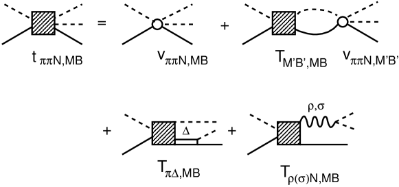
Figure 9: Graphical representations of $T_{\pi\pi N,MB}$ defined by Eqs. (67)-(73).

We note here that the direct production amplitude $T^{dir}_{\pi\pi N,MB}(E)$ of Eq.(68) is due to $v_{\pi\pi N,MB}$ interaction, while the other three terms are through the unstable $\pi\Delta$, $\rho N$, and $\sigma N$ states illustrated in Fig.9. Each term has the contributions from the non-resonant amplitude $t_{M^{\prime}B^{\prime},MB}(E)$ and resonant term $t^{R}_{M^{\prime}B^{\prime},MB}(E)$.

5 Cross Sections and $N$-$N^{*}$ Transition Form Factors

In this section, we give formula for calculating the cross sections of all electroweak pion production reactions. Their relations with the commonly used CGLN and mutipole amplitudes are given in appendix B. For later discussions in section 5, we also present formula for calculating the electromagnetic $N$-$N^{*}$ transition form factors which are the main focus of recent studies of electromagnetic meson production reactions.

5.1 Cross Section Formula

With the relation Eq.(46) between the S- and T- matrices and the normalization $<\vec{k}|\vec{k}^{\,{}^{\prime}}>=\delta(\vec{k}-\vec{k}^{\,{}^{\prime}})$, the amplitude $T_{\gamma N,\pi N}$ for the pion photoproduction reaction $\gamma(\vec{q})+N(-\vec{q})\rightarrow\pi(\vec{k})+N(-\vec{k})$ defined by Eq. (48) can be written in the final $\pi N$ center of mass frame as (suppressing spin-isospin indices)

$$T_{\pi N,\gamma N} = \frac{1}{(2\pi)^{3}}\frac{m_{N}}{\sqrt{E_{N}(q)E_{N}(k)2E_{\pi}(k)2q}}[eJ_{em}\cdot\epsilon_{\gamma}].$$ (74)

Here $\epsilon_{\gamma}$ is the polarization vector of photon. In the tree-diagram approximation, the current matrix element $J_{em}$ is of the form of $[\bar{u}_{-\vec{p}}\,I\,u_{-\vec{q}}]$, where $I$ is the usual invariant amplitudes calculated from the Lagrangian $L(x)=j^{\mu}_{em}(x)A_{\mu}(x)$, where $j^{\mu}_{em}(x)$ is the electromagnetic current operator and $A_{\mu}(x)$ is the electromagnetic field. Similarly the amplitudes for the electroweak pion production reactions $e(p_{e})+N(p)\rightarrow e^{\prime}(p_{e^{\prime}})+\pi(k)+N(p^{\prime})$, $\nu_{e}(p_{\nu})+N(p)\rightarrow e^{-}(p_{e^{\prime}})+\pi(k)+N(p^{\prime})$, and $\nu(p_{\nu})+N(p)\rightarrow\nu(p_{\nu^{\prime}})+\pi(k)+N(p^{\prime})$ can be written as

$$T_{e^{\prime}\pi N,eN} = \frac{1}{(2\pi)^{9/2}}\frac{m_{N}}{\sqrt{E_{N}(p)E_{N}(p^{\prime})2E_{\pi}(k)}}\frac{e^{2}}{q^{2}}J_{em}\cdot L_{em},$$ (75)

$$T_{e^{\prime}\pi N,\nu_{e}N} = \frac{1}{(2\pi)^{9/2}}\frac{m_{N}}{\sqrt{E_{N}(p)E_{N}(p^{\prime})2E_{\pi}(k)}}\frac{G_{F}\cos\theta_{c}}{\sqrt{2}}J_{cc}\cdot L_{cc},$$ (76)

$$T_{\nu^{\prime}\pi N,\nu N} = \frac{1}{(2\pi)^{9/2}}\frac{m_{N}}{\sqrt{E_{N}(p)E_{N}(p^{\prime})2E_{\pi}(k)}}\frac{G_{F}}{\sqrt{2}}J_{nc}\cdot L_{nc},$$ (77)

where $J^{\mu}_{cc}$, $J^{\mu}_{nc}$ are the matrix elements of charged current and neutral current, respectively. The lepton current matrix elements are

$$L^{\mu}_{em} = \bar{u}(p_{e^{\prime}})\gamma^{\mu}u(p_{e}),$$ (78)

$$L^{\mu}_{cc} = \bar{u}(p_{e^{\prime}})\gamma^{\mu}(1-\gamma_{5})u(p_{\nu}),$$ (79)

$$L^{\mu}_{nc} = \bar{u}(p_{\nu^{\prime}})\gamma^{\mu}(1-\gamma_{5})u(p_{\nu}).$$ (80)

The pion production current, $J^{\mu}_{\alpha}$($\alpha=em,cc,nc$) can be written in terms of commonly used CGLN amplitudes and multipole amplitudes. These are summarized in appendix B.

The differential cross sections of pion productions reactions due to electromagnetic ($em$) and charged weak current ($cc$) in the massless leptons ($m_{e}=0$) limit can be written as

$$\frac{d\sigma_{em}^{5}}{dE_{e^{\prime}}d\Omega_{e^{\prime}}d\Omega_{\pi}^{*}}=\frac{1}{4}\frac{e^{4}}{Q^{4}}\frac{E_{e^{\prime}}}{E_{e}}\frac{Q^{2}}{1-\epsilon}\frac{Ek_{\pi}}{2\pi^{3}m_{N}}(\frac{m_{N}}{4\pi E})^{2}R_{em},$$ (81)

$$\frac{d\sigma_{cc}^{5}}{dE_{e^{\prime}}d\Omega_{e^{\prime}}d\Omega_{\pi}^{*}}=\frac{G_{F}^{2}\cos^{2}\theta_{c}}{2}\frac{E_{e^{\prime}}}{E_{\nu}}\frac{Q^{2}}{1-\epsilon}\frac{Ek_{\pi}}{2\pi^{3}m_{N}}(\frac{m_{N}}{4\pi E})^{2}R_{cc}.$$ (82)

where $E$ is the invariant mass of the final $\pi N$ state, $\epsilon$ is defined by the lepton scattering angle $\theta_{lep}$ as $\epsilon=1/[1+2\frac{|\bm{q}_{L}|^{2}}{Q^{2}}\tan^{2}\frac{\theta_{lep}}{2}]$ and $k_{\pi}$ is pion momentum in the $\pi N$ center of mass system. The functions $R_{\alpha}$ depends on the pion angle with respect to the direction of momentum transfer $\vec{q}$ and also the angle $\phi_{\pi}$ between the the $\pi-N$ plane and the plane of the incoming and outgoing leptons. Explicitly, we have

$$R_{em} = R_{em}^{T}+\epsilon R_{em}^{L}+\sqrt{2\epsilon(1+\epsilon)}R^{LT}_{em,c}\cos\phi_{\pi}+\epsilon R^{TT}_{em,c}\cos 2\phi_{\pi}],$$ (83)

$$R_{cc} = R_{cc}^{T}+\epsilon R_{cc}^{L}+\sqrt{2\epsilon(1+\epsilon)}(R_{cc,c}^{LT}\cos\phi_{\pi}+R_{cc,s}^{LT}\sin\phi_{\pi})$$ (84)

$$+\epsilon(R_{cc,c}^{TT}\cos 2\phi_{\pi}+R_{cc,s}^{TT}\sin 2\phi_{\pi})\,.$$

The structure functions $R^{\beta}_{\alpha}$ in the above equations are calculated from the current $J^{\mu}_{\alpha}$ for the $N+j_{\alpha}\rightarrow\pi+N$ introduced in Eqs. (74)-(77) in the pion-nucleon center of mass system. It is common to choose the momentum transfer of leptons as the quantization z-direction $\vec{q}=|\vec{q}\ |(0,0,1)$ and set the outgoing pion on the x-z plane $\vec{k}_{\pi}=|\vec{k}_{\pi}|(\sin\theta,0,\cos\theta)$. The structure functions can then be written as

$$R_{\alpha}^{T} = \sum[\frac{|J_{\alpha}^{x}|^{2}+|J_{\alpha}^{y}|^{2}}{2}-\sqrt{1-\epsilon^{2}}\mbox{Im}(J_{\alpha}^{x}J_{\alpha}^{y*})]\,,$$ (85)

$$R_{\alpha}^{L} = \sum\frac{Q^{2}}{|\bm{q}_{c}|^{2}}|\bar{J}_{\alpha}^{0}|^{2}\,,$$ (86)

$$R^{LT}_{\alpha,c} = \sum\sqrt{\frac{Q^{2}}{|\bm{q}_{c}|^{2}}}{}[-\mbox{Re}(\bar{J}_{\alpha}^{0}J_{\alpha}^{x*})+\sqrt{\frac{1-\epsilon}{1+\epsilon}}\mbox{Im}(\bar{J}_{\alpha}^{0}J_{\alpha}^{y*})]\,,$$ (87)

$$R^{LT}_{\alpha,s} = \sum\sqrt{\frac{Q^{2}}{|\bm{q}_{c}|^{2}}}{}[\mbox{Re}(\bar{J}_{\alpha}^{0}J_{\alpha}^{y*})+\sqrt{\frac{1-\epsilon}{1+\epsilon}}\mbox{Im}(\bar{J}_{\alpha}^{0}J_{\alpha}^{x*})]\,,$$ (88)

$$R^{TT}_{\alpha,c} = \sum\frac{|J_{\alpha}^{x}|^{2}-|J_{\alpha}^{y}|^{2}}{2}\,,$$ (89)

$$R^{TT}_{\alpha,s} = -\sum\mbox{Re}(J_{\alpha}^{x}J_{\alpha}^{y*})\,,$$ (90)

where $\alpha=em,cc$, and we have defined

$$\bar{J}_{\alpha}^{0} = J_{\alpha}^{0}+\omega q\cdot J_{\alpha}/Q^{2}\,.$$ (92)

The spin sum of the nucleons $\sum$ is

$$\sum=\frac{1}{2}\sum_{s_{N},s_{N}^{\prime}}\,.$$ (93)

For investigating the weak pion production reactions induced by $\mu$ neutrinos, the above formula need to be modified to include the finite mass $m_{\mu}$ of the outgoing $\mu$ lepton. These formula were given in Ref. [6] and were used in obtaining the results to be reviewed in section 6.2. The cross section formula for the neutral current reactions can be obtained by replacing $G_{F}\cos\theta_{c}$ and $J_{cc}$ of Eq. (82) with $G_{F}$ and $J_{nc}$.

For the structure functions of the electromagnetic current $R_{em}$, we use $\bar{J}^{0}=J^{0}$ and $\mbox{Im}(J_{em}^{x}J_{em}^{y,*})=\mbox{Im}(J_{em}^{0}J_{em}^{y,*})=0$. For pion electroproduction cross sections, it is convenient to write Eqs.(81) as

$$\frac{d\sigma_{em}^{5}}{dE_{e^{\prime}}d\Omega_{e^{\prime}}d\Omega_{\pi}^{*}} = \Gamma_{T}\frac{d\sigma^{v}}{d\Omega^{*}_{\pi}}\,,$$ (94)

with

$$\Gamma_{T} = \frac{\alpha}{2\pi^{2}Q^{2}}\frac{E_{e^{\prime}}}{E_{e}}\frac{q_{\gamma,L}}{1-\epsilon}\,,$$ (95)

$$\frac{d\sigma^{v}}{d\Omega^{*}_{\pi}} = \frac{k_{\pi}}{q_{\gamma}}(\frac{m_{N}}{4\pi E})^{2}e^{2}R_{em}\,,$$ (96)

where $q_{\gamma}=(E^{2}-m_{N}^{2})/(2E)$ and $q_{\gamma,L}=(E^{2}-m_{N}^{2})/(2m_{N})$.

5.2 $N^{*}$ Transition Form Factor

The main objective of analyzing the data of electromagnetic meson production reactions is to extract the $\gamma N\rightarrow\bar{N}^{*}(JT)$ transition form factors with $J$ and $T$ denoting the spin and isospin of a nucleon resonance. In this section, we define these quantities within our formulation.

Our starting point is the following Lagrangian density within the framework of the relativistic quantum field theory

$$L_{em}(x)=ej^{\mu}_{em}(x)A_{\mu}(x)\,,$$

where $A_{\mu}(x)$ is the electromagnetic field and $j_{em}^{\mu}(x)$ is the current operator. In the rest frame of $\bar{N}^{*}$, the electromagnetic $\gamma N(s_{z},t_{z})\rightarrow\bar{N}^{*}(JT)$ transition form factors are usually characterized[44, 45] by the helicity amplitudes $A_{\lambda}$ for the spatial components and $S_{1/2}$ for the time component of currents :

$$A^{JT}_{3/2,t_{z}}(Q^{2}) = X<\bar{N}^{*}(JT)|\vec{j}_{em}(Q^{2})\cdot\vec{\epsilon}_{1}|N(s_{z}=1/2,t_{z})>\,,$$ (97)

$$A^{JT}_{1/2,t_{z}}(Q^{2}) = X<\bar{N}^{*}(JT)|\vec{j}_{em}(Q^{2})\cdot\vec{\epsilon}_{1}|N(s_{z}=-1/2,t_{z})>\,,$$ (98)

$$S^{JT}_{1/2,t_{z}}(Q^{2}) = X<\bar{N}^{*}(JT)|j^{0}_{em}(Q^{2})|N(s_{z}=1/2,t_{z})>\,,$$ (99)

where $Q^{2}=-q^{2}=\vec{q}^{\,2}-\omega^{2}$ is defined by the photon momentum $q^{\mu}=(\omega,\vec{q})$, and

$$X=\frac{e}{\sqrt{2K_{\gamma}}},$$ (100)

$$\vec{\epsilon}_{1}=\frac{\vec{e}_{x}+i\vec{e}_{y}}{\sqrt{2}}.$$ (101)

The effective photon energy is determined by the resonance mass $M_{res}$ as $K_{\gamma}=(M_{res}^{2}-m_{N}^{2})/(2M_{res})$. The helicity amplitudes Eqs. (97)-(98) are related to the radiative decay width of the $\bar{N}^{*}$ as

$$[\mbox{Width}]_{\gamma,t_{z}}(\bar{N}^{*}(JT))=\frac{K_{\gamma}^{2}}{4\pi}\frac{m_{N}}{M_{N^{*}}}\frac{8}{2J+1}[|A^{JT}_{3/2,t_{z}}|^{2}+|A^{JT}_{1/2,t_{z}}|^{2}]\,.$$ (102)

Since the nucleon resonances couple with the meson-baryon continuum states, the $\bar{N}^{*}$ state vector appearing in Eqs. (97)-(99) is an eigenstate (Gamow state) of the Hamiltonian at the resonance energy $E_{res}=(M_{res},-i\Gamma_{res}/2)$ which is defined by the condition $E_{res}=M^{0}_{N^{*}}+\bar{\Sigma}(E_{res})$. It consists of a bare $N^{*}$ state and meson-baryon components

$$|\bar{N}^{*}(JT)> = |N^{*}(JT)>$$ (103)

$$+\sum_{MB,M^{\prime}B^{\prime}}(\delta_{MB,M^{\prime}B^{\prime}}+t_{MB,M^{\prime}B^{\prime}}G_{M^{\prime}B^{\prime}})\Gamma_{N^{*}\rightarrow M^{\prime}B^{\prime}}|N^{*}(JT)>$$

$$= |N^{*}(JT)>+\sum_{MB}|MB><MB|\bar{\Gamma}_{N^{*}\rightarrow MB}|N^{*}(JT)>.$$

Here we have used the relation Eq.(53) for defining the dressed vertex $\bar{\Gamma}_{N^{*}\rightarrow MB}$. Thus the form factors defined by Eqs.(97)-(99) are determined by the following matrix elements

$$<\bar{N}^{*}(JT)|j^{\mu}_{em}|N>\cdot\epsilon_{\mu}=<{N}^{*}(JT)|j^{\mu}_{em}|N>+\delta_{mc}\,,$$ (104)

where the meson cloud effects are

$$\delta_{mc}=\sum_{MB}<N^{*}(JT)|\bar{\Gamma}_{N^{*}\rightarrow MB}|MB>G_{MB}[<MB|j_{em}^{\mu}|N>\cdot\epsilon_{\mu}]\,.$$ (105)

The matrix element $[<MB|j_{em}^{\mu}|N>\cdot\epsilon_{\mu}]$ defines the non-resonant $v_{MB,\gamma N}$ parts of the interaction $v_{22}$ of Eq. (43). Eq. (104) is illustrated in Fig. 10.

Our normalization is chosen such that the vertex functions $\Gamma_{\gamma N\rightarrow N^{*}}$ and $\bar{\Gamma}_{\gamma N\rightarrow N^{*}}$ of Eqs.(52)-(53) in each partial wave are related to the matrix element of the current operator by

$$<N^{*}(JT)|ej_{em}\cdot\epsilon|N> = \sqrt{\frac{2J+1}{4\pi}}\Gamma_{\gamma N\rightarrow N^{*}}(JT)\,,$$

$$<\bar{N}^{*}(JT)|ej_{em}\cdot\epsilon|N> = \sqrt{\frac{2J+1}{4\pi}}\bar{\Gamma}_{\gamma N\rightarrow N^{*}}(JT)\,.$$

For comparing with theoretical predictions from hadron models and LQCD, we need to evaluate the helicity amplitudes Eqs. (97)-(99) at the resonance pole $E_{res}$. This is a non-trivial problem and is being investigated in Ref. [14].

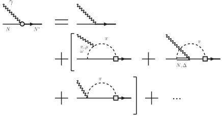
Figure 10: Graphical representation of the dressed $\bar{\Gamma}_{\gamma N\rightarrow N^{*}}$ defined by Eqs.(104)-(105)

6 Results

With the formulation presented in the above two sections, very extensive data of $\pi N$, $\gamma N$, $N(e,e^{\prime})$ and also $N(\nu_{\mu},\mu\pi)$ reactions have been analyzed. Most detailed results[4, 5, 6, 7] are for the $\Delta(1232)$ state. These will be reviewed in subsection 6.1 for the electromagnetic $\gamma N\rightarrow\pi N$ and $N(e,e^{\prime}\pi)$ processes and 6.2 for the weak $N(\nu_{\mu},,\mu\pi)$ reactions. The investigation of higher mass $N^{*}$ states began in 2006 and is still in the progressing stage. Thus only limited results will be reviewed in subsection 6.3.

6.1 Electromagnetic Excitation of the $\Delta(1232)$ state

The electromagnetic excitation of the $\Delta(1232)$ state was studied in Refs. [4, 5, 9]. The main objective was to extract the $\gamma N\rightarrow\Delta(1232)$ form factors from the data of photoproduction and electroproduction of $\pi$ in the invariant mass $W\leq$ 1.3 GeV region where only $\pi N$ and $\gamma N$ channels are open. Thus it was studied by using the formula presented in section 4 by keeping only one bare $\Delta$ state and including only the $\pi N$ and $\gamma N$ channels. The resulting model is identical to the model developed in Refs.[4] (called the Sato-Lee (SL) model in the literatures).

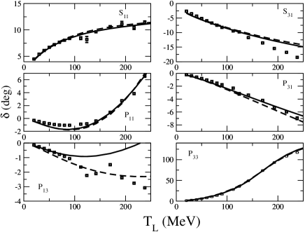
Figure 11: Phase shifts of $\pi N$ elastic scattering up to $T_{L}=$250 MeV. Solid and dotted stand for model SL and SL2 respectively. Data, $L_{2T,2J}$, are from the energy independent SAID [47] analysis plus 8 points from their energy dependent solution for the $P_{13}$ and $P_{31}$ partial waves at lower energies.

The $\gamma N\rightarrow\Delta$ (1232) form factor $\Gamma_{\Delta,\gamma N}$ is parametrized in the form developed by Jones and Scadron [46]. With the normalization $<{\vec{k}}|{\vec{k}^{\prime}}>=\delta({\vec{k}}-{\vec{k}^{\prime}})$ for the plane wave states and $<\phi_{B}|\phi_{B^{\prime}}>=\delta_{B,B^{\prime}}$ for $B=N$ and bare $\Delta$ states, the covariant form of Jones and Scadron can be cast, in the rest frame of the $\Delta$ and for the photon momentum $q=(\omega,\vec{q})$, as

$$<m_{j_{\Delta}},m_{t_{\Delta}}|\Gamma_{\Delta,\gamma N}(q)|\lambda_{\gamma}\lambda_{N},m_{t_{N}}>$$

$$=F\times\langle{\textstyle{3\over 2}}m_{t_{\Delta}}|{\textstyle{1\over 2}}1m_{t_{N}}0\rangle$$

$$\,\,\,\,\,\times[M_{m_{j_{\Delta}},\lambda_{\gamma}\lambda_{N}}(q)G_{M}(Q^{2})+E_{m_{j_{\Delta}},\lambda_{\gamma}\lambda_{N}}(q)G_{E}(Q^{2})+C_{m_{j_{\Delta}},\lambda_{\gamma}\lambda_{N}}(q)G_{C}(Q^{2})]\,,$$ (106)

where $<jm|j_{1},j_{2},m_{1},m_{2}>$ is the Clebsch-Gordon coefficient of $\vec{j}_{1}+\vec{j}_{2}=\vec{j}$ coupling, $\lambda_{\gamma}$ and $\lambda_{N}$ are the helicities of the initial photon and nucleon, $m_{j_{\Delta}}$ is the z-component of the $\Delta$ spin, $m_{t_{\Delta}}$ and $m_{t_{N}}$ denote the isospin components. In Eq.(106) we have defined

$$F=\frac{-e}{(2\pi)^{3/2}}\sqrt{\frac{E_{N}(\vec{q})+m_{N}}{2E_{N}(\vec{q})}}\frac{1}{\sqrt{2\omega}}\frac{3(m_{\Delta}+m_{N})}{4m_{N}(E_{N}(\vec{q})+m_{N})}\,,$$ (107)

and the excitation kinematics are contained in

$$M_{m_{j_{\Delta}},\lambda_{\gamma}\lambda_{N}}(q) = <m_{j_{\Delta}}|i\vec{S}\times\vec{q}\cdot\vec{\epsilon}_{\lambda_{\gamma}}|\lambda_{N}>\,,$$ (108)

$$E_{m_{j_{\Delta}},\lambda_{\gamma}\lambda_{N}}(q) = <m_{j_{\Delta}}|\vec{S}\cdot\vec{\epsilon}_{\lambda_{\gamma}}\vec{\sigma}\cdot\vec{q}+\vec{S}\cdot\vec{q}\vec{\sigma}\cdot\vec{\epsilon}_{\lambda_{\gamma}}|\lambda_{N}>\,,$$ (109)

$$C_{m_{j_{\Delta}},\lambda_{\gamma}\lambda_{N}}(q) = \frac{1}{m_{\Delta}}<m_{j_{\Delta}}|\vec{S}\cdot\vec{q}\vec{\sigma}\cdot\vec{q}\epsilon_{0}|\lambda_{N}>\,,$$ (110)

where $e=\sqrt{4\pi/137}$, photon polarization vector is defined by $\vec{\epsilon}_{\pm 1}=\mp\frac{1}{\sqrt{2}}(\hat{x}\pm i\hat{y})$, and $\epsilon^{0}_{\pm 1}=0$ for $\lambda_{\gamma}=\pm 1$, $\vec{\epsilon}_{0}=0$ and $\epsilon^{0}_{0}=1$ for the scalar component $\lambda_{\gamma}=0$. The transition spin $\vec{S}$ is defined by $<j_{\Delta}m_{\Delta}|S_{m}|j_{N}m_{N}>=<j_{\Delta}m_{\Delta}|j_{N}1m_{N}m>$.

The form factors $G_{M}(Q^{2})$, $G_{E}(Q^{2})$, and $G_{C}(Q^{2})$ in Eq.(106) describe magnetic M1, Electric E2, and Coulomb C2 transitions. Choosing the photon direction $\vec{q}$ in the z-direction, the above form factors are related to the form factors in helicity representation defined in Eqs.(97)-(99), which are consistent with the convention of Particle Data Group [1] (PDG)

$$A_{3/2}(Q^{2}) = -\frac{\sqrt{3}A}{2}[G_{M}(Q^{2})+G_{E}(Q^{2})]\,,$$ (111)

$$A_{1/2}(Q^{2}) = -\frac{A}{2}[G_{M}(Q^{2})-3G_{E}(Q^{2})]\,,$$ (112)

$$S_{1/2}(Q^{2}) = -\frac{|\vec{q}|A}{\sqrt{2}m_{\Delta}}G_{C}(Q^{2})\,,$$ (113)

with

$$A = \frac{e}{2m_{N}}\sqrt{\frac{m_{\Delta}}{m_{N}K_{\gamma}}}\frac{|\vec{q}|}{1+Q^{2}/(m_{N}+m_{\Delta})^{2}}\,,$$ (114)

where $K_{\gamma}=\frac{m_{\Delta}^{2}-m_{N}^{2}}{2m_{\Delta}}$.

The dressed form factor $\bar{\Gamma}_{\Delta,\gamma N}$ has the same symmetry property of the bare vertex defined above. Thus it can be expanded in the same form of Eq.(106). We denote the dressed form factors by $\bar{G}_{M}(Q^{2})$, $\bar{G}_{E}(Q^{2})$, $\bar{G}_{C}(Q^{2})$. The corresponding helicity amplitudes $\bar{A}_{\lambda}$ can also be calculated by using the same relations Eqs.(111)-(113). In Ref. [4], it was shown that $\bar{\Gamma}_{\Delta,\gamma N}$ can also be calculated from the K-matrix form of $\bar{\Gamma}_{\Delta,\gamma N}$ which is directly related to the imaginary parts of the $full$ multipole amplitudes $M_{1+}$, $E_{1+}$ and $S_{1+}$ at the resonance energy $W_{R}$ where the $\pi N$ phase shift is $90^{0}$, independent of the form of the non-resonant amplitudes. Thus the dressed ratios can be calculated from

$$\bar{R}_{EM}(W=W_{R}) = -\frac{\bar{G}_{E}}{\bar{G}_{M}}=\frac{{\rm Im}E_{1+}}{{\rm Im}M_{1+}}\,,$$ (115)

$$\bar{R}_{SM}(W=W_{R}) = \frac{|\vec{q}|}{2m_{\Delta}}\frac{\bar{G}_{C}}{\bar{G}_{M}}=\frac{{\rm Im}S_{1+}}{{\rm Im}M_{1+}}\,,$$ (116)

It is common to define $G^{*}_{M}$ for the M1 transition form factor which is related to our dressed form factor by

$$G^{*}_{M}(Q^{2})=\sqrt{\frac{\Gamma^{exp}_{\Delta}}{\Gamma^{SL}_{\Delta}}}\frac{\bar{G}_{M}(Q^{2})}{\sqrt{1+Q^{2}/(m_{\Delta}+m_{N})^{2}}}\,,$$ (117)

where $\Gamma^{exp}_{\Delta}=115$ MeV is used in extracting the data from $M^{3/2}_{1+}$ amplitude of pion electroproduction amplitude and $\Gamma^{SL}=93$ MeV from the constructed model.

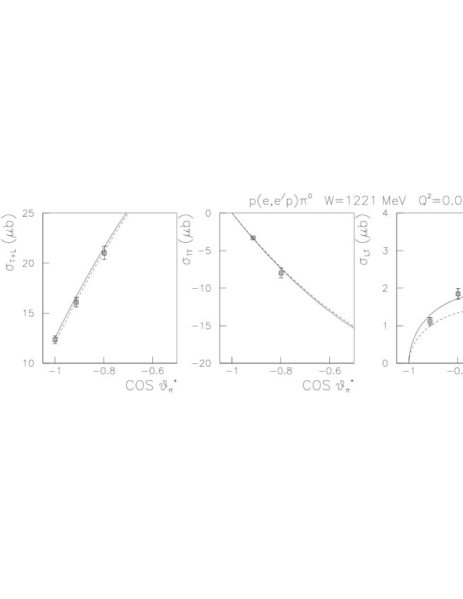
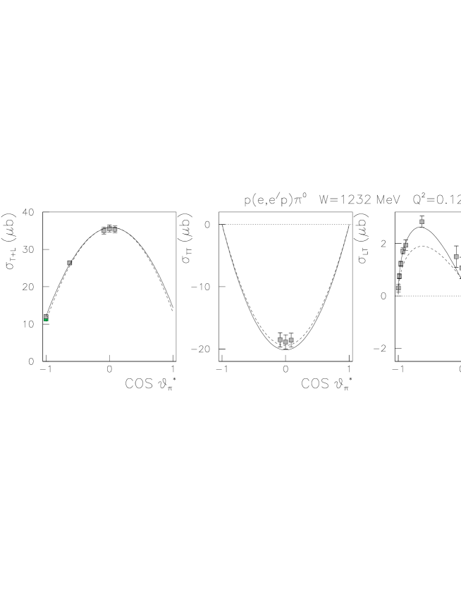
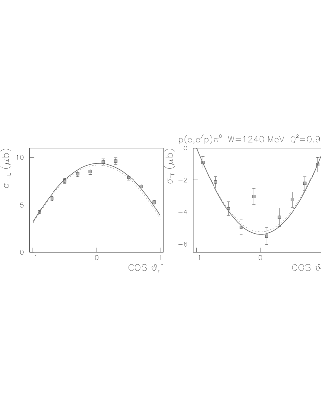
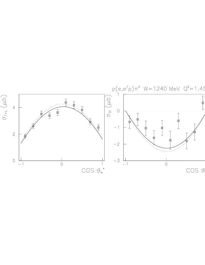
Figure 12: Fits to experimental $p(e,e^{\prime}p)\pi^{0}$ structure functions. Solid lines are from the fits with the bare form factors $G_{M}(Q^{2})$, $G_{E}(Q^{2})$ and $G_{C}(Q^{2})$ adjusted at each $Q^{2}$. The dashed curves are from the calculations using the parametrization Eqs.(118)-(119). The structure functions $\sigma_{\alpha}$ are $R^{\alpha}_{em}$ defined in Eq.(83). Data are from MAMI [48] at $Q^{2}=0.06$ GeV², BATES [49, 50, 51] at $Q^{2}=0.127$ GeV², CLAS [52] ($W=1220$ MeV) and MAMI [53] ($W=1221$ MeV) at $Q^{2}=0.2$ GeV² and CLAS [54] at $Q^{2}=0.9,1.45$ GeV².

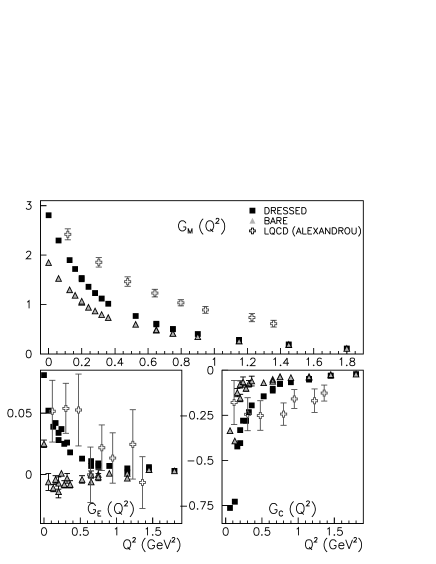
Figure 13: The extracted $\gamma N\rightarrow\Delta$ form factors. Dark squares(triangles) are the dressed (bare) values. Open crosses with errors are the lattice QCD calculation of Ref. [55, 56].

With the above definitions of $\gamma N\rightarrow\Delta$ (1232) form factors, we now describe the results obtained in Refs.[4, 5, 9]. The first step in extracting the $\gamma N\rightarrow\Delta$ (1232) form factors is to fix the hadronic parameters by fitting the $\pi N$ elastic scattering up to $W=$ 1.3 GeV. Two fits from Refs. [4, 9] are shown in Fig.11. These two models will be called SL and SL2 models in later discussions. Their differences are mainly in fitting the weak $P_{13}$ partial waves. These two fits provide us with an opportunity to examine the model dependence of the extracted $\gamma N\rightarrow\Delta$ (1232) form factors.

The next step is to adjust the bare $\gamma N\rightarrow\Delta$ (1232) form factors $G_{M}(Q^{2})$, $G_{E}(Q^{2})$, and $G_{C}(Q^{2})$ to fit the world data of $\gamma p\rightarrow\pi^{0}p,\pi^{+}n$ , $p(e,e^{\prime}\pi^{0})p$ and $p(e,e^{\prime}\pi^{+})n$. In Fig.12, we show some typical fits to the structure functions of $p(e,e^{\prime}\pi^{0})p$ . The resulting bare (solid triangles) and dressed (solid squares) form factors are shown in Fig.13. In the same figure we also show the LQCD results (open crosses with errors) which are obtained from applying a chiral extrapolation procedure to get results in the physical region from the calculations with very large quark masses. We see that LQCD results agree only very qualitatively with either the extracted dressed or bare form factors. There are several difficulties in interpreting these results, as discussed by Pascalutsa and Vanderhaeghen [57]. First, the chiral extrapolation is only valid for low $Q^{2}$, although it has been used in a rather high $Q^{2}$ region. Second, there are higher order corrections on the commonly used chiral extrapolation, which have not been under control. Thus it is not clear what to conclude from Fig. 13 for the results from LQCD of Ref. [55, 56]. Further investigations are clearly needed.

	$\bar{R}_{EM}$(%)				$\bar{R}_{SM}$(%)
$Q^{2}$		UIM	SL	SL2		UIM	SL	SL2
0.16		-1.94(0.13)	-2.45(0.2)	-2.57(0.2)		-4.64(0.19)	-4.44(0.35)	-4.36(0.35)
0.20		-1.68(0.18)	-2.21(0.2)	-2.31(0.2)		-4.62(0.18)	-4.23(0.35)	-4.14(0.35)
0.24		-2.14(0.14)	-2.70(0.2)	-2.76(0.2)		-4.60(0.28)	-4.32(0.35)	-4.21(0.35)
0.28		-1.69(0.27)	-1.99(0.2)	-2.07(0.2)		-5.50(0.31)	-5.08(0.35)	-4.97(0.35)
0.32		-1.59(0.17)	-2.29(0.2)	-2.35(0.2)		-5.71(0.33)	-4.87(0.35)	-4.75(0.35)
0.36		-1.52(0.27)	-1.80(0.2)	-1.82(0.2)		-5.79(0.43)	-4.76(0.35)	-4.56(0.35)

Table 1: Extracted values of $E2/M1$ ratio $\bar{R}_{EM}$ and $C2/M1$ ratio $\bar{R}_{SM}=S_{1+}/M_{1+}$ at $Q^{2}=0.16-0.36$ GeV² from analysis of results from a CLAS measurement [52] of the $p(e,e^{\prime}p)\pi^{0}$ reaction. Methods used are Unitary Isobar Model (UIM) and the SL and SL2 which use hadronic parameters determined in Ref.[4] and Ref.[9], respectively. Errors are statistical only.

Figure 14: Magnetic dipole transition form factor $G^{*}_{M}$ for $\gamma^{*}N\rightarrow\Delta(1232)$, normalized to the proton dipole form factor $G_{D}(Q^{2})=1/[1+Q^{2}/\Lambda^{2}]^{2}$ with $\Lambda^{2}=0.71$ (GeV/c)². Experimental points are analyses of inclusive data ($\bigcirc$) from pre-1990 experiments at DESY and SLAC [58, 59, 60, 61] and recent exclusive $p(e,e^{\prime}p)\pi^{o}$ data (blacksquare) from BATES [49, 50, 51], MAMI [48, 53] and JLAB [52, 54, 62, 63, 64, 65]. Solid curve is from the dressed calculation of SL model using the parametrization of Eq. (119). The dotted curve is obtained when the meson cloud effect, defined by Eq.(105) is turned off.

Here we note that the extracted bare form factor $G_{M}(Q^{2})$ (solid triangles) in Fig. 13 are close to the following parametrization of Ref.[5]

$$G_{M}(Q^{2})=G_{M}(0)R_{SL}(Q^{2})G_{p}(Q^{2})\,,$$ (118)

where $G_{p}(Q^{2})=1/(1+Q^{2}/M_{V}^{2})^{2}$ with $M_{V}^{2}=0.71$ (GeV/c)² being the well determined nucleon form factor, and

$$R_{SL}(Q^{2})=(1+a\,Q^{2})\,exp(-b\,Q^{2})\,,$$ (119)

with $G_{M}(0)=1.85$, $a=0.154$ (GeV)^-2 and $b=0.166$ (GeV)^-2. By using this parametrization, the predicted bare (dotted curve) and dressed (solid curve) $G^{*}_{M}(Q^{2})$ ( defined by Eq.(117)) are compared with the available empirical values in Fig.14. It is clear that the resulting dressed $G^{*}_{M}(Q^{2})$ (solid curve) agree well with the available empirical values. The differences between the solid and dotted curves indicate that the meson cloud effects, illustrated in Fig.10, are important in the low $Q^{2}$ region and gradually diminish as $Q^{2}$ increases. This result is one of the main accomplishments of many-year study of $N$-$\Delta$ (1232) excitation, and has motivated future studies up to $Q^{2}=11$ (GeV)² with 12 GeV upgrade of CEBAF at JLab.

Historically, the $\Delta$ (1232) is described by the constituent quark model. To see the extent to which the extracted $G_{M}(Q^{2})$ form factors can be understood with this model, it is instructive to first consider the naive s-wave non-relativistic quark model within which $\mu_{p}$ for the proton magnetic moment and $\mu_{\Delta^{+}p}$ for the $\Delta^{+}$-$p$ M1 transition are defined by

$$\frac{e}{2m_{p}}\mu_{p}=\langle p,m_{s_{N}}={\textstyle{1\over 2}}|\sum_{i}\frac{e_{i}}{2m_{q}}\sigma_{i}(z)|p,m_{s_{N}}={\textstyle{1\over 2}}\rangle\,,$$ (120)

$$\frac{e}{2m_{p}}\mu_{\Delta^{+}p}=\langle\Delta^{+},m_{s_{\Delta}}={\textstyle{1\over 2}}|\sum_{i}\frac{e_{i}}{2m_{q}}\sigma_{i}(z)|p,m_{s_{N}}={\textstyle{1\over 2}}\rangle\,.$$ (121)

From the above relation and the definition Eq.(106), one observes that the magnetic M1 form factor of $\gamma N\rightarrow\Delta$ at $Q^{2}=0$ can be directly calculated from the proton magnetic moment

$$G_{M}(0) = [\sqrt{2}G_{p}(0)]\left[\frac{2(E_{N}(q)+m_{N})}{3(m_{\Delta}+m_{N})}\right]\sqrt{\frac{2E_{N}(q)}{E_{N}(q)+m_{N}}}=0.84\mu_{p}\,.$$ (122)

where $q=(m^{2}_{\Delta}-m^{2}_{N})/2m_{\Delta}\sim 260$ MeV/c. If we use the empirical value of proton magnetic moment $\mu_{p}\rightarrow\mu^{exp}_{p}=1+\kappa_{p}\sim 2.77$, we then find $G_{M}(0)\sim 2.32$ which is considerably smaller than the extracted dressed value $\sim 3.2$ seen in Fig. 13. This was observed in Ref.[4] and interpreted as due to the large meson cloud effects which are the difference between the solid and dotted curves in Fig.14.

We thus observe that extracted bare value $G_{M}(0)=1.85$ can perhaps be understood in terms of constituent quark degrees of freedom if we tune properly the constituent quark model calculations. On the other hand, our extracted bare E2 transition form factor $G_{E}(0)$ cannot be understood within the non-relativistic constituent quark model. With the tensor force within the conventional one-gluon-exchange, the estimated E2 transition of $\gamma N\rightarrow\Delta$ is known to be negligibly small compared with the value calculated from our value $G_{E}(0)=-0.025$. In Ref.[9], the extracted form factors are also compared with relativistic constituent quark models. Only qualitative agreement is obtained.

We next present our determined dressed $\bar{R}_{EM}$ and $\bar{R}_{SM}$ in the low $Q^{2}$ region where very large meson cloud effects have been identified in Fig. 13. Our results, SL and SL2, are listed in table 1 and compared with the values determined using the unitary isobar model (UIM). The differences between our values and that from the UIM reflect some model-dependence in the extraction. Here we note that only the data of five of the eleven $N(e,e^{\prime}\pi)N$ independent observables were available and used in the fits. Thus the differences between different models shown in Table 1 are surprisingly small. So far there is no satisfactory theoretical understanding of the results of $\bar{R}_{EM}$ and $\bar{R}_{SM}$ shown in Table 1.

Figure 15: Total cross sections of $N(\nu_{\mu},\mu^{-}\pi)N$ reactions predicted by the SL Model[6]. The data are from Ref.[71]. The solid curves are from full calculations. The dotted curves are from turning off pion cloud effects on N-$\Delta$ transitions. The dashed curves are the contributions from the non-resonant amplitude.

6.2 Weak excitation of the $\Delta$ state

The model developed in Refs.[4, 5], the SL model, was extended to investigate neutrino-induced pion production reactions. The extension is tedious but straightforward, as detailed in Refs.[6, 7]. Here we just focus on the extraction of the weak $N$-$\Delta$ (1232) form factor which has vector ($V$) and axial vector ($A$) components. The vector current matrix element $<\Delta\mid V^{\mu}\mid N>$ can be obtained from the SL model by appropriate isospin rotations. The most general form of the axial vector current matrix element is well known, as given in Refs.[66, 67, 68]. To see how it is different from the electromagnetic excitation given in Eqs.(106) - (109), we cast[6] it in the rest frame of a $\Delta$ on the resonance energy( $p_{\Delta}=(m_{\Delta},\vec{0}),p_{N}=(E_{N}(q),-\vec{q}),q=(m_{\Delta}-E_{N}(q),\vec{q}))$ as

$$<\Delta|\vec{A}^{i}|N> = \sqrt{\frac{E_{N}+m_{N}}{2m_{N}}}[(d_{1}+\frac{m_{\Delta}^{2}-m_{N}^{2}}{m_{N}^{2}}d_{2})\vec{S}$$ (123)

$$-(d_{2}+d_{3})\frac{(\vec{S}\cdot\vec{q})\vec{q}}{m_{N}^{2}}-id_{4}\frac{\vec{S}\times\vec{q}(\vec{\sigma}\cdot\vec{q})}{m_{N}^{2}(E_{N}+m_{N})}]T^{i},$$

$$<\Delta|A^{0i}|N> = \sqrt{\frac{E_{N}+m_{N}}{2m_{N}}}[d_{2}\frac{\vec{S}\cdot\vec{q}(m_{\Delta}+E_{N})}{m_{N}^{2}}$$ (124)

$$-d_{3}\frac{\vec{S}\cdot\vec{q}(m_{\Delta}-E_{N})}{m_{N}^{2}}]T^{i},$$

where $T^{i}$ is the $i-$th component of the isospin transition operator(defined by the reduced matrix element $<3/2\mid\mid{\vec{T}}\mid\mid 1/2>=-<1/2\mid\mid{\vec{T}}^{+}\mid\mid 3/2>=2$ in Edmonds convention[69]), and the transition spin $\vec{S}$ is defined by the same reduced matrix elements of ${\vec{T}}$. The above expression suggests that $d_{1},d_{2}$ terms describe the Gamow-Teller transition and $d_{4}$ describes the quadrupole transition. For simplicity, we follow Ref.[68] to fix the form factors $d_{i}(q^{2})$ at $q^{2}=0$ using the non-relativistic constituent quark model. The axial vector current operator for a constituent quark is derived from taking the non-relativistic limit of the standard form $g_{Aq}\bar{q}\gamma^{\mu}\gamma_{5}\frac{\tau}{2}q$. By some derivations[6], we find that

$$d_{1}(Q^{2}_{0}) = g^{*}_{A}(Q^{2}_{0})(1+\frac{m^{2}_{\Delta}-m^{2}_{N}}{2m_{N}(m_{\Delta}+m_{N})})\,,$$ (125)

$$d_{2}(Q^{2}_{0}) = -g^{*}_{A}(Q^{2}_{0})\frac{m_{N}}{2(m_{\Delta}+m_{N})}\,,$$ (126)

$$d_{3}(Q^{2}_{0}) = -g^{*}_{A}(Q^{2}_{0})\frac{m^{2}_{N}}{q^{2}-m_{\pi}^{2}}\,,$$ (127)

where $g_{A}^{*}(Q^{2}_{0})=\frac{1}{\sqrt{2}}\frac{6}{5}g_{A}$ with $g_{A}=1.26$ and $Q_{0}^{2}=(m_{\Delta}-m_{N})^{2}$. This agrees with the results of Ref.[68] if we neglect the difference between $m_{N}$ and $m_{\Delta}$.

To account for the $q^{2}$-dependence, we assume that

$$d_{i}(Q^{2})=d_{i}(0)R_{SL}(Q^{2})G_{A}(Q^{2})\,,$$ (128)

where $R_{SL}(Q^{2})$ is defined in Eq.(119) and has been determined in the study of $\gamma N\rightarrow\Delta$ (1232) form factor, and $G_{A}(Q^{2})=1/(1+Q^{2}/M^{2}_{A})^{2}$ with $M_{A}=1.02$ GeV is the nucleon axial form factor[70].

With the axial form factors defined above, our calculations of $p(\nu_{\mu},\mu\pi)N$ do not involve any adjustment of the parameters, since all of the the parameters of the non-resonant amplitudes and the vector part of the $N$-$\Delta$ transition form factor have been completely fixed in the study of electromagnetic pion production. The predicted total cross sections are compared with with the data[71] in Fig.15. We see that the predictions(solid curves) agree reasonably well with the data for three pion channels. For the data on neutron target, our predictions(solid curves in the middle and lower figures) are in general lower than the data. This is perhaps related to the procedures used in Ref.[71] to extract these data from the experiments on deuteron target.

Similar to the electromagnetic $N$-$\Delta$ transition, we have also found significant meson cloud effects on the axial $N$-$\Delta$ transition form factor. This is also shown in Fig.15. We see that our full calculations(solid curves) are reduced significantly to dotted curves if we turn off the dynamical pion cloud effects. If we further turn off the contributions from bare N-$\Delta$ transitions, we obtain the dashed curves which correspond to the contributions from the non-resonant amplitudes. Clearly, the non-resonant amplitudes are weaker, but are also essential in getting the good agreement with the data since they can interfere with the resonant amplitudes.

Figure 16: Differential cross sections $d\bar{\sigma}/dQ^{2}$ of $p(\nu_{\mu},\mu^{-}\pi^{+})p$ reaction averaged over neutrino energies 0.5 GeV $<E_{\nu}<$ 6 GeV. The curves are the predictions of the SL Model[6]. The dotted curve(dot-dashed curve) is the contribution from axial vector current A (vector current V). The solid curve is from the full calculations with V-A current. The data are from Ref.[71].

In Fig.16 we compare the $Q^{2}$-dependence of the differential cross sections $d\sigma/dQ^{2}$ with the data from ANL[71]. We see that our predictions(solid curve) agree reasonable well with the data both in magnitude and $Q^{2}-$dependence. In Fig.16 we also compare the contributions from vector current(dot-dashed curve) and axial vector current(dotted curve). They have rather different $Q^{2}$-dependence in the low $Q^{2}$ region and interfere constructively with each other to yield the solid curve of the full results. Since vector current contributions are very much constrained by the $(e,e^{\prime}\pi)$ data, the results of Fig.16 suggest that the constructed axial vector currents are consistent with the data.

The extraction of the axial $N$-$\Delta$ form factor is much more difficult because the lack of sufficient data. The dressed (solid curve) and bare (dotted curve) axial $N$-$\Delta$ form factors are shown in the right-hand side of Fig.17. Clearly, their $Q^{2}$-dependence is weaker than the $\gamma N\rightarrow\Delta$ form factors which are discussed in the previous subsection and also displayed in left hand side of Fig.17. However, the meson cloud effects, the difference between the solid and dotted curves, are comparable in both form factors.

The axial $N$-$\Delta$ form factor was determined in previous analysis. In Fig.18, we see that our results (solid) are significantly different from the previous results( dot-dashed curve) at high $Q^{2}$. Obviously, more experimental data are needed to resolve the differences. With the new world-wide effort in developing next-generation neutrino experiments, progress in this direction is expected in the near future.

Figure 17: The N-$\Delta$ form factors: left panel: Magnetic M1 form factors given in Ref.[5], right panel: axial vector form factor determined in Ref.[6]. The solid curves are from full calculations. The dotted curves are obtained from turning off the pion cloud effects. $G_{D}=1/(1+Q^{2}/M^{2}_{V})^{2}$ with $M_{V}=0.84$ GeV is the usual proton dipole form factor and $G_{A}=1/(1+Q^{2}/M^{2}_{A})^{2}$ with $M_{A}=1.02$ GeV is the axial nucleon form factor of Ref. [70].

Figure 18: Compare the dressed axial N-$\Delta$ form factor predicted by the Model of Ref.[6] (solid curve) with the empirical form factor(dot-dash curve) determined in Ref.[72].

6.3 Excitations of higher mass $N^{*}$ states

To investigate higher mass $N^{*}$ states up to invariant mass $W=2$ GeV, we apply the full model developed in sections 3 and 4. The meson-baryon (MB) channels considered are $\gamma N,\pi N,\eta N$ and the $\pi\pi N$ channel which has resonant $\pi\Delta,\sigma N,\rho N$ components. The resonant amplitude $t^{R}_{M^{\prime}B^{\prime},MB}$ of Eq.(48) are generated by including one or two bare $N^{*}$ states in each partial waves. Clearly it is a highly nontrivial task to extract the resonance parameters from solving this multi-channels multi-resonance problem. It requires simultaneous fits to all available data of $\pi N$, $\gamma N$, and $N(e,e^{\prime})$ data with all possible two-particle and three-particle $\pi\pi N$ states. This ambitious work started in 2006 at the Excited Baryon Analysis Center (EBAC) of JLab, and is still progressing rapidly. Thus the results reviewed in this subsection are only the first-step results which will be refined when all of the world’s meson production data of $\pi N$, $\gamma N$, and $N(e,e^{\prime})$ reactions are included in the analysis.

6.3.1 $\pi N$ scattering

Similar to the study of the $\Delta$ (1232) state, the first step to investigate higher mass $N^{*}$ states is to determine the hadronic parameters by fitting the data of $\pi N$ elastic scattering. Such a fit was obtained in Ref.[10] by assuming one or two bare $N^{*}$ states in each of $S$, $P$, $D$, and $F$ partial waves . The $\pi N$ scattering amplitudes of isospin $T=1/2$ predicted by the resulting model, the JLMS model, are compared with the empirical values of SAID[47] in Fig.19. Similar good agreement is also found for the $T=3/2$ partial waves, as also given in Ref.[10]. The corresponding good agreement with the data of differential cross sections and polarization observable $P$ are illustrated in Fig.20 for some of the data. The predicted total cross sections are also in good agreement with the data as shown in Fig.21.

The resulting parameters of 21 bare $N^{*}$ states, presented in Ref.[10], is the starting point for performing a dynamical coupled-channel analysis of the world’s meson production data of $\pi N$, $\gamma N$, and $N(e,e^{\prime})$ reactions. In the next three subsections, we review the results obtained so far. Here we also mention that it is necessary to develop an analytic continuation method to identify the nucleon resonances with the poles of the scattering amplitudes on complex energy plane. This has been developed[14], but will not be discussed here because of its technical complexities.

   

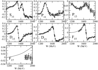
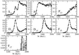
Figure 19: The $\pi N$ partial wave amplitudes of isospin $T=1/2$ calculated from the JLMS model[10] are compared with the energy independent solutions of Ref. [47]. Left (right) panel is for real (imaginary) parts of the amplitudes

6.3.2 $\pi N\rightarrow\pi\pi N$ reactions

The main difficulty in fitting the $\pi N$ elastic scattering data, described above, is that the model contains many parameters mainly due to the lack of sound theoretical guidance in parametrizing the bare $N^{*}\rightarrow\pi N,\eta N,\pi\Delta,\rho N,\sigma N$ form factors. Thus it is necessary to examine these $N^{*}$ parameters; in particular the parameters associated with the unstable $\pi\Delta$, $\rho N$, and $\sigma N$ channels. This has been done in Ref.[13] in the study of $\pi N\rightarrow\pi\pi N$ reactions which are known to be dominated by these unstable particle channels.

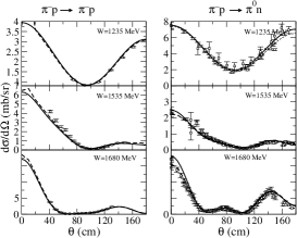
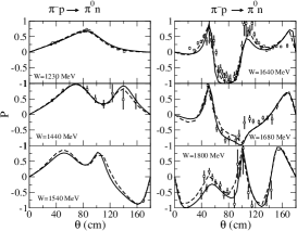
Figure 20: Differential cross sections $d\sigma/d\Omega$ (left) and asymmetry $P$ (right) of $\pi^{-}p\rightarrow\pi^{-}p,\pi^{0}n$ reactions. The solid curves are from JLMS model[10].

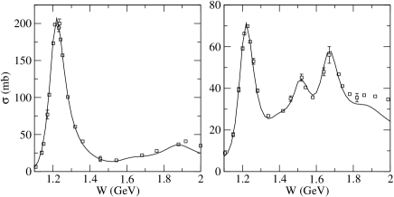
Figure 21: Total cross sections of $\pi^{+}p$ (left) and $\pi^{-}p$ (right) reactions. Solid curves are from the JLMS model[10]. Only few data are shown for a clear comparison between curves. The data are from Refs. [1, 73].

Before we present the predicted $\pi N\rightarrow\pi\pi N$ cross sections, we note here that the main feature of our approach is a dynamical coupled-channels treatment of the unstable $\pi\Delta,\rho N,\sigma N$ channels. This effect can be explicitly seen by writing the coupled-channels equations, Eq.(57), as

$$t_{MB,\pi N}(E)=\sum_{M^{{}^{\prime}}B^{{}^{\prime}}}[1-vG]^{-1}_{MB,M^{{}^{\prime}}B^{{}^{\prime}}}v_{M^{{}^{\prime}}B^{{}^{\prime}},\pi N}\,,$$ (129)

where $MB=\pi\Delta,\rho N,\sigma N$, and the intermediate meson-baryon states can be $M^{{}^{\prime}}B^{{}^{\prime}}=\pi N,\eta N,\pi\Delta,\sigma N,\rho N$. The predicted $\pi N\rightarrow\pi\pi N$ total cross sections depend on the coupled-channel effects due to these intermediate $M^{\prime}B^{\prime}$ states,

The results for $\pi N\rightarrow\pi\pi N$ total cross sections are shown in Fig.22. We see that our full calculations (solid curves) can reproduce the data to a very large extent for all possible $\pi\pi N$ final states up to $W=2$ GeV. These results are far more successful than all of the previous investigations, as discussed in Ref.[13]. When only the term with $M^{\prime}B^{\prime}=MB$ in the Eq.(129) and in $\bar{\Gamma}_{N^{*}\rightarrow MB}$ of Eqs.(52)-(53) is kept, the calculated total cross sections (solid curves) are changed to the dotted curves in Fig.22. If we further neglect the coupled-channels effects by setting $t_{\pi N,MB}=v_{\pi N,MB}$, we then get the dashed curves which are very different from the full calculations (solid curves), in particular in the high $W$ region. Clearly coupled-channel effects are very large.

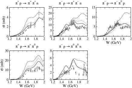
Figure 22: The coupled-channels effects on $\pi N\rightarrow\pi\pi N$ reactions. The solid curves are from full calculations, the dotted curves are from keeping only $M^{\prime}B^{\prime}=MB$ in the Eq.(129) and in $\bar{\Gamma}_{N^{*}\rightarrow MB}$ of Eqs.(52)-(53), the dashed curves are from setting $t_{MB,M^{\prime}B^{\prime}}=v_{MB,M^{\prime}B^{\prime}}$. The data are from [74].

The results shown in Fig.22 indicate that the $N^{*}\rightarrow\pi\Delta,\rho N,\sigma N$ determined from fitting $\pi N$ elastic scattering data are reasonable, but clearly need to be improved. To make the progress in this direction, it is necessary to have more complete data of $\pi N\rightarrow\pi\pi N$ reactions from new hadron facilities such as J-PARC. Hopefully, this can be realized in the near future. At the present time, we have to rely on recent data of $\gamma N\rightarrow\pi\pi N$ to refine the $N^{*}\rightarrow\pi\Delta,\rho N,\sigma N$ parameters. Effort in this direction is being made at EBAC.

6.3.3 Electromagnetic pion production reactions

The fits to $\pi N$ reaction data, presented in the previous two subsections, have fixed all of the hadronic parameters of the effective Hamiltonian Eqs.(39)-(43). Most of the electromagetic parameters associated with the nonresonant $\gamma N\rightarrow\pi N$ are also known from previous investigation of $\Delta$ (1232) state. Thus the bare helicity amplitudes, $A_{3/2}$, $A_{1/2}$, and $S_{1/2}$, defined in Eqs.(97)-(99), are the main unknown parameters in our investigations of electromagnetic pion production reactions. The first step in determining these helicity amplitudes had been completed in Ref.[11] by performing $\chi^{2}-$fits to the available photoproduction data of $\gamma N\rightarrow\pi N$ reactions up to $W=1.65$ GeV. The quality of the resulting fit can be seen in Figs. 23 for the $\gamma p\rightarrow\pi^{0}p$. Similar good agreement was also obtained for the $\gamma p\rightarrow\pi^{+}n$, as also presented in Ref.[11].

Clearly, the fit to the data needs to be improved, but is sufficient for revealing the coupled-channels effects in a dynamical approach. In electromagnetic pion productions, the coupled-channel effects are in the loop integrations over the intermediate meson-baryon states $MB$ in the following expressions for the non-resonant amplitudes and the dressed $\gamma N\rightarrow N^{*}$ vertex

$$t_{\pi N,\gamma N}=v_{\pi N,\gamma N}+\sum_{MB}t_{\pi N,MB}G_{MB}v_{MB,\gamma N}\,,$$ (130)

$$\bar{\Gamma}_{N^{*},\gamma N}={\Gamma}_{N^{*},\gamma N}+\sum_{MB}\bar{\Gamma}_{N^{*},MB}G_{MB}v_{MB,\gamma N}\,.$$ (131)

We show the coupled-channels effects on the total cross sections of $\gamma p\rightarrow\pi^{0}p,\pi^{+}n$ in Fig. 24. We see that the calculated total cross sections (solid curves) are in good agreement with the data. The dashed curves are obtained when the channels $MB=\eta N$, $\pi\Delta$, $\rho N$, and $\sigma N$ are turned off in the loop integrations of Eqs.(130)-(131). Clearly, the coupled-channels effects $\gamma N\rightarrow\eta N$, $\pi\Delta$, $\rho N$, $\sigma N$ $\rightarrow\pi N$ can change the cross sections by about 10 - 20 $\%$ in the $\Delta$ (1232) region and as much as 50 $\%$ in the $W>$1400 MeV second resonance region.

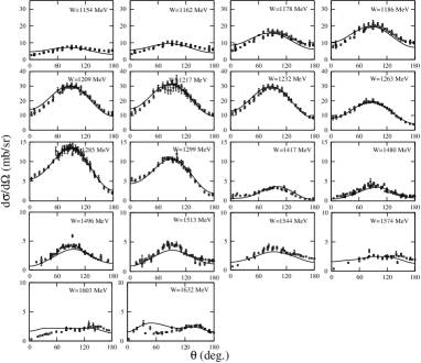
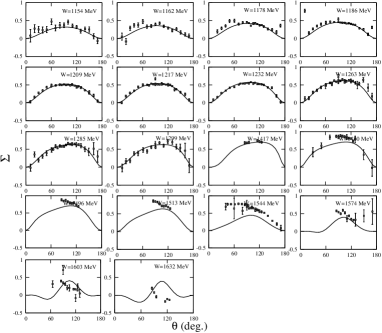
Figure 23: Differential cross section $d\sigma/d\Omega$ (upper) and photon asymmetry $\Sigma_{\gamma}$ (lower) for $\gamma p\rightarrow\pi^{0}p$ calculated from JLMSS model[11] are compared to experimental data obtained from Ref. [47].

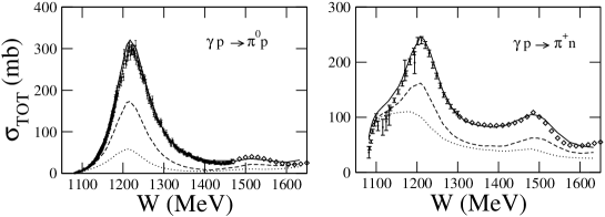
Figure 24: Total cross sections from JLMSS model[11]. The dashed curves are obtained from turning off all $MB$ channels except the $\pi N$ channel in the the loop integrations in the non-resonant amplitude and the dressed $\gamma N\rightarrow N^{*}$ vertex. The dotted curve is obtained by neglecting the off shell effects in the $\pi N$ only calculation. Experimental data are from Ref. [47].

The meson cloud effects, as illustrated in Fig.10, on several low-lying nucleon resonances are also investigated in Ref.[11]. In general, the resonance parameters must be rigorously defined by the poles on the unphysical sheet of complex energy plane. This is still being pursued[14]. Here we only illustrate the meson cloud effect on the $\gamma N\rightarrow\pi N$ multipoles for the $D_{13}$ partial wave. The results are shown in Fig.25. We see that the predicted multipole amplitudes agree well with the empirical values of SAID[47], and show typical resonant shape at $W\sim 1.5$ GeV. Our model thus also has identified a resonance at position close to the $N^{*}(1520,D_{13})$ listed by PDG. If we turn off the meson cloud effects on the $\gamma N\rightarrow N^{*}$ in this partial wave, we then get the dashed curve. Clearly, meson cloud effects are very large.

The results reviewed in this subsection are from the very first step of performing a dynamical coupled-channel analysis of $\pi$ photoproduction and electroproduction reactions up to $W=2$GeV. In parallel, the investigation of $\pi N\rightarrow\pi\pi N$ described in subsection 5.2 has also been extended to investigate $\gamma^{*}N\rightarrow\pi\pi N$ reactions. Only when the world’s data of $\pi N,\gamma^{*}N\rightarrow\pi N,\pi\pi N$ are all included in the analysis, we can establish the $N^{*}$ spectrum and their decay properties with confidence. Progress in this is being made at EBAC.

Figure 25: The predicted $\gamma N\rightarrow\pi N$ multipole amplitudes in $D_{13}$ are compared with the empirical values of SAID[47].

7 Summary and future developments

In this article, we have reviewed the dynamical model developed in Refs. [4, 5, 6, 7, 8, 9, 10, 11] for investigating the excitations of $N^{*}$ states in $\pi N$, $\gamma N$ and $N(e,e^{\prime}\pi)$ reactions. The model Hamiltonian was constructed by using a unitary transformation method, and had been used to construct a multi-channels and multi-resonances reaction model. The channels considered are $\gamma N$, $\pi N$, $\eta N$, and $\pi\pi N$ which has resonant $\pi\Delta$, $\rho N$, and $\sigma N$ channels. The resonant amplitudes are generated from 21 bare $N^{*}$ states which are renormalized by meson-baryon scattering as required by the unitary condition. The model is reduced to the well-studied Sato-Lee (SL) model when only one bare $\Delta$ state and $\pi N$ and $\gamma N$ channels are kept in the formulation.

The detailed investigations[4, 5, 6, 7] of the $\Delta$ (1232) have determined the electromagnetic $\gamma N\rightarrow\Delta$ (1232) and the axial $AN\rightarrow\Delta$ (1232) form factors. The meson cloud effects on these form factors are found to be very large in the low $Q^{2}$ region and decreases with $Q^{2}$. These form factors can be considered along with the nucleon form factors as benchmark data for testing the predictions from hadron models with effective degrees of freedom and LQCD.

The investigation of higher mass $N^{*}$ states is based on the full model presented in sections 3 and 4. The $N^{*}$ parameters can be reliably determined only when all of the available data of $\pi N$, $\gamma N$ and $N(e,e^{\prime})$ reactions with all possible two-particle and $\pi\pi N$ final states are fitted simultaneously. This ambitious work, started in 2006 at EBAC, has been progressing well to obtain good fits to the data of $\pi N$ elastic scattering, $\pi N\rightarrow\pi\pi N$, and $\gamma N\rightarrow\pi N$ reactions. Important coupled-channel effects have been revealed. Large meson cloud effects on $\gamma N\rightarrow N^{*}$ have also been identified. But more works are needed to establish the extracted $N^{*}$ parameters.

The current effort at EBAC is to obtain fits to the world data of $\pi N,\gamma^{*}N\rightarrow\pi N,\eta N,\pi\pi N$. Staring with the resulting $N^{*}$ parameters, we then focus on the $W\geq 1.7$ GeV region by also fitting the world data of $\pi N,\gamma^{*}N\rightarrow K\Lambda,K\Sigma,\omega N$. The numerical strategies for handling these additional channels have been developed and tested. This effort is needed to face the challenge from the complete and over complete measurements of all independent observables of the electromagnetic production of $K\Lambda,K\Sigma$ reactions. These measurements are expected to be carried out in the next few years at JLab. Similar complete experiments are also being developed at Mainz and Bonn.

To end of this article, we point out that the $\pi N$ data are very limited except the $\pi N$ elastic scattering. This could be the main source of the uncertainties of the extracted resonance parameters. It will be highly desirable, if more $\pi N$ reaction data can be obtained at new hadron facility J-PARC in Japan.

References

Appendix A Interaction Lagrangians

The expressions of the full Lagrangians for developing the multi-channel multi-resonance reaction model are given in Appendix A of Ref. [8]. In this appendix we only give the interaction Lagrangians for developing the SL model of electroweak pion production reactions. The Lagrangian with $\pi$, $\rho$, $\omega$, $N$, and $\Delta$ fields are

$$L_{\pi NN} = -\frac{f_{\pi NN}}{m_{\pi}}\bar{\psi}_{N}\gamma_{\mu}\gamma_{5}\vec{\tau}\psi_{N}\cdot\partial^{\mu}\vec{\phi_{\pi}}\,,$$ (132)

$$L_{\rho NN} = g_{\rho NN}\bar{\psi}_{N}[\gamma_{\mu}-\frac{\kappa_{\rho}}{2m_{N}}\sigma_{\mu\nu}\partial^{\nu}]\vec{\rho^{\mu}}\cdot\frac{\vec{\tau}}{2}\psi_{N}\,,$$ (133)

$$L_{\rho\pi\pi} = g_{\rho\pi\pi}[\vec{\phi_{\pi}}\times\partial_{\mu}\vec{\phi_{\pi}}]\cdot\vec{\rho}^{\mu}\,,$$ (134)

$$L_{\omega NN} = g_{\omega NN}\bar{\psi}_{N}[\gamma_{\mu}-\frac{\kappa_{\omega}}{2m_{N}}\sigma_{\mu\nu}\partial^{\nu}]{\omega^{\mu}}\psi_{N}\,,$$ (135)

$$L_{\pi N\Delta} = -\frac{f_{\pi N\Delta}}{m_{\pi}}\bar{\psi}_{\Delta}^{\mu}\vec{T}\psi_{N}\cdot\partial_{\mu}\vec{\phi_{\pi}}\,.$$ (136)

The effective Lagrangians for the lepton induced electroweak meson production reaction are given as

$$L_{eff} = \frac{4\pi\alpha}{q^{2}}(-\bar{e}\gamma^{\mu}e)j_{em,\mu}$$ (137)

$$-\frac{G_{F}\cos\theta_{c}}{\sqrt{2}}[\bar{\nu}_{e}\gamma^{\mu}(1-\gamma_{5})ej^{\dagger}_{CC,\mu}+\bar{e}\gamma^{\mu}(1-\gamma_{5})\nu_{e}j_{CC,\mu}]$$

$$-\frac{G_{F}}{\sqrt{2}}[\bar{\nu}_{e}\gamma^{\mu}(1-\gamma_{5})\nu_{e}+\bar{e}(2g_{V}^{e}\gamma^{\mu}-2g_{A}^{e}\gamma^{\mu}\gamma^{5})e]j_{NC,\mu}.$$

where $\alpha=1/137$, $G_{F}=1.1664\times 10^{-5}$ GeV^-2 and $g_{V}^{e}=-1/2+2\sin^{2}\theta_{W}$, $g_{A}^{e}=-1/2$. The Weinberg angle $\theta_{W}$ is known empirically to be $\sin^{2}\theta_{W}=0.231$ and $\cos\theta_{c}=0.974$ is the the Cabibbo-Kobayashi-Maskawa (CKM) coefficient.

The electromagnetic current ($j^{\mu}_{em}$), weak charge current ($j^{\mu}_{cc}$) and weak neutral current ($j^{\mu}_{nc}$) are written with the iso-vector vector current $V^{\mu}_{i}$, axial vector current $A^{\mu}_{i}$ and iso-scalar vector current $V^{\mu}_{is}$ as

$$j^{\mu}_{em} = V^{\mu}_{3}+V^{\mu}_{is}\,,$$ (138)

$$j^{\mu}_{cc} = (V^{\mu}_{1}+iV^{\mu}_{2})-(A^{\mu}_{1}+iA^{\mu}_{2})\,,$$ (139)

$$j^{\mu}_{nc} = (1-2\sin^{2}\theta_{W})j^{\mu}_{em}-V^{\mu}_{is}-A^{\mu}_{3}\,.$$ (140)

Here we have neglected the strangeness content of the nucleon. The iso-vector vector current$\vec{V}_{\mu}$ and iso-scalar vector current are $V_{\mu}^{is}$

$$\vec{V}_{\mu}=\bar{\psi}_{N}[F_{1V}\gamma_{\mu}-\frac{F_{2V}}{2m_{N}}\sigma_{\mu\nu}\partial^{\nu}]\frac{\vec{\tau}}{2}\psi_{N}+\vec{\phi}_{\pi}\times\partial_{\mu}\vec{\phi}_{\pi}$$

$$+\frac{f_{\pi NN}}{m_{\pi}}[(\bar{\psi}_{N}\gamma_{\mu}\gamma_{5}\vec{\tau}\psi_{N})\times\vec{\phi}_{\pi}]+\frac{g_{\omega\pi\gamma}}{m_{\pi}}\epsilon_{\alpha\mu\gamma\delta}\vec{\phi}_{\pi}(\partial^{\gamma}\omega^{\delta})\partial^{\alpha}\,,$$ (141)

$${V}^{is}_{\mu}=\bar{\psi}_{N}[F_{1S}\gamma_{\mu}-\frac{F_{2S}}{2m_{N}}\sigma_{\mu\nu}\partial^{\nu}]\frac{1}{2}\psi_{N}+\frac{g_{\rho\pi\gamma}}{m_{\pi}}\epsilon_{\alpha\mu\gamma\delta}\vec{\phi}_{\pi}\cdot(\partial^{\gamma}\vec{\rho^{\delta}})\partial^{\alpha}\,.$$ (142)

The axial vector current needed to construct our model is given as

$$\vec{A}^{\mu}=g_{A}\bar{N}\gamma^{\mu}\gamma_{5}\frac{\vec{\tau}}{2}N-f_{\rho\pi A}\vec{\rho}^{\mu}\times\vec{\pi}-F_{\pi}\partial^{\mu}\vec{\pi}.$$ (143)

Here $F_{\pi}=93$ MeV is the pion decay constant, and $g_{A}=1.26$ is the nucleon axial coupling constant. The iso-vector vector $N\Delta$ transition current are parametrized in the following form

$$\vec{V}_{\nu} = -i\bar{\psi}_{\Delta}^{\mu}\Gamma^{V}_{\mu\nu}\vec{T}\psi_{N}+(h.c.)\,.$$ (144)

The matrix element of $N\Delta$ current between an $N$ with momentum $p$ and a $\Delta$ with momentum $p_{\Delta}$ can be written explicitly as

$$\Gamma^{V}_{\mu\nu}=\frac{m_{\Delta}+m_{N}}{2m_{N}}\frac{1}{(m_{\Delta}+m_{N})^{2}-q^{2}}$$

$$\times[(G_{M}-G_{E})3\epsilon_{\mu\nu\alpha\beta}P^{\alpha}q^{\beta}$$

$$+G_{E}i\gamma_{5}\frac{12}{(m_{\Delta}-m_{N})^{2}-q^{2}}\epsilon_{\mu\lambda\alpha\beta}P^{\alpha}q^{\beta}\epsilon^{\lambda}_{\ \ \nu\alpha\delta}p_{\Delta}^{\gamma}q^{\delta}$$

$$+G_{C}i\gamma_{5}\frac{6}{(m_{\Delta}-m_{N})^{2}-q^{2}}q_{\mu}(q^{2}P_{\nu}-q\cdot Pq_{\nu})],$$ (145)

The expression for the $N\Delta$ transition axial vector current is given in Eqs. (123)-(124).

Appendix B Multipole amplitudes of the pseudoscalar meson production

Here we summarize the formula related the matrix elements $J^{\mu}_{\alpha}$ ($\alpha=em,cc,nc$) in Eqs. (85)-(92) to the CGLN amplitudes $F_{\alpha}$ and and multipole amplitudes. Recovering the spin indices of $J^{\mu}_{\alpha}$, we have

$$\chi^{\dagger}_{s^{\prime}}F_{\alpha}\chi_{s} = -\frac{m_{N}}{4\pi E}<\pi N(s^{\prime})|J^{\mu}_{\alpha}|N(s)>\epsilon_{\mu},$$ (146)

where $s,s^{\prime}$ are spin quantum number of nucleon. $F_{\alpha}$ is further written as sum of the contributions of vector and axial vector currents.

$$F_{em} = F_{em}^{V}\,,$$ (147)

$$F_{cc} = F_{cc}^{V}-F_{cc}^{A}\,,$$ (148)

$$F_{nc} = F_{nc}^{V}-F_{nc}^{A}\,.$$ (149)

For electromagnetic reaction, the amplitude($F_{em}$) amplitudes is related to the CGLN amplitude[75] as

$$eF_{em} = F_{CGLN},$$ (150)

The amplitudes are related to those of Ref. [66] as

$$F_{\alpha} = \frac{M_{N}}{4\pi E}F_{\alpha}(Adler),$$ (151)

where $E$ is center of mass energy of pion-nucleon system.

The spin structure of the vector $F^{V}$ and axial vector $F^{A}$ amplitudes in Eqs.(147)- (149) for each of $em,cc,nc$ currents can be parametrized as

$$F^{V}=-i\vec{\sigma}\cdot\vec{\epsilon}_{\perp}F_{1}^{V}-\vec{\sigma}\cdot\hat{k}\vec{\sigma}\cdot\hat{q}\times\vec{\epsilon}_{\perp}F_{2}^{V}-i\vec{\sigma}\cdot\hat{q}\hat{k}\cdot\vec{\epsilon}_{\perp}F_{3}^{V}-i\vec{\sigma}\cdot\hat{k}\hat{k}\cdot\vec{\epsilon}_{\perp}F_{4}^{V}$$

$$-i\vec{\sigma}\cdot\hat{q}\hat{q}\cdot\vec{\epsilon}F_{5}^{V}-i\vec{\sigma}\cdot\hat{k}\hat{q}\cdot\vec{\epsilon}F_{6}^{V}+i\vec{\sigma}\cdot\hat{k}\epsilon_{0}F_{7}^{V}+i\vec{\sigma}\cdot\hat{q}\epsilon_{0}F_{8}^{V}\,,$$ (152)

where $\vec{\epsilon}_{\perp}=\hat{q}\times(\vec{\epsilon}\times\hat{q})$ and

$$F^{A}=-i\vec{\sigma}\cdot\hat{k}\vec{\sigma}\cdot\vec{\epsilon}_{\perp}F_{1}^{A}-\vec{\sigma}\cdot\hat{q}\times\vec{\epsilon}_{\perp}F_{2}^{A}-i\vec{\sigma}\cdot\hat{k}\vec{\sigma}\cdot\hat{q}\hat{k}\cdot\vec{\epsilon}_{\perp}F_{3}^{A}-i\hat{k}\cdot\vec{\epsilon}_{\perp}F_{4}^{A}$$

$$-i\vec{\sigma}\cdot\hat{k}\vec{\sigma}\cdot\hat{q}\hat{q}\cdot\vec{\epsilon}F_{5}^{A}-i\hat{q}\cdot\vec{\epsilon}F_{6}^{A}+i\epsilon_{0}F_{7}^{A}+i\vec{\sigma}\cdot\hat{k}\vec{\sigma}\cdot\hat{q}\epsilon_{0}F_{8}^{A}\,.$$ (153)

Here $\vec{q}$ and $\vec{k}$ are momentum transfer to nucleon and pion momentum in the center of mass system. We defined $F^{A}$ simply as $\vec{\sigma}\cdot\hat{k}F^{V}$.

Finally the amplitudes $F_{i}^{V},F_{i}^{A}$ are expressed in terms of multipole amplitudes $E_{l\pm}^{V,A},M_{l\pm}^{V,A},S_{l\pm}^{V,A}$ and $L_{l\pm}^{A}$.

$$F_{1}^{V}=\sum_{l}[P_{l+1}^{\prime}E_{l+}^{V}+P_{l-1}^{\prime}E_{l-}^{V}+lP_{l+1}^{\prime}M_{l+}^{V}+(l+1)P_{l-1}^{\prime}M_{l-}^{V}]\,,$$ (154)

$$F_{2}^{V}=\sum_{l}[(l+1)P_{l}^{\prime}M_{l+}^{V}+lP_{l}^{\prime}M_{l-}^{V}]\,,$$ (155)

$$F_{3}^{V}=\sum_{l}[P_{l+1}^{\prime\prime}E_{l+}^{V}+P_{l-1}^{\prime\prime}E_{l-}^{V}-P_{l+1}^{\prime\prime}M_{l+}^{V}+P_{l-1}^{\prime\prime}M_{l-}^{V}]\,,$$ (156)

$$F_{4}^{V}=\sum_{l}[-P_{l}^{\prime\prime}E_{l+}^{V}-P_{l}^{\prime\prime}E_{l-}^{V}+P_{l}^{\prime\prime}M_{l+}^{V}-P_{l}^{\prime\prime}M_{l-}^{V}]\,,$$ (157)

$$F_{5}^{V}=\sum_{l}[(l+1)P_{l+1}^{\prime}L_{l+}^{V}-lP_{l-1}^{\prime}L_{l-}^{V}]\,,$$ (158)

$$F_{6}^{V}=\sum_{l}[-(l+1)P_{l}^{\prime}L_{l+}^{V}+lP_{l}^{\prime}L_{l-}^{V}]\,,$$ (159)

$$F_{7}^{V}=\sum_{l}[-(l+1)P_{l}^{\prime}S_{l+}^{V}+lP_{l}^{\prime}S_{l-}^{V}]\,,$$ (160)

$$F_{8}^{V}=\sum_{l}[(l+1)P_{l+1}^{\prime}S_{l+}^{V}-lP_{l-1}^{\prime}S_{l-}^{V}]\,,$$ (161)

and

$$F_{1}^{A}=\sum_{l}[P_{l}^{\prime}E_{l+}^{A}+P_{l}^{\prime}E_{l-}^{A}+(l+2)P_{l}^{\prime}M_{l+}^{A}+(l-1)P_{l}^{\prime}M_{l-}^{A}]\,,$$ (162)

$$F_{2}^{A}=\sum_{l}[(l+1)P_{l+1}^{\prime}M_{l+}^{A}+lP_{l-1}^{\prime}M_{l-}^{A}]\,,$$ (163)

$$F_{3}^{A}=\sum_{l}[P_{l}^{\prime\prime}E_{l+}^{A}+P_{l}^{\prime\prime}E_{l-}^{A}+P_{l}^{\prime\prime}M_{l+}^{A}-P_{l}^{\prime\prime}M_{l-}^{A}]\,,$$ (164)

$$F_{4}^{A}=\sum_{l}[-P_{l+1}^{\prime\prime}E_{l+}^{A}-P_{l-1}^{\prime\prime}E_{l-}^{A}-P_{l+1}^{\prime\prime}M_{l+}^{A}+P_{l-1}^{\prime\prime}M_{l-}^{A}]\,,$$ (165)

$$F_{5}^{A}=\sum_{l}[-(l+1)P_{l}^{\prime}L_{l+}^{A}+lP_{l}^{\prime}L_{l-}^{A}]\,,$$ (166)

$$F_{6}^{A}=\sum_{l}[(l+1)P_{l+1}^{\prime}L_{l+}^{A}-lP_{l-1}^{\prime}L_{l-}^{A}]\,,$$ (167)

$$F_{7}^{A}=\sum_{l}[(l+1)P_{l+1}^{\prime}S_{l+}^{A}-lP_{l-1}^{\prime}S_{l-}^{A}]\,,$$ (168)

$$F_{8}^{A}=\sum_{l}[-(l+1)P_{l}^{\prime}S_{l+}^{A}+lP_{l}^{\prime}S_{l-}^{A}].$$ (169)

$P_{L}(x)$ is Legendre function and $x=\hat{k}\cdot\hat{q}$. In addition to the normalization of the amplitude it is noticed that $L_{l\pm}^{A},S_{l\pm}^{A}$ differ from those of Adler.

The multipole amplitudes are easily calculated from the helicity-LSJ mixed representation (Eqs. (C.1) and (C.2) of Ref. [8]). We express

$$<j_{\pm}|F_{\alpha}|\lambda,\lambda_{N}> = -\frac{m_{N}}{4\pi E}<(l1/2)j|J_{\alpha}\cdot\epsilon_{\lambda}|\lambda_{N}>\,,$$ (170)

where $j_{\pm}=j\pm 1/2$. The partial wave expansion of the pion production current is given as

$$<(l1/2)j|J_{\alpha}\cdot\epsilon_{\lambda}|\lambda_{N}>=2\pi\sum_{\lambda_{N}^{\prime}}\int d(\cos\theta)\sqrt{\frac{2l+1}{2j+1}}(l,0,1/2,-\lambda^{\prime}_{N}|j,-\lambda^{\prime}_{N})$$

$$\times<\pi(\vec{k}),N(-\vec{k},s_{N}^{\prime}=-\lambda^{\prime}_{N})|J_{\alpha}\cdot\epsilon_{\lambda}|N(-\vec{q},s_{N}=-\lambda_{N})>d^{(j)}_{\lambda-\lambda_{N},-\lambda^{\prime}_{N}}(\theta).$$ (171)

Here we have chosen $\vec{q}=|\vec{q}|(0,0,1)$, $\vec{k}=|\vec{k}|(\sin\theta,0,\cos\theta)$ and $\epsilon_{\pm 1}^{\mu}=(0,\mp 1/\sqrt{2},-i/\sqrt{2},0)$, $\epsilon_{0}^{\mu}=(0,0,0,1)$ and $\epsilon_{0_{t}}^{\mu}=(1,0,0,0)$. After some derivation, we obtain the following relations:

$$E_{l+}^{V}=\frac{1}{4\pi i(l+1)}[<j_{+}|F^{V}|1,1/2>-\sqrt{\frac{l}{l+2}}<j_{+}|F^{V}|1,-1/2>]\,,$$ (172)

$$E_{l-}^{V}=\frac{1}{4\pi il}[-<j_{-}|F^{V}|1,1/2>-\sqrt{\frac{l+1}{l-1}}<j_{-}|F^{V}|1,-1/2>]\,,$$ (173)

$$M_{l+}^{V}=\frac{1}{4\pi i(l+1)}[<j_{+}|F^{V}|1,1/2>+\sqrt{\frac{l+2}{l}}<j_{+}|F^{V}|1,-1/2>]\,,$$ (174)

$$M_{l-}^{V}=\frac{1}{4\pi il}[<j_{-}|F^{V}|1,1/2>-\sqrt{\frac{l-1}{l+1}}<j_{-}|F^{V}|1,-1/2>]\,,$$ (175)

$$L_{l+}^{V}=-\frac{\sqrt{2}}{4\pi i(l+1)}<j_{+}|F^{V}|0,-1/2>\,,$$ (176)

$$L_{l-}^{V}=\frac{\sqrt{2}}{4\pi il}<j_{-}|F^{V}|0,-1/2>\,,$$ (177)

$$S_{l+}^{V}=\frac{\sqrt{2}}{4\pi i(l+1)}<j_{+}|F^{V}|0_{t},-1/2>\,,$$ (178)

$$S_{l-}^{V}=-\frac{\sqrt{2}}{4\pi il}<j_{-}|F^{V}|0_{t},-1/2>\,,$$ (179)

and

$$E_{l+}^{A}=\frac{1}{4\pi i(l+1)}[<j_{+}|F^{A}|1,1/2>+\sqrt{\frac{l+2}{l}}<j_{+}|F^{A}|1,-1/2>]\,,$$ (180)

$$E_{l-}^{A}=\frac{1}{4\pi il}[-<j_{-}|F^{A}|1,1/2>+\sqrt{\frac{l-1}{l+1}}<j_{-}|F^{A}|1,-1/2>]\,,$$ (181)

$$M_{l+}^{A}=\frac{1}{4\pi i(l+1)}[-<j_{+}|F^{A}|1,1/2>+\sqrt{\frac{l}{l+2}}<j_{+}|F^{A}|1,-1/2>]\,,$$ (182)

$$M_{l-}^{A}=\frac{1}{4\pi il}[-<j_{-}|F^{A}|1,1/2>-\sqrt{\frac{l+1}{l-1}}<j_{-}|F^{A}|1,-1/2>]\,,$$ (183)

$$L_{l+}^{A}=-\frac{\sqrt{2}}{4\pi i(l+1)}<j_{+}|F^{A}|0,-1/2>\,,$$ (184)

$$L_{l-}^{A}=\frac{\sqrt{2}}{4\pi il}<j_{-}|F^{A}|0,-1/2>\,,$$ (185)

$$S_{l+}^{A}=\frac{\sqrt{2}}{4\pi i(l+1)}<j_{+}|F^{A}|0_{t},-1/2>\,,$$ (186)

$$S_{l-}^{A}=-\frac{\sqrt{2}}{4\pi il}<j_{-}|F^{A}|0_{t},-1/2>\,.$$ (187)

References

- [1] Yao W-M et al. 2006 J. Phys. G: Nucl. Phys. G33 1 and 2007 partial update for the 2008 edition
- [2] Burkert V and Lee T-S 2004 Int. J. of Mod. Phys. E13 1035
- [3] Lee T-S and Smith L C 2007 J. Phys. G34 S83
- [4] Sato T and Lee T-S H 1996 Phys. Rev. C54 2660
- [5] Sato T and Lee T-S H 2001 Phys. Rev. C63 055201
- [6] Sato T, Uno D and Lee T-S H 2003 Phys. Rev. C67 065201
- [7] Matsui K, Sato T and Lee T-S H 2005 Phys. Rev. C72 025204
- [8] Matsuyama A, Sato T, Lee T-S H 2007 Phys. Rept. 439 193
- [9] Julia-Diaz B, Lee T-S H, Sato T and Smith L C 2007 Phys. Rev. C75 015205
- [10] Julia-Diaz B, Lee T-S H, Matsuyama A and Sato T 2007 Phys. Rev. C76 065201
- [11] Julia-Diaz B, Lee T-S H, Matsuyama A, Sato T and Smith L C 2008 Phys. Rev. C77 045205
- [12] Durand J, Julia-Diaz B, Lee T-S H, Saghai B and Sato T 2008 Phys. Rev. C78 025204
- [13] Kamno H, Julia-Diaz B, Lee T-S H, Matsuyama A and Sato T 2008 Preprint arXiv:0807.2273 [nucl-th]
- [14] Suzuki N, Sato T and Lee T-S H 2008 Preprint arXiv:0806.2043[nucl-th]
- [15] Afnan I R and Pearce B C 1987 Phys. Rev. C35 737
- [16] Afnan I R 1988 Phys. Rev. C38 1792
- [17] Klein A and Lee T-S H 1974 Phys. Rev. D10 4308
- [18] Elmessiri Y and Fuda M G 1999 Phys. Rev. C60 044001
- [19] Machleidt R 1989 Adv. Nucl. Phys. 19 189
- [20] Pearce B C and Jennings B K 1991 Nucl. Phys. A528 655
- [21] Lee C-C, Yang Shin-Nan and Lee T-S H 1991 J. Phys. G17 L131
- [22] Hung C-T, Yang Shin Nan and Lee T-S H 2001 Phys. Rev. C64 034309
- [23] Gross F and Surya Y 1993 Phys. Rev. C47 703
- [24] Schutz C, Durso J W , Holinde K, and Speth J 1994 Phys. Rev., C49 2671
- [25] Schutz C, Holinde K, Speth J, Pearce B C , and Durso J W 1995 Phys. Rev. C51 1374
- [26] Schutz C, Haidenbauer J, Speth J, and Durso J W 1998 Phys. Rev. C57 1464
- [27] Krehl O, Hanhart C, Krewald S, and Speth J 2000 Phys. Rev. C62 025207
- [28] Fuda M and Alharbi H 2003 Phys. Rev. C68 064002
- [29] Pascalutsa V and Tjon J A 2000 Phys. Rev. C61 054003
- [30] Caia G L, Wright L E, and Pascalutsa V 2005 Phys. Rev. C72 035203
- [31] Kobayashi M, Sato T and Ohtsubo H 1997 Prog. Theor. Phys. 98 927
- [32] N. Fukuda, K. Sawasa, and M. Taketani, Prog. Theor. Phys. 12, 156 (1954).
- [33] S. Okubo, Prog. Theor. Phys. 12, 603 (1954).
- [34] M. Gari and H. Hyuga, Z. Phys. A277, 291 (1976).
- [35] T. Sato, M. Kobayashi, and H. Ohtsubo, Prog. Theor. Phys. 68, 840 (1982).
- [36] W. Glöckle and L. Müller, Phys. Rev. C 23, 1183 (1981).
- [37] T. Sato, K. Tamura, T. Niwa, and H. Ohtsubo, J. Phys. G:Nucl. Part. Phys. 17, 303 (1991).
- [38] K. Tamura, T. Niwa, T. Sato, and H. Ohtsubo, Nucl. Phys. A536, 597 (1992).
- [39] Shebeko A V and Shirokov M I 2001 Phys. Part. Nucl. 32 15
- [40] Korda V Yu and Shebeko A V 2004 Phys. Rev. D70 085011
- [41] Goldberger M and Watson K Collision Theory (Wiley, New York, 1964).
- [42] For example, see the text book Theoretical Nuclear Physics : Nuclear Reactions by Feshbach H 1992 John Wiley Sons, Inc (1992)
- [43] Lee T-S H and Matsuyama A 1985 Phys. Rev. C32 516
- [44] Copley L A, Karl G and Obryk E 1969 Nucl. Phys. B13 303
- [45] Aznauryan I G, Burkert V D and Lee, T-S H 2008, arXiv 0810.0997[nucl-th]
- [46] Jones H F and Scadron M D 1973 Ann. Phys. 81 1
- [47] Arndt R, Strakovsky I, Workman R 2003 Int. J. Mod. Phys. A18 449
- [48] Stave S et al. 2006 Eur. J. Phys. A30 471
- [49] Mertz C. et al. 2001 Phys. Rev. Lett. 86 2963
- [50] Kunz C et al. 2003 Phys. Lett. B564 21
- [51] Sparveris N F et al. 2005 Phys. Rev. Lett. 94 022003
- [52] Smith L 2007 Proc. of the Shape of Hadrons Workshop Athens Eds. C.N. Papanicolas and A.M. Bernstein, AIP Conf. Proc. 904 222
- [53] Sparveris N 2007 Proc. of the Shape of Hadrons Workshop Athens Eds. C.N. Papanicolas and A.M. Bernstein, AIP Conf. Proc. 904 213
- [54] Joo K et al. 2002 Phys. Rev. Lett. 88 122001
- [55] Alexandrou C et al. 2004 Phys. Rev. D69 114506
- [56] Alexandrou C et al. 2005 Phys. Rev. Lett. 94 021601
- [57] Pascalutsa V and Vanderhaeghen M 2006 Phys. Rev. D73 034003
- [58] Bartel W et al. 1968 Phys. Lett. B28 148
- [59] Adler J C et al. 1972 Nucl. Phys. B46 573
- [60] Stein S et al. 1975 Phys. Rev. D12 1884
- [61] Stuart L M et al. 1998 Phys. Rev. D58 032003
- [62] Kelly J J 2005 Phys. Rev. C72 048201
- [63] Kelly J J et al. 2005 Phys. Rev. Lett. 95 102001
- [64] Frolov V V et al. 1999 Phys. Rev. Lett. 82 45
- [65] Ungaro M et al. (CLAS Collaboration) 2006 Phys. Rev. Lett. 97 112003
- [66] Adler S L 1968 Ann. Phys. 50 189
- [67] Adler S L 1975 Phys. Rev. D12 2644
- [68] Hemmert T R , Holstein B R, and Mukhopadhyay N C 1995 Phys. Rev. D51 158
-
[69]
We use edmond’s convention:
. - [70] Bernard V, Elouadrhiri L, and Meissner Ulf. G 2002 J. Phys. G28 R1
- [71] Barish S J et al. 1979 Phys. Rev. D19 2521
- [72] Kitagaki T et al 1990 Phys. Rev. D42 1331
- [73] CNS data analysis center, gwu, http://gwdac.phys.gwu.edu.
- [74] Arndt R et al. 2001 Proc. of the Workshop on the Physics of Excited Nucleons (Mainz) ed D Drechsel and L Tiator (New Jersey: World Scientific) p 467
- [75] Chew G F, Goldberger M L , Low F E, and Nambu Y 1957 Phys. Rev. 106 1345