Context tree selection and linguistic rhythm retrieval from written texts

Abstract

The starting point of this article is the question “How to retrieve fingerprints of rhythm in written texts?” We address this problem in the case of Brazilian and European Portuguese. These two dialects of Modern Portuguese share the same lexicon and most of the sentences they produce are superficially identical. Yet they are conjectured, on linguistic grounds, to implement different rhythms. We show that this linguistic question can be formulated as a problem of model selection in the class of variable length Markov chains. To carry on this approach, we compare texts from European and Brazilian Portuguese. These texts are previously encoded according to some basic rhythmic features of the sentences which can be automatically retrieved. This is an entirely new approach from the linguistic point of view. Our statistical contribution is the introduction of the smallest maximizer criterion which is a constant free procedure for model selection. As a by-product, this provides a solution for the problem of optimal choice of the penalty constant when using the BIC to select a variable length Markov chain. Besides proving the consistency of the smallest maximizer criterion when the sample size diverges, we also make a simulation study comparing our approach with both the standard BIC selection and the Peres–Shields order estimation. Applied to the linguistic sample constituted for our case study, the smallest maximizer criterion assigns different context-tree models to the two dialects of Portuguese. The features of the selected models are compatible with current conjectures discussed in the linguistic literature.

, , , and

t1Supported in part by a CNPq fellowship Grant 308656/2005-9.

t2Supported in part by a CNPq fellowship Grant 303421/2004-5.

t3Supported in part by a CNPq fellowship Grant 301530/2007-6.

t4Supported in part by a CNPq fellowship Grant 302162/2009-7.

1 Introduction

This paper has three main contributions. First of all, we introduce a new approach to the linguistic question of how to retrieve rhythmic features out from written texts. This is done through a case study, comparing two samples of encoded written texts from Brazilian Portuguese and European Portuguese. To perform this comparison, we introduce the smallest maximizer criterion which is a consistent and constant free model selection procedure in the class of variable length Markov chains (VLMC). This is the second contribution of this paper. Finally, we propose an algorithm to implement the smallest maximizer criterion. Applied to our linguistic data set, the algorithm selects VLMCs that have meaningful linguistic properties and shed a new light on the issue of the rhythmic differences between Brazilian and European Portuguese.

Retrieving linguistic rhythm fingerprints in written texts is an important question both from the point of view of science, and from the point of view of technology. It is important from the point of view of science, as it provides, for instance, a new tool to approach rhythmic change in historical linguistics. It is important also from the point of view of technology, as a better understanding of the linguistic rhythm features that are present in written texts would contribute, for instance, to the improvement of text-to-speech algorithms.

The starting point of this article is a case study. We look for rhythmic fingerprints in written texts of Brazilian Portuguese and European Portuguese (henceforth BP and EP, resp.). BP and EP, are two variants of modern Portuguese spoken, respectively, in Brazil and in Portugal. The data we analyze is composed by texts randomly extracted from two electronic collections of Brazilian and Portuguese newspapers. The texts are encoded according to a few basic rhythmic features which can be retrieved automatically from written texts. Then, we treat the symbolic chains produced by the encoding procedure of the texts as realizations of discrete time stochastic processes. More precisely, given each data set, we select a model in a suitable class of candidate stochastic processes. Then we look for the differences between the laws governing the stochastic processes selected for BP and EP, respectively. In other terms we translate the linguistic problem into a problem of comparison between the results of a double model selection procedure.

Model selection involves the choice of a class of candidate models and the choice of a procedure to select a member of this class, given the data. Markov chains with memory of variable length appear as good candidates to model the symbolic chains obtained by encoding written texts in natural languages. In effect, it can be argued on linguistic grounds that in a rhythmic chain each new symbol is a probabilistic function of a suffix (ending string) of the string of past symbols. Moreover, the length of this suffix depends on the past itself. This corresponds precisely to the class of stochastic chains with memory of variable length introduced by Rissanen (1983). This class of models became popular in the statistics literature under the name of variable length markov chains (VLMC), coined by Bühlmann and Wyner (1999). In Rissanen’s seminal 1983 paper, the relevant ending string of the past was called a context. And Rissanen observed that this notion was useful only when no context was a proper suffix of another context. As a consequence, the set of all contexts can be represented by the set of leaves of a rooted tree. This leads Rissanen to call the new models tree sources or context tree models.

Besides the choice of a class of candidate models, model selection also requires the choice of a procedure to select a member of the class of candidate models. For the class of context tree models this issue has been addressed by an increasing number of papers, starting with Rissanen (1983) who introduced the so-called algorithm context to perform this task. An incomplete list includes Ron, Singer and Tishby (1996), Bühlmann and Wyner (1999) and Galves and Leonardi (2008) [see also Galves and Löcherbach (2008) for a survey].

A different approach was proposed by Csiszár and Talata (2006) who showed that context trees can be consistently estimated in linear time using the Bayesian information criterion (BIC). We refer the reader to this paper for a nice description of other approaches and results in this field, including the context tree weighting (CTW) algorithm introduced by Willems, Shtarkov and Tjalkens (1995) which will be used in the present paper. We also refer the reader to Garivier (2006) for recent and elegant results on the BIC and the context tree weighting method.

Both the algorithm context and the BIC procedure requires the specification of some constants. For the algorithm context, the constant appears in the threshold used in the pruning decision. For the BIC, the constant appears in the penalization term. In both cases, the consistency of the algorithm does not depend on the specific choice of the constant. However, for finite samples—even with very large size—the choice of the constant does matter. Different constants will give different answers, ranging from the maximum tree (constant close to zero) to the root tree (constant very large). Statisticians very often rely on previous knowledge of experts of the field as an external criterion to choose between possible candidate models. In our case, such an external help was not available: never before was the problem of linguistic rhythm addressed through the choice of a probabilistic model.

The smallest maximizer criterion (henceforth SMC) is a constant free procedure that selects a context tree model, given a finite data sample. Informally speaking, this criterion can be described as follows. First of all, using the context tree weighting algorithm, we identify the set of “champion trees,” which are the context tree models maximizing the penalized likelihood for each possible constant in the penalization term. It turns out that the set of context trees identified in this way is totally ordered with respect to the natural ordering among rooted trees. The sample likelihood increases when we go through the ordered sequence of champion trees: the bigger the tree, the bigger the likelihood of the sample. The noticeable fact is that there is a change of regime in the way the sample likelihood increases from a champion tree to the next one. The function mapping the successive champion trees to their corresponding log-likelihood values starts with a very steep slope which becomes almost flat when it crosses a certain tree.

This change of regime can be empirically observed in a real data set. Its occurrence can be also proved in a rigorous way in the following sense. Suppose that a sample was generated by a fixed context tree model. Then for sufficiently big sample sizes, the tree producing the sample appears in the sequence of champion trees. Moreover, the change of regime described above takes place precisely at the tree generating the sample. The SMC proposed in this article selects the champion tree in which this change of regime occurs. Introducing the SMC and proving its consistency is the main theoretical statistical contribution of this article.

From an applied point of view a last obstacle appears at this point. In fact, detecting the precise point at which the change of regime occurs is a tricky task, at least if we try to proceed by simple visual inspection. The difficulty clearly appears when we perform a simulation study. In this case the model used to simulate the data is known. It turns out that this correct model appears as one among three of four candidates in the change of regime zone. This difficulty can be overcome by comparing average bootstrap likelihoods, using a one-sided t-test. Applied to the simulated data, this procedure correctly identifies the context tree model used to generate the data. Applied to the linguistic data in our case study, this procedure selects different champion trees for BP and for EP. The selected trees have features which can be linguistically interpreted and are compatible with former conjectures formulated in the linguistic literature.

This article is organized as follows. The linguistic background including the formulation of the rhythmic class conjecture and some basic facts about BP and EP are presented in Section 2. Section 3 presents the class of VLMCs, the SMC, and states the main theoretical results supporting the proposed method. The implementation of the SMC is given in Section 4. In Section 5 a simulation study compares the performance of the SMC with the performance of the classical BIC procedure and also with the performance of the Peres–Shield order estimator. Section 6 is devoted to the linguistic case study which is the original motivation for this article. A final discussion is presented in Section 7. The mathematical proof of the theorems is given in Appendix A. Appendix B discusses the preprocessing of the linguistic data and the computation of the degrees of freedom of the models.

This article is dedicated to the memory of Partha Niyogi and Jean-Roger Vergnaud. We will miss the illuminating discussions we had about language acquisition, prosody and mathematical modeling.

2 Rhythm in natural languages

It has been conjectured in the linguistic literature that languages are divided into different rhythmic classes [Lloyd (1940), Pike (1945), Abercrombie (1967), among others]. However, during half a century, neither a precise definition of each conjectured rhythmic class nor any reliable phonetic evidence of the existence of these classes was presented in the linguistic literature [cf. Dauer (1983)].

The situation started changing at the end of the century. First of all, Mehler et al. (1996) gave empirical evidence that newborn babies are able to discriminate rhythmic classes. Then Ramus, Nespor and Mehler (1999) gave, for the first time, evidence that simple statistics of the speech signal could discriminate between different rhythmic classes. A sound statistical basis to this descriptive analysis was given in Cuesta-Albertos et al. (2007) who used the projected Kolmogorov–Smirnov test to classify the sonority paths of the sentences in the sample analyzed in Ramus, Nespor and Mehler (1999). We refer the reader to Ramus (2002) for an illuminating discussion of the rhythmic class conjecture.

The Brazilian and the European dialects of Contemporary Portuguese provide an interesting case to be analyzed from this point of view. In effect, BP and EP share the same lexicon. Moreover, from a descriptive point of view, most of the sentences they produced are superficially identical. However, it has been argued that they belong to different rhythmic classes [cf., e.g., de Carvalho (1988), Frota and Vigário (2001) and Sândalo et al. (2006)].

All the analyses mentioned in the above paragraphs have been carried out on speech signal samples. The question we address here is whether it is possible to detect rhythmic differences in written texts. More specifically, we raise the question of whether it is possible to identify in written texts rhythmic features characterizing and distinguishing BP and EP. In the absence of phonetic implementation, what kind of rhythmic evidence can be retrieved from the texts?

First, since the pioneer work by Lloyd (1940) and Abercrombie (1967), it has been conjectured that linguistic rhythm is characterized by the way stressed syllables interact in the sentence. Here, by stressed syllables, we mean syllables carrying the main stress of the word. For instance, in the English word linguistics, which has three syllables lin-guis-tics, the main stress is on the second syllable guis.

Second, it has also been conjectured that linguistic rhythm depends on the role played by the boundaries of phonological words [cf. Kleinhenz (1997)]. Here, by phonological word we mean a lexical word together with the functional nonstressed words which precede it [cf., e.g., Vigário (2003)]. For instance, in the sentence, The boy ate the candy, there are three phonological words: “the boy,” “ate” and “the candy.”

Finally, sentences themselves can be arguably considered as relevant units from the point of view of rhythm, since they correspond in written language to what has been called intonational phrase in the linguistic literature [cf., e.g., Nespor and Vogel (1986)].

This suggests to encode the texts by, first of all, assigning two symbols to each syllable of the text according to whether:

• the syllable is stressed or not;

• the syllable is the beginning of a phonological word or not.

This amounts to use $\{0,1\}^{2}$ as the set of symbols where the first symbol indicates if the syllable is the beginning or not of a prosodic word and the second symbol indicates if the syllable is stressed or not. To simplify the notation, we will use the binary expansion to represent the pairs as integers as follows: $(0,0)=0$, $(0,1)=1$, $(1,0)=2$ and $(1,1)=3$.

Additionally, we add the extra symbol “4” to encode the periods marking the limits of each sentence. Let us call $A=\{0,1,2,3,4\}$ the alphabet obtained in this way.

Two examples will help understanding the codification. First of all, let us consider the encoding of the English sentence: The boy ate the candy.

This sentence is encoded as follows:

Sentence	The	boy	ate	the	can	dy	.
Beginning of a phonological word	yes	no	yes	yes	no	no
Stressed syllable	no	yes	yes	no	yes	no
Encoded sequence	2	1	3	2	1	0	4

Let us now look at an example in Portuguese: O menino já comeu o doce. (The boy already ate the candy.)

Sentence	O	me	ni	no	já	co	meu	o	do	ce	.
Beginning	yes	no	no	no	yes	yes	no	yes	no	no
of a phonological word
Stressed syllable	no	no	yes	no	yes	no	yes	no	yes	no
Encoded sequence	2	0	1	0	3	2	1	2	1	0	4

It is worth observing that BP and EP use the same spelling rules. These rules identify without ambiguity the syllables carrying the main stress in the words. Moreover, the set of nonstressed functional words is well defined. These two facts make it possible to encode both BP and EP texts in an automatic way. The Perl script “silaba2008.pl” was developed for this purpose. This script was included in the directory “SCRIPTS,” which is part of the supplementary material [Galves et al. (2011)] attached to this paper in the AOAS web site.

Having encoded samples from BP and EP according to the mentioned rhythmic features, we can now start the model selection step of the statistical analysis.

The class of models we will consider is the class of variable length Markov chains. As already explained in the Introduction, this is a particularly suitable class to model our linguistic data. In effect, the linguistic conjectures reported above concerning the rhythmic role played by boundaries of sentences, boundaries of phonological words and stressed syllables can be translated using the notion of context which characterizes variable length Markov chains.

More precisely, the question at stake is whether the three rhythmic features we are considering play a role in the definition of the contexts identified through a statistical analysis of the BP and EP encoded data. If the linguistic conjecture concerning the rhythmic difference between BP and EP holds, then we expect to identify different context trees for the two languages. Moreover, this difference should reflect in some way the different role played in BP and EP by at least one of the three rhythmic features we are considering.

In the next section, we briefly recall the definition of variable length Markov chains (VLMC) and introduce the smallest maximizer criterion (SMC).

3 VLMC selection using the smallest maximizer criterion

Let $A$ be a finite alphabet. We will use the shorthand notation $w_{m}^{n}$ to denote the string $(w_{m},\ldots,w_{n})$ of symbols in the alphabet $A$. The length of this string will be denoted by $\ell(w_{m}^{n})=n-m+1$. We say that a sequence $s_{-j}^{-1}$ is a suffix of a sequence $w_{-k}^{-1}$ if $j\leq k$ and $s_{-i}=w_{-i}$ for all $i=1,\ldots,j$. This will be denoted as $s_{-j}^{-1}\preceq w_{-k}^{-1}$. If $j<k$, then we say that $s$ is a proper suffix of $w$ and denote this relation by $s\prec w$. The same definition applies when $w_{-\infty}^{-1}$ is a semi-infinite sequence.

Definition 1.

A finite subset $\tau$ of $\bigcup_{k=1}^{\infty}A^{\{-k,\ldots,-1\}}$ is an irreducible tree if it satisfies the following conditions: [(1)]

Suffix property. For no $w_{-k}^{-1}\in\tau$ we have $w_{-k+j}^{-1}\in\tau$ for $j=1,\ldots,k-1$.

Irreducibility. No string belonging to $\tau$ can be replaced by a proper suffix without violating the suffix property.

It is easy to see that the set $\tau$ can be identified with the set of leaves of a rooted tree with a finite set of labeled branches. Elements of $\tau$ will be denoted either as $w$ or as $w_{-k}^{-1}$ if we want to stress the number of elements of the string.

In the set of all irreducible trees over the alphabet $A$ we define the following partial ordering.

Definition 2.

We will say that $\tau\preceq\tau^{\prime}$ if for every $v\in\tau^{\prime}$ there exists $w\in\tau$ such that $w\preceq v$. As usual, whenever $\tau\preceq\tau^{\prime}$ with $\tau\neq\tau^{\prime}$ we will write $\tau\prec\tau^{\prime}$.

Let $p=\{p(\cdot|w)\dvtx w\in\tau\}$ be a family of probability measures on $A$ indexed by the elements of $\tau$. The elements of $\tau$ will be called contexts and the pair $(\tau,p)$ will be called a probabilistic context tree. The number of contexts in $\tau$ will be denoted by $|\tau|$. The height $\ell(\tau)$ of the tree $\tau$ is the maximal length of a context in $\tau$, that is,

$$\ell(\tau)=\max\{\ell(w)\dvtx w\in\tau\}.$$

We recall that we are assuming that $\tau$ is a finite set and therefore $\ell$ is finite.

Definition 3.

The stationary ergodic stochastic process $(X_{t})$ on $A$ is a variable length Markov chain compatible with the probabilistic context tree $(\tau,p)$ if

1. For any $n\geq\ell(\tau)$ and any sequence $x_{-n}^{-1}$ such that ${\mathbb{P}}(X_{-n}^{-1}=x_{-n}^{-1})>0$ it holds that

   $${\mathbb{P}}(X_{0}=a|X_{-n}^{-1}=x_{-n}^{-1})=p(a|x_{-j}^{-1})\qquad\mbox{for all $a\in A$},$$ (1)

   where $x_{-j}^{-1}$ is the only suffix of $x_{-n}^{-1}$ belonging to $\tau$.

2. No proper suffix of $x_{-j}^{-1}$ satisfies (1).

In the sequel we will assume we have a finite sample $X_{1},\ldots,X_{n}$ of elements in $A$ generated by a VLMC compatible with a probabilistic context tree $(\tau^{*},p^{*})$. The problem of model selection is to find a procedure based on $X_{1}^{n}$ to select the probabilistic context tree $(\tau^{*},p^{*})$.

Let $d$ be an integer such that $d<n$. For any finite string $w_{-j}^{0}$ with $j\leq d$, we denote by $N_{n}(w_{-j}^{0})$ the number of occurrences of the string $w_{-j}^{0}$ in the sample, that is,

$$N_{n}(w_{-j}^{0})=\sum_{t=d+1}^{n}\mathbh{1}\{X_{t-j}^{t}=w_{-j}^{0}\}.$$ (2)

For any finite string $w_{-k}^{-1}$ such that $\sum_{b\in A}N_{n}(w_{-k}^{-1}b)>0$, the maximum likelihood estimator of the transition probability ${\mathbb{P}}(X_{0}=a|X_{-k}^{-1}=w_{-k}^{-1})$ is given by

$$\hat{p}_{n}(a|w_{-k}^{-1})=\frac{N_{n}(w_{-k}^{-1}a)}{\sum_{b\in A}N_{n}(w_{-k}^{-1}b)},$$ (3)

where $w_{-k}^{-1}a$ denotes the string $(w_{-k},\ldots,w_{-1},a)$, obtained by concatenating $w_{-k}^{-1}$ and the symbol $a$.

Definition 4.

We will say the irreducible tree $\tau$ is admissible for the sample $X_{1},\ldots,X_{n}$ if $\ell(\tau)\leq d$, $\sum_{b\in A}N_{n}(wb)>0$ for any $w\in\tau$ and for any $j=d,\ldots,n-1$ there exists a sequence $w\in\tau$ such that $w\preceq X_{1}^{j}$.

If $\tau$ is admissible for the sample $X_{1}^{n}$, the likelihood function is given by

$$L_{\tau}(X_{1}^{n})=\prod_{w\in\tau}\prod_{a\in A}\hat{p}_{n}(a|w)^{N_{n}(wa)}.$$ (4)

Let $\mathcal{T}_{n}=\mathcal{T}(X_{1},\ldots,X_{n})$ be the set of all admissible context trees. Let $\operatorname{df}\dvtx\mathcal{T}_{n}\to{\mathbb{N}}$ be a function that assigns to each tree $\tau\in\mathcal{T}_{n}$ the number of degrees of freedom of the model corresponding to the context tree $\tau$. The definition of $\operatorname{df}(\tau)$ depends on the class of models considered. Without any restriction $\operatorname{df}(\tau)=(|A|-1)|\tau|$. However, in many scientific data sets we know beforehand that some transitions are not allowed by the nature of the problem. That is the case of the linguistic data set we are considering in our case study presented in Section 6. In general, we can define an incidence function $\chi\dvtx\bigcup_{j=1}^{\infty}A^{\{-j,\ldots,-1,0\}}\rightarrow\{0,1\}$ which indicates in a consistent way which are the possible transitions. By consistent we mean that if $\chi(w_{-j}^{-1}a)=0$ for some $w_{-j}^{-1}$ and $a\in A$, then $\chi(w_{-k}^{-1}a)=0$ for all $k\geq j$. In this case,

$$\operatorname{df}(\tau;\chi)=\sum_{w\in\tau}\sum_{a\in A}\chi(wa).$$

Here we are using the convention that $\chi(wa)=0$ means that the transition from $w$ to $a$ is not allowed.

Definition 5.

The BIC context tree estimator with penalizing constant $c>0$ is defined as

$$\hat{\tau}_{\mathrm{BIC}}(X_{1}^{n};c)=\mathop{\arg\max}_{\tau\in\mathcal{T}_{n}}\{\log L_{\tau}(X_{1}^{n})-c\cdot\operatorname{df}(\tau)\cdot\log n\}.$$ (5)

In order to construct a constant-free selection procedure, we consider the map

$$c\in[0,+\infty)\mapsto\hat{\tau}_{\mathrm{BIC}}(X_{1}^{n};c)\in\mathcal{T}_{n}$$

and denote by $C_{n}$ its image

$$C_{n}=\{\tau_{n}^{c}=\hat{\tau}_{\mathrm{BIC}}(X_{1}^{n};c)\dvtx c\in[0,+\infty)\}.$$

The trees belonging to $C_{n}$ are called champion trees.

Observe that the champion trees are the ones which maximize the likelihood of the sample for each available number of degrees of freedom.

The set $\mathcal{T}_{n}$ of all admissible context trees is not totally ordered with respect to the ordering introduced in Definition 2. But its subset $\mathcal{C}_{n}$ containing only the champion trees is totally ordered. Moreover, if the sample size $n$ is big enough, then the tree $\tau^{*}$, which, by assumption, generated the sample, belongs to $\mathcal{C}_{n}$. It turns out that the generating tree $\tau^{*}$ has a remarkable property: it is an inflection point for the likelihood function. This makes it possible to identify $\tau^{*}$ in the set $\mathcal{C}_{n}$. This is the basis for the selection principle and the content of the next theorems.

Theorem 6

Assume $X_{1},\ldots,X_{n}$ is a sample of an ergodic VLMC compatible with the probabilistic context tree $(\tau^{*},p^{*})$, with $\tau^{*}$ finite and $d\geq\ell(\tau^{*})$. Then, $\mathcal{C}_{n}$ is totally ordered with respect to the order $\prec$ and eventually almost surely $\tau^{*}\in\mathcal{C}_{n}$ as $n\rightarrow\infty$.

The next theorem is the basis for the smallest maximizer criterion. It shows that there is a change of regime in the gain of likelihood at $\tau^{*}$.

Theorem 7

Assume $X_{1},\ldots,X_{n}$ is a sample of an ergodic VLMC compatible with the probabilistic context tree $(\tau^{*},p^{*})$ with $\tau^{*}$ finite $d\geq\ell(\tau^{*})$. Then, the following results hold eventually almost surely as $n\rightarrow\infty$: [(1)]

For any $\tau\in\mathcal{C}_{n}$, with $\tau\prec\tau^{*}$, there exists a constant $c(\tau^{*},\tau)>0$ such that

$$\log L_{\tau^{*}}(X_{1}^{n})-\log L_{\tau}(X_{1}^{n})\geq c(\tau^{*},\tau)n.$$

For any $\tau\prec\tau^{\prime}\in\mathcal{C}_{n}$, with $\tau^{*}\preceq\tau$, there exists a constant $c(\tau,\tau^{\prime})\geq 0$ such that

$$\log L_{\tau^{\prime}}(X_{1}^{n})-\log L_{\tau}(X_{1}^{n})\leq c(\tau,\tau^{\prime})\log n.$$

Define the class $\mathcal{C}$ of all champion trees for the infinite sample as

$$\mathcal{C}=\bigcup_{n\geq 1}\mathcal{C}_{n}.$$

Theorems 6 and 7 lead to the following smallest maximizer criterion.

Smallest maximizer criterion. Select the smallest tree $\hat{\tau}$ in the set of champion trees $\mathcal{C}$ such that

$$\lim_{n\rightarrow\infty}\frac{\log L_{\tau}(X_{1}^{n})-\log L_{\hat{\tau}}(X_{1}^{n})}{n}=0$$

for any $\tau\succeq\hat{\tau}$.

The next theorem states the consistency of this criterion.

Theorem 8

Let $X_{1},X_{2},\ldots$ be an ergodic VLMC compatible with the probabilistic context tree $(\tau^{*},p^{*})$ with $\tau^{*}$ finite. Then,

$${\mathbb{P}}(\hat{\tau}\neq\tau^{*})=0.$$

To avoid technical details and facilitate the reading, we delay the proofs of Theorems 6, 7 and 8 to Appendix A.

The problem now is how to identify this smallest tree. A procedure doing this is presented in the next section.

4 Implementing the smallest maximizer criterion

In order to implement the smallest maximizer criterion (henceforth SMC), we first need an algorithm to compute the BIC context tree estimator $\hat{\tau}_{\mathrm{BIC}}(X_{1}^{n};c)$ for any given constant $c>0$. This can be done in an efficient way by means of the CTW algorithm introduced by Willems, Shtarkov and Tjalkens (1995) and adapted to the BIC case by Csiszár and Talata (2006). We present the details of this algorithm in Appendix A.

Using this algorithm, we can compute the set of champion trees $\mathcal{C}_{n}$ by performing the following steps.

Champion trees computation procedure:

1. Fix $i=0,l=0$ and $u>0$ large enough such that $\hat{\tau}_{\mathrm{BIC}}(X_{1}^{n};u)$ is the root tree.

2. Calculate $\tau_{l}=\hat{\tau}_{\mathrm{BIC}}(X_{1}^{n};l)$, define $\tau_{0}=\tau_{l}$ and $\tau_{u}=\langle\mbox{root}\rangle$.

3. Do While ($\tau_{l}\neq\langle\mbox{root}\rangle$).

   1. [(a)]

   2. Do While ($|u-l|>\varepsilon$).

      1. [(ii)]

      2. Do While ($\tau_{l}\neq\tau_{u}$) $\{a=u\mbox{ and }u=(l+u)/2\}.$

      3. $l=u$ and $u=a$.

   3. $i=i+1$.

   4. $\tau_{i}=\tau_{u}$.

Once the set of champion trees $\mathcal{C}_{n}$ has been obtained, the next step is to identify a tree $\hat{\tau}$ belonging to $\mathcal{C}_{n}$ for $n$ sufficiently large but finite. Theorem 6 guarantees that $\tau^{*}\in\mathcal{C}_{n}$. To identify $\tau^{*}$, we have to choose, among the champion trees belonging to $\mathcal{C}_{n}$, the smallest one for which the gain in likelihood is negligible when compared to bigger ones. For this we propose the following procedure.

Bootstrap procedure: (1) For two different sample sizes $n_{1}<n_{2}<n$ obtain $B$ independent bootstrap resamples of $X_{1},\ldots,X_{n}$. Denote these resamples by $\mathbf{X}^{*,(b,j)}=\{X^{*,(b,j)}_{i},i=1,\ldots,n_{j}\}$ where $b=1,\ldots,B$ and $j=1,2$.

(2) For $j=1,2$ and for all $\tau_{n}\in\mathcal{C}_{n}$ and its successor $\tau^{\prime}_{n}\in\mathcal{C}_{n}$ in the $\prec$ order, compute the average

$$\Delta^{(\tau_{n},\tau^{\prime}_{n})}(n_{j})=\frac{1}{B}\sum_{b=1}^{B}\frac{\log L_{\tau_{n}}(\mathbf{X}^{*,(b,j)})-\log L_{\tau^{\prime}_{n}}(\mathbf{X}^{*,(b,j)})}{n_{j}^{0.9}}.$$

(3) Apply a one-sided $t$-test for comparing the two means ${\mathbb{E}}(\Delta^{(\tau_{n},\tau^{\prime}_{n})}(n_{1}))$ and ${\mathbb{E}}(\Delta^{(\tau,\tau^{\prime}_{n})}(n_{2}))$.

(4) Select the tree $\hat{\tau}$ as the smallest champion tree $\tau_{n}$ such that the test rejects the equality of the means in favor of the alternative that${\mathbb{E}}(\Delta^{(\tau_{n},\tau^{\prime}_{n})}(n_{1}))<{\mathbb{E}}(\Delta^{(\tau_{n},\tau^{\prime}_{n})}(n_{2}))$.

In step (1) above, any bootstrap resampling method for stochastic chains with memory of variable length can be used. In our specific case, we use a remarkable feature for our data set, that is, the fact that one of the symbols is a renewal point. This makes it possible to sample randomly with replacement independent strings between two successive renewal points.

5 Simulation study

We perform a simulation study using two variable length Markov chains models (from now on models 1 and 2) with alphabet $A=\{0,1\}$ and context trees transition probabilities presented in Tables 1 and 2. The two models have the same context trees but different transition probabilities. The Perl script

=147pt Contexts $\bolds{(w)}$ $\bolds{p(0|w)}$   001 $1.0$ 01 $0.3$ 000 $0.25$ 001 $0.20$

Table 1: Contexts and transition probabilities over the alphabet $A=\{0,1\}$ for model 1

“simulation.pl” was developed to make the simulation and the statistical analysis of the simulated data using the SMC procedure. This script was included in the directory “SCRIPTS” which is part of the supplementary material [Galves et al. (2011)] attached to this paper in the AOAS web site.

=147pt Contexts $\bolds{(w)}$ $\bolds{p(0|w)}$   001 1.0 01 0.2 000 0.4 001 0.3

Table 2: Contexts and transition probabilities over the alphabet $A=\{0,1\}$ for model 2

The transition probabilities in model 1 were chosen with the purpose to make it difficult to find the true model with a small sample. On the contrary, the transition probabilities in model 2 were chosen to make it easy to find the model even with a relatively small sample.

For each model, we consider samples of size 5,000, 10,000 and 20,000. For each sample size we simulated 100 samples. For each sample we identify the set of champion trees and then we apply our SMC procedure and the BIC procedure with the penalty constant $c=2$. Table 3 shows the proportion of times model 1 was correctly identified for 100 simulated sequences of sizes 5,000, 10,000 and 20,000 using the SMC procedure and using the BIC. Table 4 shows the proportion of times in which model 2 was correctly identified for 100 simulated sequences of sizes 5,000, 10,000 and 20,000 using the SMC and the BIC.

=147pt $\bolds{n}$ BIC SMC 5,000 0.04 0.26 10,000 0.15 0.52 20,000 0.27 0.57

Table 3: Proportion of correct identification of model 1 for 100 simulated sequences of sizes 5,000, 10,000 and 20,000

=157pt $\bolds{n}$ BIC SMC 5,000 0.31 0.57 10,000 0.73 0.86 20,000 0.98 0.96

Table 4: Proportion of correct identification of model 1 for 100 simulated sequences of sizes 5,000, 10,000 and 20,000 for model 2

We can see that for model 1 our SMC procedure is clearly superior to the other two methodologies for all the sample sizes. The same happens in model 2 for sample sizes 5,000 and 10,000; for sample size 20,000, both BIC and our procedure have a rate of accuracy of almost 1.

We also applied the Peres–Shield order estimator to our simulated samples. This was done using the procedure proposed by Dalevi and Dubhashi (2005) for the case of VLMCs. This procedure gave very poor results when applied to our simulation data. More specifically, the procedure never succeeded in identifying the correct context tree in any one of the simulated samples. We conjecture that the reason of this failure is the small size of the samples we used in our simulation study, in contrast to the asymptotic nature of the Peres–Shields estimator.

6 Linguistic case study

The data we analyze is an encoded corpus of newspaper articles extracted from Folha de São Paulo and Público, daily newspapers from Brazil and Portugal, respectively. The sample consists of 80 articles randomly selected from the 1994 and 1995 editions. These editions are available through the project AC/DC (Acesso a Corpora/Disponibilização de Corpora) at www.linguateca.pt/CETENFolha/ and www.linguateca.pt/ CETEMPublico/, respectively. Inside each edition we discarded the articles with less than 1,000 words. We also discarded interviews, synopsis and transcriptions of laws, whose peculiar characteristics made them unsuitable for our purposes. The sample consists of 20 articles from each year for each newspaper randomly selected in the set of the remaining articles. This data set was put in the directory “DATA” in the supplementary material [Galves et al. (2011)] attached to this paper in the AOAS web site. Each article appears in two versions, one as a Portuguese text indicated by the extension.txt and an encoded version with extension.bin.

Table 5: Eight first BP champion trees, excluding the elementary root tree. The column n.l. indicates the number of leaves of each tree. The smallest maximizer champion tree appears in bold face

n.l.	Champion trees
5	0 1 2 3 4
8	00 10 20 30 1 2 3 4
11	000 100 200 300 10 20 30 1 2 3 4
13	000 100 200 300 10 20 30 001 201 21 2 3 4
14	000 100 200 300 010 210 20 30 001 201 21 2 3 4
15	000 100 200 300 0010 2010 210 20 30 001 201 21 2 3 4
16	0000 2000 100 200 300 0010 2010 210 20 30 001 201 21 2 3 4
17	0000 2000 100 200 300 0010 2010 210 20 30 0001 2001 201 21 2 3 4

For each data set we first identify the set of champion trees for each number of degrees of freedom obtained from the sample, as explained in Section 3. We then apply our SMC procedure, as explained in Section 4.

To implement the SMC procedure, for each data set we choose two different sample sizes. The first one, $n_{1}$, corresponds to $30\%$ of the size of the sample. The second one, $n_{2}$, corresponds to $90\%$ of the size of the sample. For each sample size, we resample $B=200$ times.

To resample, we take advantage of a striking feature which is present in all the champion trees, namely, the fact that the symbol 4 either is a context by itself or appears as the final symbol of a context, as it can be seen in Tables 5 and 6. In other terms, the successive occurrences of the symbol 4 are renewal points of the chain. Therefore, the blocks between consecutive occurrences of the symbol 4 are independent.

We use these independent blocks to perform the usual Efron’s bootstrap procedure with replacement for independent random elements [for a description of different bootstrap resampling methods see Efron and Tibshirani (1993)]. The final resample of size $n_{j}$ is obtained by the concatenation of the successively chosen independent blocks truncated at size $n_{j}$. The Perl script “G4L.pl” was developed to implement the SMC procedure. This script was included in the directory “SCRIPTS,” which is part of the supplementary material [Galves et al. (2011)] attached to this paper in the AOAS web site.

Table 6: Eight first EP champion trees, excluding the elementary root tree. The column n.l. indicates the number of leaves of each tree. The smallest maximizer champion tree appears in bold face

n.l.	Champion trees
5	0 1 2 3 4
8	00 10 20 30 1 2 3 4
11	000 100 200 300 10 20 30 1 2 3 4
13	000 100 200 300 10 20 30 001 201 21 2 3 4
14	000 100 200 300 010 210 20 30 001 201 21 2 3 4
17	000 100 200 300 010 210 20 30 001 201 21 02 12 32 42 3 4
20	000 100 200 300 010 0210 1210 3210 4210 20 30 001 201 21 02 12 32 42 3 4
21	000 100 200 300 0010 2010 0210 1210 3210 4210 20 30 001 201 21 02 12 32 42 3 4

The results are presented in the following figures and tables. Tables 5 and 6 show the eight first champion trees for Brazilian and European Portuguese, respectively. The smallest maximizer champion tree for each language appears in boldface. Successive branchings producing the successive champion trees in BP and EP are presented in Tables 7 and 8, respectively. Figure 1 presents the log-likelihood corresponding to each champion tree for BP and EP according to the number of leaves. Finally, the selected trees for BP and EP are presented in Figure 2 and the corresponding families of transition probabilities are presented in Table 9.

=260pt n.l. $\bolds{c}$ New contexts 5 $164.6$ root $\rightarrow$ 0, 1, 2, 3, 4 8 $30.1$ 0 $\rightarrow$ 00, 10, 20, 30 11 $1.54$ 00 $\rightarrow$ 000, 100, 200, 300 13 $1.037$ 1 $\rightarrow$ 001, 201, 21 14 $0.75$ 10 $\rightarrow$ 010, 210 15 $0.51$ 010 $\rightarrow$ 0010, 2010 16 $0.357$ 000 $\rightarrow$ 0000, 2000 17 $0.354$ 001 $\rightarrow$ 0001, 2001 19 $0.30$ 210 $\rightarrow$ 0210, 3210, 4210

Table 7: Successive branchings producing the nine first BP champion trees. The first column n.l. indicates the total number of leaves of the new champion tree obtained by the new branching. The second column c indicates the largest value of the penalty constant making it worth selecting a tree with the new set of contexts

=260pt n.l. $\bolds{c}$ New contexts 5 $177.1$ root $\rightarrow$ 0, 1, 2, 3, 4 8 $29.4$ 0 $\rightarrow$ 00, 10, 20, 30 11 $1.70$ 00 $\rightarrow$ 000, 100, 200, 300 13 $1.030$ 1 $\rightarrow$ 001, 201, 21 14 $0.37$ 10 $\rightarrow$ 010 210 17 $0.34$ 2 $\rightarrow$ 02, 12, 32, 42 20 $0.325$ 210 $\rightarrow$ 0210, 1210, 3210, 4210 21 $0.321$ 010 $\rightarrow$ 0010, 2010 24 $0.276$ 30 $\rightarrow$ 030, 130, 330 430

Table 8: Successive branchings producing the nine first EP champion trees. The first column n.l. indicates the total number of leaves of the new champion tree obtained by the new branching. The second column c indicates the largest value of the penalty constant making it worth selecting a tree with the new set of contexts

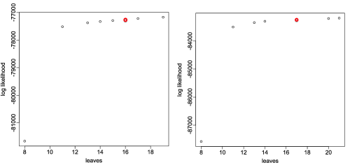
Figure 1: Log-likelihood corresponding to the champion trees for BP and EP according to the number of leaves.

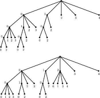
Figure 2: Champion trees for BP (left) and EP (right).

Besides discriminating EP and BP, the selected trees have properties which are linguistically interpretable. First, 4 is a context or the ending symbol of a context, not only in the two selected trees, but actually in all the champion trees. This is a welcome result on linguistic grounds since it is reasonable to think that the successive sentences in a text are rhythmically, as well as syntactically, independent.

Second, in both trees, nonstressed internal syllables provide poor information about the future. Three successive symbols zero are needed to constitute a context. This is consistent with linguistic common beliefs according to which nonstressed noninitial syllables do not play a salient role in rhythm by their own, but only as parts of bigger rhythmic units like phonological words.

Note that a stressed syllable alone is not enough to predict the next symbol either. The tables of transition probabilities (Table 9) show that in both languages the distribution of what follows a stressed syllable is dependent on the presence or absence of a preceding phonological word boundary in the two preceding steps. This fact, arguably derivable from the morphology of Portuguese, does not discriminate EP and BP. By morphology, we mean the way words of a particular language are constituted. This is not surprising since to a great extent EP and BP share the same lexicon.

Finally, according to the selected trees, the main difference between the two languages is that whereas in BP both 2 (unstressed boundary of a phonological word) and 3 (stressed boundary of a phonological word) are contexts, in EP only 3 is a context. This means that in EP, as far as noninitial stress words are concerned, the choice of lexical items is dependent on the rhythmic properties of the preceding words. This is not true when the word begins with a stressed syllable. This does not occur in BP, where word boundaries are always contexts, and as such insensitive to what occurs before, independently of being stressed or not.

Table 9: Probabilistic context tree for BP (left) and EP (right)

BP					EP
$\bolds{w}$	$\bolds{p(0|w)}$	$\bolds{p(1|w)}$	$\bolds{p(2|w)}$	$\bolds{p(3|w)}$	$\bolds{w}$	$\bolds{p(0|w)}$	$\bolds{p(1|w)}$	$\bolds{p(2|w)}$	$\bolds{p(3|w)}$
0000	0.28	0.72	0.00	$0.00$	000	0.27	0.73	0.00	0.00
2000	0.32	0.68	0.00	$0.00$	100	0.00	0.00	0.67	0.25
100	0.00	0.00	0.67	$0.21$	200	0.36	0.64	0.00	0.00
200	0.40	0.60	0.00	$0.00$	300	0.00	0.00	0.70	0.20
300	0.00	0.00	0.67	$0.22$	010	0.05	0.00	0.67	0.19
0010	0.03	0.00	0.67	$0.20$	210	0.08	0.00	0.63	0.22
2010	0.07	0.00	0.66	$0.198$	20	0.45	0.55	0.00	0.00
210	0.08	0.00	0.63	$0.22$	30	0.05	0.00	0.64	0.27
20	0.45	0.55	0.00	$0.00$	001	0.61	0.00	0.28	0.07
30	0.07	0.00	0.64	$0.25$	201	0.72	0.00	0.19	0.07
001	0.62	0.00	0.27	$0.08$	21	0.72	0.00	0.19	0.07
201	0.72	0.00	0.19	$0.07$	02	0.59	0.41	0.00	0.00
21	0.73	0.00	0.18	$0.08$	12	0.55	0.45	0.00	0.00
2	0.60	0.40	0.00	$0.00$	32	0.50	0.50	0.00	0.00
3	0.69	0.00	0.21	$0.10$	42	0.52	0.48	0.00	0.00
4	0.00	0.00	0.66	$0.34$	3	0.69	0.00	0.19	0.12
					4	0.00	0.00	0.65	0.35

These statistical findings are compatible with the current discussion in the linguistic literature concerning the different behavior of phonological words in the two languages [cf. Vigário (2003) and Sândalo et al. (2006), among others].

7 Final discussion

In this article we address the question of the existence of linguistic rhythm fingerprints that can be retrieved from written texts. In particular, we address the question of the rhythmic differences between BP and EP. This is done by encoding two samples of BP and EP newspaper texts, according to some basic rhythmic features. We formulate the rhythmic features retrieval problem as a question of statistical model selection in the class of the variable length Markov chains. The fact that context trees can be linguistically interpreted enables us to compare our statistical results with current linguistic conjectures concerning rhythm.

This approach to the problem of linguistic rhythm retrieval is entirely new. New is our way to encode written texts according to its rhythmic properties and new is also the idea of using context tree models to characterize linguistic rhythm. The data set we analyzed was constituted for the purposes of the present study.

New is also the statistic approach we introduced to select a context tree model out from data. In effect, we introduced the smallest maximizer criterion to estimate the context tree of a chain with memory of variable length from a finite sample. The criterion selects a tree in the class of champion trees. This class coincides with the subset of trees obtained, given a sample, by varying the penalizing constant in the BIC criterion. For this reason, the smallest maximizer criterion actually suggests a tuning procedure for VLMC selection using the BIC. Therefore, the present paper is a contribution to the solution of the important problem of constant-free model selection in the class of variable length Markov chains.

To our knowledge, Bühlmann (2000) was the first to address the problem of how to tune a context tree estimator, in the case of the algorithm context. This paper proposes the following tuning procedure. First, use the algorithm context with different values of the threshold to obtain a sequence of candidate trees. For each one of these candidate trees estimate a global risk function, as, for example, the Final Prediction Error (FPE) or the Kullback–Leibler Information (KLI), by using a parametric bootstrap approach. Then choose as cutoff parameter the one providing the tree with smallest estimated risk.

In the above mentioned paper there is no proof that the sequence of nested trees obtained by the pruning procedure using the algorithm context will contain eventually almost surely the tree generating the sample, which in our case is given in Theorem 6. It also misses the crucial point of the change of regime in the set of champion trees, which is given in our Theorem 7.

The change of regime was not missed by the more recent paper of Dalevi and Dubhashi (2005). They extend to chains with memory of variable length the order estimator introduced in Peres and Shields (2005). They suggest without any rigorous proof that at the correct order there exists a sharp transition that can be identified from a finite sample. Then they apply the criterion to the identification of sequence similarity in DNA. Our main contribution with respect to this paper is the rigorous proof of Theorem 8, as well as the algorithm implementing the smallest maximizer criterion.

From an applied statistics point of view, in our simulation study the Peres–Shields criterion had a very poor performance when compared to the BIC and SMC procedures. This suggests that the Peres–Shields estimator requires bigger sample sizes to be effective, at least in the case of VLMCs.

Modeling linguistic data as a stochastic process is by no means a new idea. Actually this was the original motivation of Markov himself when he introduced his famous chains at the beginning of the 20th century. Even the more specific question of linguistic rhythm was already addressed in the statistic literature, in particular, by Kolmogorov who looked for statistical regularities discriminating poems from different Russian authors [see, e.g., Kolmogorov and Rychkova (1999)]. However, the issue of the existence of different rhythmic classes of languages, as well as the question of the existence of rhythmic fingerprints in written texts and their retrieval, is still largely open.

The approach proposed here offers a new perspective to the domain of linguistic rhythm. It also proposes a concrete statistical tool to identify rhythmic features in written texts. But the interest of our approach goes far beyond its linguistic original motivation. The smallest maximizer criterion and the algorithm implementing it have a broad application in statistical data analysis and constitute an effective contribution to the question of constant free model selection with large but finite samples.

Appendix A Mathematical proofs

We begin this section by presenting the algorithm to compute the BIC context tree estimator $\hat{\tau}_{\mathrm{BIC}}(X_{1}^{n};c)$ for any given constant $c>0$.

For a string $w$ with $\ell(w)\leq d$ and $\sum_{a\in A}N_{n}(wb)>0$ define

$$L_{w}(X_{1}^{n})=\prod_{a\in A}\hat{p}_{n}(a|w)^{N_{n}(wa)}$$

and $\operatorname{df}(w)=\sum_{a\in A}\chi(wa)$. Then, for any constant $c>0$ define recursively the value

$$V_{w}^{c}(X_{1}^{n})=\cases{\displaystyle\max\biggl{\{}n^{-c\cdot\operatorname{df}(w)}L_{w}(X_{1}^{n}),\prod_{a\in A}V^{c}_{aw}(X_{1}^{n})\biggr{\}},&\quad if $0\leq\ell(w)<d$,\vspace*{2pt}\cr n^{-c\cdot\operatorname{df}(w)}L_{w}(X_{1}^{n}),&\quad if $\ell(w)=d$,}$$

and the indicator

$$\delta_{w}^{c}(X_{1}^{n})=\cases{1,&\quad if $0\leq\ell(w)<d$ and $\displaystyle\prod_{a\in A}V^{c}_{aw}(X_{1}^{n})>n^{-c\cdot\operatorname{df}(w)}L_{w}(X_{1}^{n})$,\vspace*{2pt}\cr 0,&\quad if $0\leq\ell(w)<d$ and $\displaystyle\prod_{a\in A}V^{c}_{aw}(X_{1}^{n})\leq n^{-c\cdot\operatorname{df}(w)}L_{w}(X_{1}^{n})$,\vspace*{2pt}\cr 0,&\quad if $\ell(w)=d$.}$$

Now, for any finite string $w$, with $\ell(w)\leq d$ and for any tree $\tau\in\mathcal{T}_{n}$, we define the irreducible tree $\tau_{w}$ as the set of branches in $\tau$ which have $w$ as a suffix, that is,

$$\tau_{w}=\{u\in\tau\dvtx w\preceq u\}.$$

Let $\mathcal{T}_{w}(X_{1}^{n})$ be the set of all trees defined in this way, that is,

$$\mathcal{T}_{w}(X_{1}^{n})=\{\tau_{w}\dvtx\tau\in\mathcal{T}_{n}\}.$$

If $w$ is a sequence such that $\delta_{w}^{c}(X_{1}^{n})=1$, we define the maximizing tree assigned to the sequence $w$ as the tree $\tau_{w}^{M}(X_{1}^{n})\in\mathcal{T}_{w}(X_{1}^{m})$ given by

$$\tau_{w}^{M}(X_{1}^{n})=\{u\dvtx\delta_{u}^{c}(X_{1}^{n})=0,\delta_{v}^{c}(X_{1}^{n})=1\mbox{ for all }w\preceq v\prec u\}.$$

On the other hand, if $\delta_{w}^{c}(X_{1}^{n})=0$, we define $\tau_{w}^{M}(X_{1}^{n})=\{w\}$.

The following lemma, proven in Csiszár and Talata (2006), is the key for the efficient computation of the BIC context tree estimator. We omit its proof here.

Lemma 9

For any finite string $w$, with $\ell(w)\leq d$, we have

$$V_{w}^{c}(X_{1}^{n})=\max_{\tau\in T_{w}(X_{1}^{n})}\prod_{u\in\tau}n^{-c\cdot\operatorname{df}(u)}L_{u}(X_{1}^{n})=\prod_{u\in\tau_{w}^{M}(X_{1}^{n})}n^{-c\cdot\operatorname{df}(u)}L_{u}(X_{1}^{n}).$$ (6)

The second equality in (6) implies, in particular, that

$$\hat{\tau}_{\mathrm{BIC}}(X_{1}^{n})=\tau_{\lambda}^{M}(X_{1}^{n})=\{u\dvtx\delta_{u}^{c}(X_{1}^{n})=0,\delta_{v}^{c}(X_{1}^{n})=1\mbox{ for all }v\prec u\}$$

and the BIC context tree estimator can be obtained by computing the functions $V_{w}^{c}(X_{1}^{n})$ and $\delta_{w}^{c}(X_{1}^{n})$ over the set of sequences $w$ satisfying $\ell(w)\leq d$ and $\sum_{a\in A}N_{n}(wb)>0$.

Proof of Theorem 6

First recall that the BIC context tree estimator is strongly consistent for any constant $c>0$. Therefore, since the set $\mathcal{C}$ is countable, it follows that eventually almost surely $\tau^{*}\in\mathcal{C}_{n}$ as $n\rightarrow\infty$.

The fact that the champion trees are ordered by $\prec$ follows immediately from the following lemma.

Lemma 10

Let $0<c_{1}<c_{2}$ be arbitrary positive constants. Then

$$\hat{\tau}_{\mathrm{BIC}}(X_{1}^{n};c_{1})\succeq\hat{\tau}_{\mathrm{BIC}}(X_{1}^{n};c_{2}).$$

Denote by $\tau^{1}=\hat{\tau}_{\mathrm{BIC}}(X_{1}^{n};c_{1})$ and $\tau^{2}=\hat{\tau}_{\mathrm{BIC}}(X_{1}^{n};c_{2})$. Suppose that it is not true that $\tau^{1}\succeq\tau^{2}$. Then there exists a sequence $w\in\tau^{1}$ and $w^{\prime}\in\tau^{2}$ such that $w$ is a proper suffix of $w^{\prime}$. This implies that $\tau^{2}_{w}\neq\varnothing$. Since $\tau^{2}$ is irreducible, we have that $|\tau^{2}_{w}|\geq 2$. Then, using the definition of maximizing tree, we obtain

$$\log L_{w}(X_{1}^{n}) \geq \sum_{w^{\prime}\in\tau^{2}_{w}}\log L_{w^{\prime}}(X_{1}^{n})+c_{1}\biggl{(}\operatorname{df}(w)-\sum_{w^{\prime}\in\tau^{2}_{w}}\operatorname{df}(w^{\prime})\biggr{)}\log n$$

$$\geq \sum_{w^{\prime}\in\tau^{2}_{w}}\log L_{w^{\prime}}(X_{1}^{n})+c_{2}\biggl{(}\operatorname{df}(w)-\sum_{w^{\prime}\in\tau^{2}_{w}}\operatorname{df}(w^{\prime})\biggr{)}\log n$$

$$> \log L_{w}(X_{1}^{n}),$$

which is a contradiction. The first inequality follows from the assumption that $\tau^{1}=\hat{\tau}_{\mathrm{BIC}}(X_{1}^{n};c_{1})$ and the second equality in (6). To derive the second inequality, we use the fact that $0<c_{1}<c_{2}$ and $\operatorname{df}(w)-\sum_{w^{\prime}\in\tau^{2}_{w}}\operatorname{df}(w^{\prime})<0$. Finally, the last inequality leading to the contradiction follows from $\tau^{2}=\hat{\tau}_{\mathrm{BIC}}(X_{1}^{n};c_{2})$ and again the second equality in (6). We conclude that $\tau^{1}\succeq\tau^{2}$.

Proof of Theorem 7

To prove (1) let $\tau\in\mathcal{C}_{n}$ be such that $\tau\prec\tau^{*}$. Then

$$\log L_{\tau}(X_{1}^{n})-\log L_{\tau^{*}}(X_{1}^{n})$$

$$\qquad=\sum_{w^{\prime}\in\tau,a\in A}N_{n}(w^{\prime}a)\log\hat{p}_{n}(a|w^{\prime})-\sum_{w\in\tau^{*},a\in A}N_{n}(wa)\log\hat{p}_{n}(a|w)$$

$$\qquad=\sum_{w^{\prime}\in\tau}\sum_{w\in\tau^{*},w\succ w^{\prime}}\sum_{a\in A}N_{n}(wa)\log\frac{\hat{p}_{n}(a|w^{\prime})}{\hat{p}_{n}(a|w)}.$$

Dividing by $n$ and using Jensen’s inequality in the right-hand side, we have that

$$\sum_{w^{\prime}\in\tau}\sum_{w\in\tau^{*},w\succ w^{\prime}}\sum_{a\in A}\frac{N_{n}(wa)}{n}\log\frac{\hat{p}_{n}(a|w^{\prime})}{\hat{p}_{n}(a|w)}$$

$$\qquad\longrightarrow\sum_{w^{\prime}\in\tau^{\prime}}\sum_{w\in\tau^{*},w\succ w^{\prime}}\sum_{a\in A}p^{*}(wa)\log\frac{p^{*}(a|w^{\prime})}{p^{*}(a|w)}<0$$

as $n$ goes to $+\infty$ (by the minimality of $\tau^{*}$). Then, for a sufficiently large $n$ there exists a constant $c(\tau^{*},\tau)>0$ such that

$$\log L_{\tau^{*}}(X_{1}^{n})-\log L_{\tau}(X_{1}^{n})\geq c(\tau^{*},\tau)n.$$

To prove (2), we have that

$$\log L_{\tau^{\prime}}(X_{1}^{n})-\log L_{\tau}(X_{1}^{n})$$

$$\qquad=\sum_{w^{\prime}\in\tau^{\prime},a\in A}N_{n}(w^{\prime}a)\log\hat{p}_{n}(a|w^{\prime})-\sum_{w\in\tau,a\in A}N_{n}(wa)\log\hat{p}_{n}(a|w)$$

$$\qquad\leq\sum_{w^{\prime}\in\tau^{\prime},a\in A}N_{n}(w^{\prime}a)\log\hat{p}_{n}(a|w^{\prime})-\sum_{w\in\tau,a\in A}N_{n}(wa)\log p^{*}(a|w)$$

$$\qquad=\sum_{w\in\tau}\sum_{w^{\prime}\in\tau^{\prime},w^{\prime}\succ w}\sum_{a\in A}N_{n}(w^{\prime}a)\log\frac{\hat{p}_{n}(a|w^{\prime})}{p^{*}(a|w)}$$

$$\qquad=\sum_{w\in\tau}\sum_{w^{\prime}\in\tau^{\prime},w^{\prime}\succ w}N_{n}(w^{\prime}\cdot)D(\hat{p}_{n}(\cdot|w^{\prime})\|p^{*}(\cdot|w)).$$

By Lemmas 6.2 and 6.3 in Csiszár and Talata (2006) we have that, if $n$ is sufficiently large, we can bound above the last term by

$$\sum_{w\in\tau}\sum_{w^{\prime}\in\tau^{\prime},w^{\prime}\succ w}N_{n}(w^{\prime}\cdot)\sum_{a\in A}\frac{[\hat{p}_{n}(a|w^{\prime})-p^{*}(a|w)]^{2}}{p^{*}(a|w)}$$

$$\qquad\leq\sum_{w\in\tau}\sum_{w^{\prime}\in\tau^{\prime},w^{\prime}\succ w}N_{n}(w^{\prime}\cdot)\frac{1}{p^{*}_{\min}}|A|\frac{\delta\log n}{N_{n}(w^{\prime}\cdot)},$$

where $p_{\min}^{*}=\min_{w\in\tau,a\in A}\{p^{*}(a|w)\dvtx p^{*}(a|w)>0\}$. This concludes the proof of Theorem 7.

Proof of Theorem 8

It follows directly from Theorems 6 and 7.

Appendix B Description of the encoded samples

The newspaper articles of the sample were selected in the following way. We first randomly selected 20 editions for each newspaper for each year. Inside each edition we discarded all the texts with less than 1,000 words as well as some type of articles (interviews, synopsis, transcriptions of laws and collected works) which are unsuitable for our purposes. From the remaining articles we randomly selected one article for each previously selected edition.

Before encoding each one of the selected texts, they were submitted to a linguistically oriented cleaning procedure. Hyphenated compound words were rewritten as two separate words, except when one of the components is unstressed. Suspension points, question marks and exclamation points were replaced by periods. Dates and special symbols like “%” were spelled out as words. All parentheses were removed.

To use the smallest maximizer criterion, we need to compute the number of degrees of freedom of each candidate context tree. To do this, we must take into account the linguistic restrictions on the symbolic chain obtained after encoding. The restrictions are the following: [(1)]

Due to Portuguese morphological constraints, a stressed syllable (encoded by 1 or 3) can be immediately followed by at most three unstressed syllables (encoded by 0).

Since by definition any phonological word must contain one and only one stressed syllable (encoded by 1 or 3), after a symbol 3 no symbol 1 is allowed, before a symbol 2 (nonstressed syllable starting a phonological word) appears.

By the same reason, after a symbol 2 no symbols 2 or 3 are allowed before a symbol 1 appears.

As sentences are formed by the concatenation of phonological words, the only symbols allowed after 4 (end of sentence) are the symbols 2 or 3 (beginning of phonological word).

References

- Abercrombie (1967) {bbook}[auto:STB—2011/12/05—07:51:37] \bauthor\bsnmAbercrombie, \bfnmD.\binitsD. (\byear1967). \btitleElements of General Phonetics. \bpublisherAldine, \baddressChicago. \bptokimsref \endbibitem
- Bühlmann (2000) {barticle}[mr] \bauthor\bsnmBühlmann, \bfnmPeter\binitsP. (\byear2000). \btitleModel selection for variable length Markov chains and tuning the context algorithm. \bjournalAnn. Inst. Statist. Math. \bvolume52 \bpages287–315. \biddoi=10.1023/A:1004165822461, issn=0020-3157, mr=1763564 \bptokimsref \endbibitem
- Bühlmann and Wyner (1999) {barticle}[mr] \bauthor\bsnmBühlmann, \bfnmPeter\binitsP. and \bauthor\bsnmWyner, \bfnmAbraham J.\binitsA. J. (\byear1999). \btitleVariable length Markov chains. \bjournalAnn. Statist. \bvolume27 \bpages480–513. \biddoi=10.1214/aos/1018031204, issn=0090-5364, mr=1714720 \bptokimsref \endbibitem
- Csiszár and Talata (2006) {barticle}[mr] \bauthor\bsnmCsiszár, \bfnmImre\binitsI. and \bauthor\bsnmTalata, \bfnmZsolt\binitsZ. (\byear2006). \btitleContext tree estimation for not necessarily finite memory processes, via BIC and MDL. \bjournalIEEE Trans. Inform. Theory \bvolume52 \bpages1007–1016. \biddoi=10.1109/TIT.2005.864431, issn=0018-9448, mr=2238067 \bptokimsref \endbibitem
- Cuesta-Albertos et al. (2007) {barticle}[mr] \bauthor\bsnmCuesta-Albertos, \bfnmJuan Antonio\binitsJ. A., \bauthor\bsnmFraiman, \bfnmRicardo\binitsR., \bauthor\bsnmGalves, \bfnmAntonio\binitsA., \bauthor\bsnmGarcia, \bfnmJesús\binitsJ. and \bauthor\bsnmSvarc, \bfnmMarcela\binitsM. (\byear2007). \btitleIdentifying rhythmic classes of languages using their sonority: A Kolmogorov–Smirnov approach. \bjournalJ. Appl. Stat. \bvolume34 \bpages749–761. \bptokimsref \endbibitem
- Dalevi and Dubhashi (2005) {bincollection}[mr] \bauthor\bsnmDalevi, \bfnmDaniel\binitsD. and \bauthor\bsnmDubhashi, \bfnmDevdatt\binitsD. (\byear2005). \btitleThe Peres–Shields order estimator for fixed and variable length Markov models with applications to DNA sequence similarity. In \bbooktitleAlgorithms in Bioinformatics. \bseriesLecture Notes in Computer Science \bvolume3692 \bpages291–302. \bpublisherSpringer, \baddressBerlin. \biddoi=10.1007/11557067_24, mr=2226840 \bptokimsref \endbibitem
- Dauer (1983) {barticle}[auto:STB—2011/12/05—07:51:37] \bauthor\bsnmDauer, \bfnmR.\binitsR. (\byear1983). \btitleStress-timing and syllable-timing reanalized. \bjournalJournal of Phonetics \bvolume11 \bpages51–62. \bptokimsref \endbibitem
- de Carvalho (1988) {barticle}[auto:STB—2011/12/05—07:51:37] \bauthor\bparticlede \bsnmCarvalho, \bfnmBrandão J.\binitsB. J. (\byear1988). \btitleRéduction vocalique, quantité et accentuation: Pour une explication structurale de la divergence entre portugais lusitanien et portugais brésilien. \bjournalBoletim de Filologia \bvolume32 \bpages5–26. \bptokimsref \endbibitem
- Efron and Tibshirani (1993) {bbook}[mr] \bauthor\bsnmEfron, \bfnmBradley\binitsB. and \bauthor\bsnmTibshirani, \bfnmRobert J.\binitsR. J. (\byear1993). \btitleAn Introduction to the Bootstrap. \bseriesMonographs on Statistics and Applied Probability \bvolume57. \bpublisherChapman & Hall, \baddressNew York. \bidmr=1270903 \bptokimsref \endbibitem
- Frota and Vigário (2001) {barticle}[auto:STB—2011/12/05—07:51:37] \bauthor\bsnmFrota, \bfnmS.\binitsS. and \bauthor\bsnmVigário, \bfnmM.\binitsM. (\byear2001). \btitleOn the correlates of rhythm distinctions: The European/Brazilian Portuguese case. \bjournalProbus \bvolume13 \bpages247–275. \bptokimsref \endbibitem
- Galves and Leonardi (2008) {bincollection}[mr] \bauthor\bsnmGalves, \bfnmAntonio\binitsA. and \bauthor\bsnmLeonardi, \bfnmFlorencia\binitsF. (\byear2008). \btitleExponential inequalities for empirical unbounded context trees. In \bbooktitleIn and Out of Equilibrium. 2. \bseriesProgress in Probability \bvolume60 \bpages257–269. \bpublisherBirkhäuser, \baddressBasel. \biddoi=10.1007/978-3-7643-8786-0_12, mr=2477385 \bptokimsref \endbibitem
- Galves and Löcherbach (2008) {bmisc}[auto:STB—2011/12/05—07:51:37] \bauthor\bsnmGalves, \bfnmA.\binitsA. and \bauthor\bsnmLöcherbach, \bfnmE.\binitsE. (\byear2008). \bhowpublishedStochastic chains with memory of variable length. In Festchrift in Honour of Jorma Rissanen on the Occasion of His 70th Birthday (Grünwald et al., eds.). TICSP Series 38 117–133. Tampere Univ. Technology, Tampere, Finland. \bptokimsref \endbibitem
- Galves et al. (2011) {bmisc}[auto:STB—2011/12/05—07:51:37] \bauthor\bsnmGalves, \bfnmA.\binitsA., \bauthor\bsnmGalves, \bfnmC.\binitsC., \bauthor\bsnmGarcia, \bfnmJ. E.\binitsJ. E., \bauthor\bsnmGarcia, \bfnmN. L.\binitsN. L. and \bauthor\bsnmLeonardi, \bfnmF.\binitsF. (\byear2011). \bhowpublishedSupplement to “Context tree selection and linguistic rhythm retrieval from written texts.” DOI:10.1214/11-AOAS511SUPP. \bptokimsref \endbibitem
- Garivier (2006) {bmisc}[auto:STB—2011/12/05—07:51:37] \bauthor\bsnmGarivier, \bfnmA.\binitsA. (\byear2006). \bhowpublishedModèles contextuels et alphabets infinis en théorie de l’information. Ph.D. thesis, Univ. Paris Sud. \bptokimsref \endbibitem
- Kleinhenz (1997) {bmisc}[auto:STB—2011/12/05—07:51:37] \bauthor\bsnmKleinhenz, \bfnmU.\binitsU. (\byear1997). \bhowpublishedDomain typology at the phonology-syntax interface. In Interfaces in Linguistic Theory (G. Matos et al., eds.) 201–220. APL/Colibri, Lisboa. \bptokimsref \endbibitem
- Kolmogorov and Rychkova (1999) {barticle}[mr] \bauthor\bsnmKolmogorov, \bfnmA. N.\binitsA. N. and \bauthor\bsnmRychkova, \bfnmN. G.\binitsN. G. (\byear2000). \btitleAnalysis of russian verse rhythm, and probability theory. \bjournalTheory Probab. Appl. \bvolume44 \bpages375–385. \bptnotecheck year\bptokimsref \endbibitem
- Lloyd (1940) {bmisc}[auto:STB—2011/12/05—07:51:37] \bauthor\bsnmLloyd, \bfnmJ.\binitsJ. (\byear1940). \bhowpublishedSpeech Signals in Telephony. Pitman, London. \bptokimsref \endbibitem
- Mehler et al. (1996) {bincollection}[auto:STB—2011/12/05—07:51:37] \bauthor\bsnmMehler, \bfnmJ.\binitsJ., \bauthor\bsnmDupoux, \bfnmE.\binitsE., \bauthor\bsnmNazzi, \bfnmT.\binitsT. and \bauthor\bsnmDehaene-Lambertz, \bfnmG.\binitsG. (\byear1996). \btitleCoping with linguistic diversity: The Infant’s viewpoint. In \bbooktitleSignal to Syntax: Bootstrapping from Speech to Grammar in Early Acquisition (\beditor\bfnmJ.\binitsJ. \bsnmMorgan and \beditor\bfnmK.\binitsK. \bsnmDemuth, eds.) \bpages101–116. \bpublisherLEA, \baddressHillsdale, NJ. \bptokimsref \endbibitem
- Nespor and Vogel (1986) {bbook}[auto:STB—2011/12/05—07:51:37] \bauthor\bsnmNespor, \bfnmM.\binitsM. and \bauthor\bsnmVogel, \bfnmI.\binitsI. (\byear1986). \btitleProsodic Phonology. \bpublisherForis, \baddressDordrecht. \bptokimsref \endbibitem
- Peres and Shields (2005) {bmisc}[auto:STB—2011/12/05—07:51:37] \bauthor\bsnmPeres, \bfnmY.\binitsY. and \bauthor\bsnmShields, \bfnmP.\binitsP. (\byear2005). \bhowpublishedTwo new Markov order estimators. Unpublished manuscript. Available at arXiv:math/0506080v1. \bptokimsref \endbibitem
- Pike (1945) {bbook}[auto:STB—2011/12/05—07:51:37] \bauthor\bsnmPike, \bfnmK. L.\binitsK. L. (\byear1945). \btitleThe Intonation of American English. \bpublisherUniversity of Michigan Press, \baddressAnn Arbor. \bptokimsref \endbibitem
- Ramus (2002) {bincollection}[auto:STB—2011/12/05—07:51:37] \bauthor\bsnmRamus, \bfnmF.\binitsF. (\byear2002). \btitleAcoustic correlates of linguistic rhythm: Perspectives. In \bbooktitleProc. First International Conference on Speech Prosody (\beditorB. Bel and \beditorI. Marlien, eds.) \bpages323–326. \bpublisherLaboratoire Parole et Langage, \baddressAix-en-Provence. \bptokimsref \endbibitem
- Ramus, Nespor and Mehler (1999) {barticle}[auto:STB—2011/12/05—07:51:37] \bauthor\bsnmRamus, \bfnmF.\binitsF., \bauthor\bsnmNespor, \bfnmM.\binitsM. and \bauthor\bsnmMehler, \bfnmJ.\binitsJ. (\byear1999). \btitleCorrelates of linguistic rhythm in the speech signal. \bjournalCognition \bvolume73 \bpages265–292. \bptokimsref \endbibitem
- Rissanen (1983) {barticle}[mr] \bauthor\bsnmRissanen, \bfnmJorma\binitsJ. (\byear1983). \btitleA universal data compression system. \bjournalIEEE Trans. Inform. Theory \bvolume29 \bpages656–664. \biddoi=10.1109/TIT.1983.1056741, issn=0018-9448, mr=0730903 \bptokimsref \endbibitem
- Ron, Singer and Tishby (1996) {barticle}[auto:STB—2011/12/05—07:51:37] \bauthor\bsnmRon, \bfnmD.\binitsD., \bauthor\bsnmSinger, \bfnmY.\binitsY. and \bauthor\bsnmTishby, \bfnmN.\binitsN. (\byear1996). \btitleThe power of amnesia: Learning probabilistic automata with variable memory length. \bjournalMachine Learning \bvolume25 \bpages117–149. \bptokimsref \endbibitem
- Sândalo et al. (2006) {barticle}[auto:STB—2011/12/05—07:51:37] \bauthor\bsnmSândalo, \bfnmF.\binitsF., \bauthor\bsnmAbaurre, \bfnmM. B.\binitsM. B., \bauthor\bsnmMandel, \bfnmA.\binitsA. and \bauthor\bsnmGalves, \bfnmC.\binitsC. (\byear2006). \btitleSecondary stress in two varieties of portuguese and the sotaq optimality based computer program. \bjournalProbus \bvolume18 \bpages97–125. \bptokimsref \endbibitem
- Vigário (2003) {bbook}[auto:STB—2011/12/05—07:51:37] \bauthor\bsnmVigário, \bfnmM.\binitsM. (\byear2003). \btitleThe Prosodic Word in European Portuguese. \bpublisherde Gruyter, \baddressBerlin. \bptokimsref \endbibitem
- Willems, Shtarkov and Tjalkens (1995) {barticle}[auto:STB—2011/12/05—07:51:37] \bauthor\bsnmWillems, \bfnmF. M. J.\binitsF. M. J., \bauthor\bsnmShtarkov, \bfnmY. M.\binitsY. M. and \bauthor\bsnmTjalkens, \bfnmT. J.\binitsT. J. (\byear1995). \btitleThe context-tree weighting method: Basic properties. \bjournalIEEE Trans. Inform. Theory \bvolume41 \bpages653–664. \bptokimsref \endbibitem