Techniques to study cosmic ray anisotropies

Abstract

These lectures review some of the techniques used to analyse the arrival direction distribution of Cosmic Rays, and some relevant results on the field.

1 Introduction

The study of the anisotropies in the arrival directions of cosmic rays (CR) provides a handle, together with the spectrum and composition studies, to face several open questions in the field like: which are the sources of cosmic rays?, how do CRs propagate?, which is the CR composition?, how are the galactic and extragalactic magnetic fields?

The cosmic ray flux has proven to be very close to isotropic and thus very careful studies are needed to measure the anisotropies. Before entering the discussion of the techniques used, which are the main scope of these lectures, we will review some topics that are relevant to understand the kind of anisotropies that can be expected in different energy ranges. These are: the matter distribution in our neighbourhood, the galactic and extragalactic magnetic field effects on the CR propagation (deflections, flux amplification, multiple images) and the Greisen Zatsepin Kuzmin (GZK) horizon.

1.1 Our local universe

The distribution of matter around us is not isotropic. The Milky Way is a spiral galaxy. The disk, that has a width of about 1 kpc (1 pc $\sim$ 3 ly), contains in the spiral arms most of the visible stars, as well as atomic gas with a density of approximately one particle per cm³. The solar system is located at 8.5 kpc from the galactic center. A regular magnetic field component permeates the disk. The Galaxy is also permeated by a turbulent magnetic field where charged cosmic ray particles are trapped and that probably extends few kpc outside the disk. The Galaxy has also a spheroid (or stellar halo) of more spherical shape constituted by an older stellar population and a smaller amount of gas (with density $\sim 0.01/$cm³), that extends up to a distance of about 15 kpc. It has a central bulge with a bar-like shape. A larger dark matter halo is also present, which existence is evidenced by its gravitational effects, such as the rotation curves of stars and gas that remain flat up to distances larger than those containing the visible matter, but its composition is not yet known. The Galaxy has also a massive black hole in the center with a mass of few $10^{6}$M_⊙ .

The Milky Way and its neighbour galaxy Andromeda are the most prominent members of a small cluster of about 30 galaxies called the Local Group, with a diameter of about 2 Mpc.

The Local Group forms part of the Local Supercluster, a large agglomerate of about 100 galaxy clusters and groups, that is dominated by the Virgo cluster located near its center (distant about 18 Mpc from the Milky Way). Virgo is a large cluster, with more than 2000 galaxies, including the prominent radio galaxy M87.

At even larger scales the distribution of clusters shows an inhomogeneous distribution with large filaments and voids. Only at scales larger than few hundred Mpc the universe starts to look homogeneous.

1.2 Magnetic field effects on the CR propagation

The galactic magnetic field has a regular and a turbulent component. Despite a considerable observational effort, both are still poorly known han ; beck . From the observation of polarized radio emission of other face-on spiral galaxies it is known that the regular magnetic field follows the spiral pattern of the stars distribution, while radio polarization measurements in edge-on galaxies show the existence of magnetic halos extending few kpc above and below the galactic disks.

In our own Galaxy, Faraday rotation measures of pulsars and extragalactic radio sources indicate that the regular magnetic field follows the spiral pattern in the disk, with a local value $B_{reg}\simeq 2-3\ \mu$G. han . The turbulent field is thought to be larger in rms amplitude than the regular one, with a coherence length of approximately 100 pc.

The propagation of charged CRs is affected by the magnetic fields (both galactic and extragalactic) present along their trajectories. The deflection of ultra-relativistic charged particles is proportional to their charges and inversely proportional to their energy

$\vec{F}=m\gamma\dot{\vec{v}}={q\over c}\vec{v}\times\vec{B},\ \ \ \ \ \ \ \ \vec{v}=c\hat{u}.$

Then, the direction of propagation is given by

$\hat{u}=\hat{u}_{0}+{Ze\over E}\int dl\ \hat{u}\times\vec{B}.$

A CR of charge $Ze$ and energy $E$ in a constant field $B$ describes a circle of Larmor radius

$r_{L}\simeq{{E/Z}\over{10^{15}eV}}{{\mu G}\over B}pc.$

Then, for $E/Z<10^{18}$ eV ($\equiv$ 1 EeV) cosmic ray trajectories wind around the magnetic field lines and they remain confined by the galactic magnetic field for a long time, while for larger energies their trajectories are only moderately perturbed and they are not confined in the Galaxy. For $E/Z<10^{17}$ eV they scatter off the turbulent magnetic field irregularities, that have a coherence scale $l\leq r_{L}$, make a random walk and diffuse.

Liouville theorem

An isotropic flux of CRs remains isotropic after propagating through a magnetic field. According to the Liouville theorem the phase space distribution $f(\vec{r},\vec{p})$ is constant along cosmic ray trajectories if there are no processes that dis troy or create particles. The intensity of CRs, defined as the number of particles crossing a unit area $dA$ per unit time $dt$ and unit solid angle $d\Omega$ with energy within $E$ and $E+dE$ is given by $I=dN/(dAdtd\Omega dE)$ and we can write $dN=f(\vec{r},\vec{p})d^{3}rd^{3}p$, with $d^{3}r=dAvdt$ and $d^{3}p=p^{2}dpd\Omega$. Then $I=f(\vec{r},\vec{p})vp^{2}dp/dE=f(\vec{r},\vec{p})p^{2}$. Since $p$ is constant along the trajectory, $I$ is also constant. As a consequence, an isotropic CR flux remains isotropic unless there is a ’shadowing effect’, i.e. there exist directions from which particles cannot reach the detector coming from infinity. For example at low energies this happens because of the Earth ‘shadow’: trajectories of antiparticles leaving from the detector hit the Earth due to the deflections in the geomagnetic field. This in particular gives rise to the so-called East-West effect: Protons with energy smaller than few GeV are not able to reach the Earth from the east. The sign of this E-W asymmetry was used to infer that CR primaries are positively charged. Towards the poles the threshold is smaller and this has the effect of increasing the CR intensity with latitude at low energies (’latitude effect’).

Deflection of charged particles in the Galactic magnetic field

As we have discussed the deflection of charged particles is inversely proportional to their energy, and only for $E/Z\gg 10^{19}eV$ the deflections in the Galactic magnetic field are expected to become smaller than a few degrees and CR astronomy could become feasible. If the Galactic $B$ field (and composition) were known, one could correct the arrival direction to search for the source. This could be done by ‘backtracking antiparticles’ leaving the detector with the reverse velocity of the incoming CR. According to the Liouville theorem the magnetic fields cannot produce anisotropies in an isotropic flux, but they do in fact affect anisotropic fluxes in different ways: the flux can be amplified in some regions and deamplified in others in an energy dependent way, and even multiple images of sources located in some regions can appear. These effects can be visualized plotting for a regular grid of arrival directions at Earth the corresponding directions from which the particles arrived to the galactic halo. This is shown in Figure 1 for a particular model of the regular magnetic field and for particles with $E/Z$ = 20 EeV. One may picture this distorted image of the sky seen from the Earth as a sheet (the ‘sky sheet’) that can be stretched and folded. A source located in a fold of this sky sheet will have multiple images, i.e. cosmic rays of the same energy can arrive to the Earth from several different directions. Moreover, the flux coming from a source in a region where the sheet is stretched will appear demagnified while that from a source in a compressed region will appear magnified toes .

Figure 1: ’Sky sheet’ in galactic coordinates.

If several CRs with different energies coming from one source are detected it would be possible to measure the integrated perpendicular component of the magnetic field along the CR trajectory and locate the actual source position.

Magnetic lensing phenomena also appear for turbulent fields turb . The deflections in a turbulent field can be viewed as a random walk of the CR particles that suffer in each field domain a deflection in a random direction. The accumulated deflection after traversing a distance $L$ in a field with coherence length $L_{c}$ is given by

$\delta_{rms}=\sqrt{L/L_{c}}(ZeB_{rms}L_{c}/E)$,

where the last factor corresponds to the mean deflection in one domain.

For $B_{rms}\simeq B_{reg}$, deflections in the turbulent field are smaller than those produced by the regular field, but can dominate the magnetic lensing effects. Multiple images appear below a critical energy $E_{c}$, such that typical transverse displacements among different paths become of order the correlation length of the $B$ field ($\delta_{rms}\simeq L_{c}/L$). Typically $E_{c}\simeq 4\times 10^{19}eV\ Z(B_{rms}/5\mu$G$)(L/2$kpc$)^{3/2}(L_{c}/50$pc$)^{-1/2}$. For $E<E_{c}$ , the number of images grows exponentially. A regime is reached with a large number of images, spread over a region of size $\delta_{rms}$ and with mean magnification $\langle A\rangle\simeq 1$ (like twinkling stars).

Magnetic fields are also present outside galaxies, but the observational constraints are still very poor. The amplitude in the central region of clusters may reach the $\mu$G. The distribution is believed to follow the filamentary pattern of the large scale matter distribution. In most of the space it is usually assumed that $B_{rms}=10^{-8}-10^{-9}$ G and the coherence length $L_{c}\sim$Mpc.

1.3 The Greisen-Zatsepin-Kuzmin horizon

Soon after the discovery of the cosmic microwave background (CMB) radiation it was realized by Greisen, Zatsepin and Kuzmin gzk that the fluxes of CR protons with energies of order $10^{20}$ eV and above would be strongly attenuated over distances of a few tens of Mpc. This is due to the energy losses caused by the photo-pion production processes in the interactions of the protons with the CMB photons. Similarly, if CR sources accelerate heavy nuclei, these can photo-disintegrate into lighter ones as they interact with CMB and infrared (IR) photons on their journey to us. In this way the fragments may arrive at the Earth with significantly smaller energies than the parent nuclei produced at the sources. Moreover, both protons and heavy nuclei can further loose energy by pair production processes, although due to the small inelasticities involved the typical attenuation length associated with $e^{+}e^{-}$ production at ultra-high energies is large ($\sim$ 1 Gpc for protons). These processes limit the distance from which ultra-high energy cosmic rays can arrive to the Earth. For example, at energies above $\sim 60$ EeV, cosmic rays should mostly come from nearby sources: in the hypothesis of an homogeneous distribution of sources, $90\%$ of the flux should come from sources closer than $\sim 200$ Mpc and $50\%$ from sources closer than $\sim 100$ Mpc. The distance limits turn out to be similar for iron nuclei (although the responsible processes are different), while lighter nuclei should come from a much closer neighbourhood horizon .

1.3.1 Exposure

For any CR anisotropy analysis it is very important to have a good estimate of the expected flux in any direction for the given experimental setup in the case the CR flux is isotropic. The exposure measures the time integrated effective collecting area in units of km² yr. For each direction of the sky $\omega(\delta,\alpha)$ gives the relative exposure. For a detector in continuous operation it is uniform in right ascension $\alpha$, being only a function of the declination $\delta$.

If the detector is fully efficient for particles arriving with zenith angle $\theta<\theta_{m}$, the exposure has only a $\cos(\theta)$ modulation due to the change in the effective detection area. The zenith of a detector located at latitude $\delta_{0}$ corresponds to a position in the celestial sphere given $\hat{\xi}=(\cos\delta_{0}\cos\alpha_{\xi},\cos\delta_{0}\sin\alpha_{\xi},\sin\delta_{0})$, where $\alpha_{\xi}$ is the right ascension of the detector zenith. A source in a direction $\hat{s}=(\cos\delta_{s}\cos\alpha_{s},\cos\delta_{s}\sin\alpha_{s},\sin\delta_{s})$ is seen at a zenithal angle $\cos\theta=\hat{\xi}\cdot\hat{s}=\cos\delta_{0}\cos\delta_{s}\cos(\alpha_{s}-\alpha_{\xi})+\sin\delta_{0}\sin\delta_{s}$. The exposure towards a direction $\hat{s}$ is proportional to the integral of $\cos\theta(t)$ for all the times when $\theta(t)<\theta_{m}$, and is given by $\omega(\delta)\propto\cos\delta\cos\delta_{0}\sin\alpha_{m}+\alpha_{m}\sin\delta\sin\delta_{0}$, where $\alpha_{m}=\arccos(z)$ (if $-1<z<1$) with $z=(\cos\alpha_{m}-\sin\delta_{0}\sin\delta)/\cos\delta\cos\delta_{0}$, $\alpha_{m}=\pi$ (if $z<-1$) and $\alpha_{m}=0$ (if $z>1$) sommers . The exposure is shown in Figure 2 for a detector at latitude $-35^{\circ}$, corresponding to the Pierre Auger Observatory.

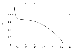
Figure 2: Exposure as a function of declination

Perfect exposure holds for a continuously operating detector at the highest energies where every shower triggers the detector. At lower energies the more inclined showers are more attenuated than the vertical ones and are less effective to trigger the detector, and then the exposure is no longer just proportional to $\cos\theta$. There are two main strategies to compute the exposure in these cases: a semi-analytical method that consists in obtaining the zenith angle distribution from the data itself and then proceed as before with the integration in $\theta(t)$, or the shuffling technique that consists in simulating a large number of fake events using the time and zenith angle distribution of real events from which the isotropic expectation can be obtained.

2 Cosmic ray anisotropies

Different signals of anisotropies are expected to appear at different energies due to the different sources and propagation effects involved that we will briefly discuss here.

At the highest energies the magnetic deflections are expected to be small and the GZK horizon limits the distance from which CR can arrive, then we might expect to observe only events coming from ’nearby’ sources. The expected signals are then: small scale clustering of events coming from the same source, correlation of events with a population of source candidates, intermediate scale clustering reflecting the clustering of local sources. Lowering the energy, the deflections increase and the GZK horizon also increases, then the CR flux is expected to become more isotropic, but we can still expect some intermediate scale clustering and correlation with the sources distribution. Although the distribution is expected to become more isotropic when lowering the energy, the increase in statistics should help to detect the smaller anisotropy signal. At even lower energies, a large scale anisotropy signal coming from the diffusion and drifts of CR in the Galactic magnetic field is expected to be seen.

If there is a neutral component of CRs a point-like signal is expected and a correlation with the source population at the angular resolution scale should appear.

In addition to these intrinsic anisotropies in the CR arrival direction, there is also a large scale anisotropy signal expected from the motion of the detector with respect to the CR rest frame, the so-called Compton Getting effect.

We will now discuss some of the techniques that are used to measure the anisotropies in the CR intensity $I$, that is defined as the number of particles per unit solid angle that pass per unit time through a unit of area perpendicular to the direction of observation $\hat{u}$. The differential (spectral) intensity $I(E)$ is the intensity of particles with energy in the interval from $E$ to $E+dE$.

2.0.1 Large scale anisotropies

The first signal at large angular scales that we look for is a dipole in some direction $\hat{j}$. A dipole gives rise to an intensity $I(\hat{u})=I_{0}+I_{1}\hat{j}\cdot\hat{u}$. The amplitude is defined as $\Delta=(I_{max}-I_{min})/(I_{max}+I_{min})=I_{1}/I_{0}$.

The most usual methods to detect a dipole are one dimensional: they only study the right ascension distribution (of the full data set or in a fixed declination band). The reason is that some experiments cannot reliably determine the dependence of the exposure in the declination.

The most standard analysis technique is the Rayleigh method, that performs an harmonic analysis in right ascension linsley . For $N$ events with right ascension $\alpha_{i}$, the k-order harmonic has amplitude $r_{k}=\sqrt{a_{k}^{2}+b_{k}^{2}}$ and phase $\phi_{k}=\arctan(b_{k}/a_{k})$, with $a_{k}=(2/N)\sum_{i=1}^{N}\cos(k\alpha_{i})$ and $b_{k}=(2/N)\sum_{i=1}^{N}\sin(k\alpha_{i})$.

The significance of a given $r_{k}$ measurement, that is the probability that an amplitude larger or equal than the observed $r_{k}$ arises from an isotropic data set by chance, can be estimated by $P(\geq r_{k})=\exp(-Nr_{k}^{2}/4)$. According to the Central Limit Theorem, the sum of $N$ independent random variables $x_{1},\dots,x_{N}$ identically distributed with any probability distribution function (pdf) has a pdf approaching for large $N$ a Gaussian with mean equal to the sum of the means and variance equal to the sum of the variances. Taking as the $x_{i}$ variables the right ascension coordinates of the events $\alpha_{i}$, that have a uniform distribution in the interval $[0,2\pi]$ for an isotropic distribution of CRs, we find that both $a_{k}$ and $b_{k}$ are Gaussian distributed with $\langle a_{k}\rangle=\langle b_{k}\rangle=0$ and $\sigma^{2}(a_{k})=\sigma^{2}(b_{k})=2/N$. To obtain the distribution of the amplitudes $r_{k}$, we have to consider that for $n$ Gaussian variables $y_{1},\dots,y_{n}$, the variable $z=\sum_{i}(y_{i}-\langle y_{i}\rangle)^{2}/\sigma_{i}^{2}$ has a $\chi^{2}$ distribution with $n$ degrees of freedom. Then, the variable $z$ defined as $z=(N/2)(a_{k}^{2}+b_{k}^{2})=(N/2)r_{k}^{2}$ has a $\chi^{2}(2)$ distribution, $P(z)=\exp(-z/2)/2$. Changing variable to $r_{k}$ we get $P(r_{k})dr_{k}=(1/2)\exp(-Nr_{k}^{2}/4)Nr_{k}dr_{k}$, and integrating it above a given amplitude we get the advertised $P(\geq r_{k})$.

The Rayleigh analysis only has information on the projection of the real dipole into the equatorial plane. For a full sky uniform exposure experiment, $r_{1}=\Delta\cos(\delta_{dip})$, with $\delta_{dip}$ the dipole direction declination, and $\phi_{1}$ is the right ascension of the dipole direction.

If the exposure is not uniform or there is no full sky coverage, the relation between $r_{1}$ and the original dipole components $\Delta_{z}\equiv\Delta\sin\delta_{dip}$ and $\Delta_{\perp}\equiv\Delta\cos\delta_{dip}$ in the case in which the exposure is independent of $\alpha$, is given by ap

$$r_{1}=\left|{c_{3}\Delta_{\perp}\over c_{1}+c_{2}\Delta_{z}}\right|$$

where

$c_{1}=\int_{\delta_{min}}^{\delta_{max}}{\rm d}\delta\ \omega(\delta)\cos\delta,\ \ \ \ c_{2}=\int_{\delta_{min}}^{\delta_{max}}{\rm d}\delta\ \omega(\delta)\cos\delta\sin\delta,\ \ \ \ c_{3}=\int_{\delta_{min}}^{\delta_{max}}{\rm d}\delta\ \omega(\delta)\cos^{2}\delta.$

Some proposals to reconstruct the three dimensional dipole can be found in refs. ap ; mr .

Compton Getting effect

If the CR flux is isotropic in a reference system $S$ and the observer is moving with respect to that coordinate system with a velocity $\vec{V}$, he will measure a dipolar anisotropic flux. Let $f(\vec{p},\vec{r})$ be the distribution function of CR particles in the frame $S$, where it is isotropic, and $f^{\prime}(\vec{p}^{\prime},\vec{r}^{\prime})$ that in $S^{\prime}$, that corresponds to the detector frame moving with $\vec{V}$ with respect to $S$. Due to Lorentz invariance $f(\vec{p},\vec{r})=f^{\prime}(\vec{p}^{\prime},\vec{r}^{\prime})$. The momentum of particles in $S^{\prime}$ is related to that in $S$ by $\vec{p}^{\prime}=\gamma_{V}(\vec{p}-(p/u)\vec{V})$ with $u$ the velocity of the relativistic particles. For a non-relativistic motion of the detector we take $V\ll c$ and $\gamma_{V}\sim 1$. Then, we can write

$f^{\prime}(\vec{p}^{\prime})=f(\vec{p}^{\prime})-\frac{\partial f}{\partial\vec{p}^{\prime}}\cdot\vec{V}\frac{p}{u}=f(1-\frac{\vec{V}\cdot\vec{p}}{up}\frac{\partial\ln f}{\partial\ln p}).$

The intensity can be written as $I(t,E,\vec{r},\hat{n})=p^{2}f(t,\vec{r},\hat{p})$, then $\ln I=2\ln p-\ln f$ and $\partial\ln f/\partial\ln p=\partial\ln I/\partial\ln p-2\simeq(\partial\ln E/\partial\ln p)(\partial\ln I/\partial\ln E)-2=(1-m^{2}/E^{2})(-\gamma)-2\simeq-(\gamma+2)$ for particles with spectrum $I\propto E^{-\gamma}$. Then

$$I^{\prime}(E^{\prime})=I\big{(}1+\frac{V}{u}(\gamma+2)\cos\theta\big{)}.$$

For example for a detector moving with $V=100$ km/s and $\gamma\sim 3$ the dipole amplitude is $\Delta\sim 1.6\times 10^{-3}$.

The orbital motion of the Earth around the Sun is expected to modulate the measured flux of CRs due to the Compton Getting effect. The rotation velocity of the Earth around the Sun is $V=29.8$ km/s. A vertically looking detector should see a modulation of the intensity with the solar time $I(t)=I_{0}(1+r\cos((t-t_{0})2\pi/24hs))$. For every detector the maximum appears at a solar time $t_{0}=6$ hs, this can easily be understood by thinking about the relative direction of the zenith and the rotation of the Earth. The amplitude depends on the detector’s latitude and can be as large as $\Delta=(V/c)(\gamma+2)\simeq 5\times 10^{-3}$. A modulation in the solar time frequency that agrees with that expected from the Compton Getting effect has in fact been measured at energies around 10 TeV by the EAS-TOP experiment aglietta96 and by the Tibet Air-Shower experiment amenomori04 . The measured amplitude of the solar frequency modulation has also been used to estimate the spectral index, obtaining $\gamma=3.03\pm 0.55$ at an energy range (6 - 40) TeV amenomori07 , in good agreement with the direct measurement value.

Large scale anisotropy measurements

The good agreement with the expectations for the solar frequency measurements, where the expectations are well known, gives confidence that the measurements are reliable for the sidereal frequency analysis, that contains the real right ascension modulation of the CR intensity, for which the expectations are uncertain.

A contribution to the sidereal time frequency (or right ascension) modulation is also expected from the (unknown) motion of the solar system with respect to the rest frame of the CRs. (The solar day is a bit longer than the sidereal day: 1 year = 365.24 solar days = 366.24 sidereal days).

Figure 3: Amplitude and phase as a function of the energy from different CR experiments guillian07 .

The results of the sidereal harmonic analysis by different experiments are summarized in Figure 3 guillian07 . The measured amplitudes in the energy range from $10^{11}$ to $10^{14}$ eV are $\Delta\simeq$ few $\times 10^{-4}$. The sidereal time modulation arises from a combination of the intrinsic anisotropy of the CR intensity in their own frame and the contribution from the detector motion. If the CR plasma were at rest with respect to an inertial system attached to the Galactic center, the rotational velocity of the Sun around the Galaxy of $\sim 220$ km/s, would lead to a dipole amplitude $\Delta\simeq$ few $\times 10^{-3}$, an order of magnitude larger than the observed values, indicating that the CR plasma corrotate with the local stars amenomori06 .

The transport of galactic CRs in the magnetized plasma is governed by anisotropic diffusion, drift and convection and detailed measurements of CR anisotropies can be useful to explore magnetic field characteristics and the CRs transport. In particular, precise measurements of the anisotropies in the knee of the spectrum may be very helpful to understand the origin of this feature. If the knee is due to the limit in the acceleration power of galactic sources, a decrease in the dipole amplitude with increasing energy is expected as the more isotropic extragalactic component enters in the play. Instead, if the knee is due to the fact that as the energy increase Galactic CRs start escaping more easily from the Galactic magnetic field, then an increment of the amplitude is expected with increasing energy as CRs flow more efficiently out of the Galaxy. Experimental measurements of the anisotropies cannot yet settle this point. The results at the knee and higher energies by different experiments are summarized in Figure 4 armengaud .

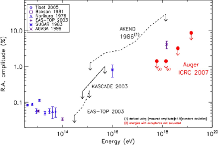
Figure 4: Summary of Auger 95% CL upper bounds on the amplitude of a dipolar modulation in right ascension and results from previous experiments.armengaud

As the energy increases and the number of events diminishes it becomes more difficult to measure the dipole amplitude. At energies higher than $10^{18}$ eV AGASA has found a Rayleigh amplitude of $4\%$. More recent results from the Pierre Auger Observatory have put upper bounds of $1.4\%$ above $10^{18}$ eV and $10\%$ above $10^{19}$ eV as it is shown in Figure 4.

2.0.2 Small and intermediate scale clustering

Clustering at small scales can be the clue to detect repeating sources. The amount of clustering (or the fraction of repeaters) gives a measure of the number of sources that contribute to the CRs above a given energy threshold, from which we can deduce the local density of sources. Clustering at intermediate angular scales contains information on the pattern of the distribution of the local sources.

The autocorrelation function

The autocorrelation function is a standard technique to analyse the distribution of points in the sky. It measures the excess (deficit) in the number of pairs with respect to that expected from an isotropic distribution as a function of the angle. For an isotropic distribution of $N$ points on the full celestial sphere the expected number of pairs with angle smaller than $\alpha$ is given by $n_{p}=(N(N-1)/2)(1-\cos(\alpha))$. For partial/non-uniform sky coverage the expected number of pairs from an isotropic flux has to be computed simulating isotropic event realizations following the exposure and counting the pairs as a function of the angle. The number of pairs separated by less than an angle $\alpha$ among the $N$ events with energy larger than a given threshold $E$ is

$$n_{p}(\alpha)=\sum_{i=2}^{N}\sum_{j=1}^{i-1}\Theta(\alpha-\alpha_{ij}),$$ (1)

where $\alpha_{ij}$ is the angular separation between events $i$ and $j$ and $\Theta$ is the step function. The chance probability for any excess of pairs at a fixed angle $\alpha$ and energy threshold is found from the fraction of simulations with a larger or equal number of pairs than what is found in the data at the angular scale of interest.

The results of the autocorrelation function analysis depend on the chosen values of $\alpha$ and $E$ (with the corresponding number of events $N$ above that energy threshold). The fact that the deflections expected from galactic and extragalactic magnetic fields and the distribution of the sources are largely unknown prevents to determine these values a priori. The significance of an autocorrelation signal at a given angle and energy, when these values have not been fixed a priori, is a delicate issue. A possible solution to this problem was proposed by Finley and Westerhoff FW , in which a scan over the energy threshold and the angular separation is performed. For each value of $N$ and $\alpha$, the fraction $f$ of simulations having an equal or larger number of pairs than the data is computed. The most relevant clustering signal corresponds to the values of $\alpha$ and $N$ that have the smallest value of $f$, referred to as $f_{min}$. To establish the statistical significance of a given excess, it is necessary to account for the fact that the angular bins, as well as the energy ones, are not independent. This can be done performing a large number of isotropic simulations with the same number of events as the data and calculate for each realisation the most significant deviation $f_{min}^{i}$. The statistical significance of the deviation from isotropy is the integral of the normalised $f_{min}$ distribution above $f_{min}^{data}$. Then the probability that such clustering arises by chance from an isotropic distribution can be estimated just from the fraction of simulations having $f_{min}^{i}\leq f_{min}^{data}$.

Although the data from a number of experiments have shown a remarkably isotropic distribution of arrival directions, there has been a claim of small scale clustering at energies larger than $40$ EeV by the AGASA experiment AGASA . The most recently published analysis teshima reports 8 pairs (five doublets and a triplet) with separation smaller than $2.5^{\circ}$ among the 59 events with energy above 40 EeV, while 1.7 were expected from an isotropic flux. The probability for this excess to happen by chance was estimated to be less than $10^{-4}$. The significance of the AGASA clustering result was, however, subject of debate based on the concern that the energy threshold and angular separation were not fixed a priori. Tinyakov and Tkachev TT01 computed the penalisation arising from making a scan in the energy threshold and obtained a probability of $3\times 10^{-4}$. Finley and Westerhoff FW took also into account the penalisation for a scan in the angular scale and obtained a probability of $3.5\times 10^{-3}$. The HiRes observatory has found no significant clustering signal at any angular scale up to $5^{\circ}$ for any energy threshold above $10$ EeV hires . A hint of correlation at scales around $25^{\circ}$ and energies above $40$ EeV, combining data from HiRes stereo, AGASA, Yakutsk and SUGAR experiments has been pointed out in ref.  KS .

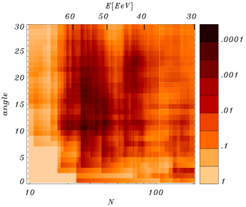
Figure 5: Autocorrelation scan

The Auger collaboration, using the events recorded by the surface detector between January 2004 and August 2007, has recently reported the results of the scan performed in energy (above 30 EeV, with 203 events detected) and angular separation (between 1^∘ and 30^∘) cris08 . The results are shown in the left panel of Figure 5. The most significant excess of pairs found is for $E>57$ EeV (corresponding to 27 events) and $\alpha=11^{\circ}$, with a chance probability of $P=1.6\times 10^{-2}$ to arise from an isotropic distribution. Above this energy, a broad region of low probabilities is observed, for angular scales between $9^{\circ}$ and $22^{\circ}$. The right panel of Figure 5 shows the number of observed pairs as a function of the angle (dots) as well as the expectations from an isotropic distribution with the 90$\%$ CL bars.

Search for point-like or extended excesses of events around a given direction in the sky

A neutral component of cosmic rays or a powerful source of charged particles at high energies could lead to a point-like excess of CRs arriving from the source direction. At lower energies charged particles can give rise to an extended excess of events from a region close to the source. Then it is important to have the tools to identify and estimate the significance of an excess of events from some region. The events coming from a source will be superimposed with that from the background, so we need to make an estimate of the signal and its significance.

For any given direction the first step is to measure the observed number of events in a window (that can be a top-hat, Gaussian, etc) around the given direction. For a point-like excess (as could arise for neutral primaries) the angular resolution size is considered. We call this number $N_{ON}$. Then we need to estimate the background. For this scope we can use the detector measurements in other regions of the sky, $N_{B}=\alpha N_{OFF}$ with $N_{OFF}$ the events measured in the $OFF$ region and $\alpha=t_{ON}/t_{OFF}$ = $\omega_{ON}/\omega_{OFF}$. From this we can estimate the signal as $N_{S}=N_{ON}-\alpha N_{OFF}$. To estimate the significance, one possibility is to use the variance of the signal. As $N_{ON}$ and $N_{OFF}$ are independent measurements, $\sigma^{2}(N_{S})=\sigma^{2}(N_{ON})+\alpha^{2}\sigma^{2}(N_{OFF}).$ Then there are different possibilities to estimate the variances. One possibility is to just consider two Poisson processes, then $\hat{\sigma}_{1}(N_{S})=\sqrt{N_{ON}+\alpha^{2}N_{OFF}}$ and the significance of the excess is given by $S_{1}=(N_{ON}-\alpha N_{OFF})/\sigma_{1}(N_{S})$. Another possibility is to consider that to estimate the significance of an excess what we want is to asses the probability that it arises only from the background. Then we would take for the pdf of $N_{ON}$ a Poisson distribution with mean equal to $\langle N_{B}\rangle$ and for $N_{OFF}$ a Poisson distribution with mean $\langle N_{B}\rangle/\alpha$. Then the variance is given by $\sigma^{2}(N_{S})=\langle N_{B}\rangle(1+\alpha)$ and estimating $\langle N_{B}\rangle=t_{ON}(N_{ON}+N_{OFF})/(t_{ON}+t_{OFF})=(N_{ON}+N_{OFF})\alpha/(1+\alpha)$, we have $\hat{\sigma}_{2}(N_{S})=\sqrt{\alpha(N_{ON}+N_{OFF})}$ and $S_{2}=(N_{ON}-\alpha N_{OFF})/\sigma_{2}(N_{S})$. An observed excess $N_{S}$ can be said to be an ’S standard deviation detection’. If $N_{ON}$ and $N_{OFF}$ are not too low ($\geq 10$), under the assumption that all the events come from the background ($\langle N_{S}\rangle=0$), the distribution of $S$ approximates a Gaussian variable with zero mean and unit variance, and the Gaussian probability of $S$ can be taken as the confidence level of the observational result. Tests with numerical simulations indicates that $S_{2}$ is a better estimator than $S_{1}$ lima .

Another proposal to estimate the significance is to use a likelihood ratio method (Li-Ma lima ). The likelihood ratio of the ’null hypothesis’, corresponding here to no source ($\langle N_{S}\rangle=0$), and that all events are coming from the background, and the alternative tested hypothesis, corresponding to a non-vanishing source ($\langle N_{S}\rangle\neq 0$), is defined as

$\lambda=\frac{L(data|null\ hyp)}{L(data|alternative\ hyp)}=\frac{P(data|\langle N_{S}\rangle=0)}{P(data|\langle N_{S}\rangle\neq 0)}.$

If the null hypothesis is true and $N_{ON},N_{OFF}\geq 10$, then $\sqrt{-2\ln\lambda}$ is Gaussian distributed with $\sigma^{2}=1$. Writting

$P(data|\langle N_{S}\rangle=0)=P(N_{ON},N_{OFF}|\langle N_{S}\rangle=0,\langle N_{B}\rangle=\frac{\alpha}{1+\alpha}(N_{ON}+N_{OFF}))=$

$\ \ \ \ \ \ \ \ \ \ \ \ \ \ \ Poisson(N_{ON};\langle N_{ON}\rangle=\langle N_{B}\rangle)\ Poisson(N_{OFF};\langle N_{OFF}\rangle=\langle N_{B}\rangle/\alpha),$

$P(data|\langle N_{S}\rangle=N_{ON}-\alpha N_{OFF},\langle N_{B}\rangle=\alpha N_{OFF})=$

$\ \ \ \ \ \ \ \ \ \ \ \ \ \ \ Poisson(N_{ON};\langle N_{ON}\rangle=N_{ON})\ Poisson(N_{OFF};\langle N_{OFF}\rangle=N_{OFF}),$

we can compute $\lambda$ as

$\lambda=\bigg{[}\frac{\alpha}{1+\alpha}\bigg{(}\frac{N_{ON}+N_{OFF}}{N_{ON}}\bigg{)}\bigg{]}^{N_{ON}}\bigg{[}\frac{1}{1+\alpha}\bigg{(}\frac{N_{ON}+N_{OFF}}{N_{OFF}}\bigg{)}\bigg{]}^{N_{OFF}}.$

The Li-Ma significance $S=\sqrt{-2\ln\lambda}$ was shown to follow a Gaussian distribution better that $S_{1}$ and $S_{2}$ lima .

The search of excesses of flux from point-like and extended regions is common to both the Cosmic Ray and Gamma Ray astronomy fields. The selection of the $ON$ and $OFF$ is decided according to the observational data. For example, if a possible excess of cosmic rays from a predetermined direction in sky is tested, the rest of the sky can be used as the $OFF$ region to determine the background isotropic expectation and the significance. If a blind search of excesses at a given angular scale is performed in the whole sky, proceeding in the same way for each particular direction, a distribution of significances is obtained. If no sources are present, they follow a Gaussian distribution with unit variance.

Galactic center searches

A potential site for the acceleration of CRs in our Galaxy is the Galactic center region with its super massive black hole and high density of stars. Thus, it is an interesting region to look for an excess of events. The AGASA collaboration found a 4.5$\sigma$ excess ($observed/expected=506/413.6$) in a $20^{\circ}$ radius region close to the Galactic center region for the energy range $10^{18}$–$10^{18.4}$ eV. Being in the southern hemisphere, the Auger Observatory has a privileged view towards the galactic centre (GC), which passes at just $6^{\circ}$ from the zenith at the site. For the same region where AGASA found the excess, and the same energy range, Auger data led to $obs/exp=2116/2159.6$ gcenter , a result inconsistent with a large excess. Similarly, an excess reported by the SUGAR collaboration in a $5^{\circ}$ region slightly displaced from the GC was not confirmed by Auger. A map of overdensity significances on $5^{\circ}$ radius windows in the region around the GC is shown in fig. 6, together with the regions were the AGASA and SUGAR excesses were reported. The excesses present in this map are consistent with the expectations from fluctuations of an isotropic distribution.

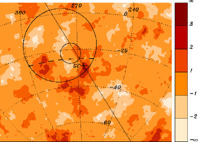
Figure 6: Map in equatorial coordinates around the GC (cross) showing the significance of the overdensities in $5^{\circ}$ radius windows, for $10^{17.9}{\rm eV}<E<10^{18.5}$ eV.

2.0.3 Searches for correlations with objects

Given a population of candidate sources there are different proposed tests to search for a correlation with CR arrival directions.

Cross-correlation function

This technique looks for an excess of CR separated by less than a given angle from any candidate source in the set with respect to the expectations from an isotropic CR distribution. The procedure is very similar to the autocorrelation analysis: we first count the number of pairs CR-objects as a function of the angle in the data. Then, we repeat the procedure for a large number of isotropic simulated data sets. To estimate the significance of any excess we compute the fraction of the simulations with larger number of pairs than those present in the data. This method was for example used to look for a possible correlation of CR with $E>10$ EeV and BL Lacs with magnitude $m<18$ at the experimental angular resolution scale (first found in HiRes data by Gorbunov et al. gor2004 ). In that magnitude range there are 156 BL Lacs in the field of view of HiRes in the Veron Cetty and Veron catalogue VC and 271 events have been reported by HiRes in that energy range. The number of observed pairs within $0.8^{\circ}$ was 11, while only 3 were expected from an isotropic distribution. The fraction of isotropic simulations with a larger number of pairs is $f(0.8^{\circ})=4\times 10^{-4}$. The penalization for searching at different angles and with different sets of objects is not included in that figure. A test of the signal using Auger data, with 1736 events with $E>10$ EeV showed no evidence of excess of correlation with BL Lacs with the same magnitude limit in the same catalogue harari2007 .

Maximum likelihood ratio method

The idea in this method is, for a given model of the source distribution, to find out the values of the parameters that lead to a better agreement with the observational data. For example, if the model considered is that a fraction of CRs events come from a known population of sources and another fraction from an isotropically distributed background, we would say that from the set of $N$ measured events, $n_{s}$ are source events and $N-n_{s}$ are background events. The probability that a background event arrives from any direction is proportional to the exposure $\omega(\hat{u})$. The probability that an event comes from one of the sources is peaked around the source direction $\hat{s}$ with some window $Q(\hat{u},\hat{s})$ given by the angular resolution of the experiment (for charged particles a larger spread can be introduced to account for magnetic deflections). For $M$ sources, the contribution of all the sources weighted by the exposure and eventually by a relative source intensity is added. For the simplest option of equally apparent bright sources we have

$$Q(\hat{u})=\sum_{j}\omega(\hat{s}_{j})Q(\hat{u},\hat{s}_{j})/\sum_{j}\omega(\hat{s}_{j}).$$

The probability distribution for any event is $P(\hat{u})=(n_{s}/N)Q(\hat{u})+(N-n_{s})/N\omega(\hat{u}).$ The likelihood for the set of $N$ events is $L(n_{s})=\prod_{i=1}^{N}P(\hat{u}_{i}).$ Then we search for the value of $n_{s}$ that maximizes the ratio $R(n_{s})=L(n_{s})/L(0)$, with $L(0)$ the likelihood of the null hypothesis ($n_{s}=0$). The significance can be estimated by computing $R$ for a large set of isotropic simulations and counting the fraction with $R_{sim}\geq R_{dat}$.

This method was used by HiRes to test the correlation of CRs with $E>10$ EeV with BL Lacs with $m<18$ at the resolution angular scale in their data Abbasi2005 . For each event $i$ they used for $Q(\hat{u}_{i},\hat{s}_{j})$ a Gaussian centred at $s_{j}$ with a dispersion equal to the angular resolution of that event. They found that $\ln R$ is maximized for $n_{s}=8.0$ corresponding to $\ln R=6.08$. The fraction of simulations with higher $\ln R$ is $f=2\times 10^{-4}$. Thus, the results are similar in this case to those using the cross-correlation analysis. Some advantages of this method are that it can be adapted to give different weight to each candidate source, for example depending on the distance or known brightness in some band. It is also possible to consider different angular scales depending on the angular resolution of the event, or e.g. from the expected magnetic deflections in different directions.

Binomial probability scan

For a given candidate source population, e. g. AGNs, galaxy clusters, radio galaxies, there are different parameters that will influence the correlation with events but that are difficult to fix a priori: the angular scale (magnetic deflections are not known), maximum distance to the objects (UHECR from distant sources will have their energy diminished by interactions with CMB through the GZK effect), energy threshold (only high energy events are expected to be correlated with local sources). The idea behind this method is to scan in the unknown parameters. For a given candidate source population, we can estimate the probability that an individual event from an isotropic flux has an arrival direction closer than some particular angular distance $\Psi$ from a member of the catalog, $p$, by computing the exposure-weighted fraction of the sky which is covered by windows of radius $\Psi$ centered on the selected objects. This will be a function of angular scale $\Psi$ and the maximum distance to the objects considered $D_{max}$, $p(\Psi,D_{max})$. For each energy threshold $E_{min}$, with $N$ events over the threshold, the number of events $k$ correlated to the sources is calculated. Then, the probability $P$ that $k$ or more events of the total of $N$ events are correlated by chance with the selected objects is given by the cumulative binomial probability

$$P=\sum_{j=k}^{N}\left(\matrix{N\cr j}\right)p^{\/j}(1-p)^{N-j}\leavevmode\nobreak\ .$$

The more significant correlation in the data set corresponds to the values $\Psi$, $E_{min}$ and $D_{max}$ that give rise to the smaller $P$ value, $P_{min}$. The significance of a given correlation can be estimated performing a large number of isotropic simulations and under the same scan in $\Psi$, $E_{min}$ and $D_{max}$ obtain the fraction $f$ having a $P_{min}$ smaller than the data.

Correlation of UHECR with AGNs

To test for possible correlations with extragalactic sources the Auger collaboration analyzed the arrival directions of the events above $4\times 10^{19}$ eV to look for coincidences with the positions of the known nearby (less than 100 Mpc) active galactic nuclei from the Veron-Cetty and Veron catalog ’citeVC. The results of a scan over the angle $\psi$ between the events and the AGNs, the maximum AGN redshift considered $z_{max}$ and the threshold energy $E_{th}$ show a deep minimum in the probability $P$ of observing a similar or larger number of correlations arising from isotropic simulated data. This minimum is obtained for $\psi=3.2^{\circ}$, $z_{max}=0.017$ (or maximum AGN distance of $71$ Mpc) and $E_{th}=57$ EeV (corresponding to the 27 highest energy events) science ; longagn . Only $\sim 10^{-5}$ of the isotropic simulations have a deeper minimum under a similar scan. In particular, for these 27 events 20 are at less than $3.2^{\circ}$ from an AGN closer than 71 Mpc, while only 6 were expected to be found by chance from an isotropic distribution of arrival directions. A correlation was first observed in the data obtained before the end of May 2006, with a very similar set of parameters, and fixing that set of parameters a priori the subsequent data up to August 2007 were studied, confirming the original correlation with more than 99% CL significance in the additional data set alone. This kind of prescribed test, using an independent data set and a priori fixed parameters, is the more safe strategy to prevent wrong claims with small statistics. It provides a clear way of assigning a significance to the observations, without relaying on penalizations for scanning.

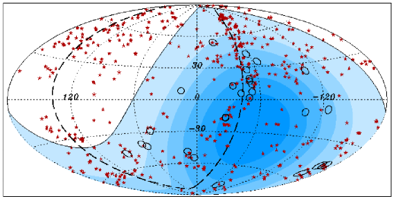
Figure 7: Map in galactic coordinates with the positions of the AGNs within 71 Mpc (stars) and the 27 events with $E>57$ EeV (circles of 3.2^∘ radius). Shading indicates regions of equal exposure science .

The map of the arrival directions and of the AGN positions is shown in Figure 7. A remarkable alignment of several events with the supergalactic plane (dashed line) is observed, and it is also worth noting that two events fall within 3.2^∘ from Centaurus A, the closest active galaxy. A further interesting fact is that the energy maximizing the correlation with AGNs coincides with that maximizing the autocorrelation of the events themselves cris08 and is also that for which the spectrum falls to half of the power law extrapolation from smaller energies spectrum .

Log likelihood per event

The previous method cannot be applied when the candidate source population is large, as the fraction of the sky covered, $p$, becomes of order unity. A more useful method in this case is to build a probability map for the expected arrival directions of events above a given threshold. The map can be constructed as follows, a Gaussian of given $\sigma$ is taken around the direction of each object in the catalog, weighting them by a factor

$$w(z,E_{th})=\frac{1}{4\pi d_{L}^{2}(z)\phi(z)}\int_{E_{i}(z,E_{th})}^{\infty}E^{-s}{\rm d}E.$$

where $d_{L}$ is the distance to the object, $\Phi(z)$ is the selection function of the catalog and the integral term measures the fraction of the flux from a source at redshift $z$ that reaches the Earth with an energy larger than the threshold $E_{th}$. $E_{i}$ is the initial energy that the particle needs to have at the source to arrive at Earth with $E_{th}$, $s$ is the source spectral index. As an example, the left panel of Figure 8 shows the map corresponding to the AGNs in the Veron-Cetty and Veron catalog and an energy threshold of 80 EeV.

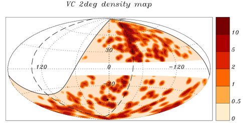
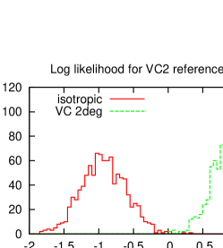
Figure 8: Likelihood map (left panel) and Log likelihood per event histograms (right panel)

The likelihood associated to a given set of $N$ observed events is $L=\prod_{i=1}^{N}P(\hat{u}_{i}),$ with $P(\hat{u}_{i})$ proportional to the map density in each event direction. In order that the mean value be independent of the total number of events, it is more convenient to use the log likelihood per event

$$LL=\frac{1}{N}\sum_{i=1}^{N}\ln P(\hat{u}_{i})$$

The idea is to measure $LL$ of the data using a model reference map. Then simulate events distributed according to some alternative hypothesis: isotropic, following AGNs,… and compute $LL$ for the reference model map. Then plot the histogram the $LLs$ for each hypothesis: the mean of the distribution is independent of the number $N$ of observed events, but the width becomes smaller as $N$ grows. When the histograms corresponding to the different hypothesis do not overlap the test is good to discriminate among them.

In the right panel of Figure 8 we show the histograms for 20 simulated isotropic events and for 20 events following the distribution of AGNs in the Veron-Cetty and Veron catalog using a Gaussian window of 2 degrees size.

3 Final remarks

A variety of different methods are needed to study anisotropies at different energies and angular scales. It is impossible to review in a limited space all the interesting ideas that have been put forward to this scope, I have only presented a (personally biased) subset of them, as well as a selection of the experimental results related to the techniques described.

This is a very special time for the field as the CR astronomy is finally starting and we are getting the first clues on the UHECR origin: they are correlated with nearby extragalactic matter. There are still many open questions as which are the sources, which is the CR composition, how are the relevant magnetic fields? More data is eagerly waited to clarify these issues.

References

- (1) J. L. Han, Magnetic fields of our Galaxy on large and small scales, IAU Symp.242 ‘Astrophysical Masers and their Environments’ Proceedings (2007) [astro-ph/0705.4175]; H. Men, K. Ferriere and J. L. Han, Observational constraints on models for the interstellar magnetic field in the Galactic disk, (2008) [astro-ph/0805.3454].
- (2) R. Beck, Galactic and extragalactic magnetic fields, astro-ph/0810.2923.
- (3) D. Harari, S. Mollerach and E. Roulet, JHEP 9908 (1999) 022 [arXiv:astro-ph/9906309].
- (4) D. Harari, S. Mollerach, E. Roulet and F. Sanchez, JHEP 0203 (2002) 045 [arXiv:astro-ph/0202362].
- (5) K. Greisen, Phys. Rev. Lett. 16 (1966) 748; G. T. Zatsepin and V. A. Kuzmin, JETP Lett. 4 (1966) 78.
- (6) D. Harari, S. Mollerach and E. Roulet, JCAP 0611 (2006) 012 [arXiv:astro-ph/0609294].
- (7) P. Sommers, Astropart. Phys. 14 (2001) 271. [arXiv:astro-ph/0004016].
- (8) J. Linsley, Phys. Rev. Lett. 34 (1975) 1530.
- (9) J. Aublin and E. Parizot, arXiv:astro-ph/0504575.
- (10) S. Mollerach and E. Roulet, JCAP 0508 (2005) 004 [arXiv:astro-ph/0504630].
- (11) M. Aglietta et al. [EAS-TOP Collaboration], Astrophys. J. 470 (1996) 501.
- (12) M. Amenomori et al. [The Tibet AS Gamma Collaboration], Phys. Rev. Lett. 93 (2004) 061101 [arXiv:astro-ph/0408187].
- (13) M. Amenomori et al. [Tibet AS Gamma Collaboration], arXiv:0711.2002 [astro-ph].
- (14) G. Guillian et al. [Super-Kamiokande Collaboration], Phys. Rev. D 75 (2007) 062003 [arXiv:astro-ph/0508468].
- (15) M. Amenomori [Tibet AS-gamma Collaboration], Science 314 (2006) 439 [arXiv:astro-ph/0610671].
- (16) E. Armengaud [Pierre Auger Collaboration], arXiv:0706.2640 [astro-ph].
- (17) C. B. Finley and S. Westerhoff, Astropart. Phys. 21 (2004) 359.
- (18) N. Hayashida et al. [AGASA Collaboration], Phys. Rev. Lett. 77 (1996) 1000.
- (19) M. Teshima et al. [AGASA Collaboration], Proc 28th ICRC, Tsukuba, Japan (2003), 437.
- (20) P. G. Tinyakov and I. I. Tkachev, JETP Lett. 74 (2001) 1 [Pisma Zh. Eksp. Teor. Fiz. 74 (2001) 3], arXiv:astro-ph/0102101.
- (21) R. U. Abbasi et al. [The High Resolution Fly’s Eye Collaboration (HIRES)], Astrophys. J. 610, L73 (2004).
- (22) M. Kachelriess and D. V. Semikoz, Astropart. Phys. 26 (2006) 10.
- (23) S. Mollerach [The Pierre Auger Collaboration], arXiv:0901.4699 [astro-ph].
- (24) T. P. Li and Y. Q. Ma, Astrophys. J. 272 (1983) 317.
- (25) M. Aglietta et al. [Pierre Auger Collaboration], Astropart. Phys. 27 (2007) 244 [arXiv:astro-ph/0607382].
- (26) D. S. Gorbunov, P. G. Tinyakov, I. I. Tkachev and S. V. Troitsky, JETP Lett. 80 (2004) 145 [Pisma Zh. Eksp. Teor. Fiz. 80 (2004) 167] [arXiv:astro-ph/0406654].
- (27) M.-P. Véron-Cetty and P. Véron, Astron. and Astrophys. 455 (2006) 773.
- (28) D. Harari [The Pierre Auger Collaboration], arXiv:0706.1715 [astro-ph].
- (29) R. U. Abbasi et al. [HiRes Collaboration], Astrophys. J. 636 (2006) 680 [arXiv:astro-ph/0507120].
- (30) J. Abraham et al. [Pierre Auger Collaboration], Science 318 (2007) 938 [arXiv:0711.2256 [astro-ph]].
- (31) J. Abraham et al. [Pierre Auger Collaboration], Astropart. Phys. 29 (2008) 188 [Erratum-ibid. 30 (2008) 45] [arXiv:0712.2843 [astro-ph]].
- (32) J. Abraham et al. [Pierre Auger Collaboration], Phys. Rev. Lett. 101 (2008) 061101 [arXiv:0806.4302 [astro-ph]].