An Interpolatory Estimate for the $\mathrm{UMD}$–Valued Directional Haar Projection

1. Main Results

1.1. A Brief History of Developement

The Calculus of Variations, in particular the theory of compensated compactness has long been a source of hard problems in harmonic analysis. One developement started with the work of F. Murat and L. Tartar and especially in the papers of Murat ([Tar78, Tar79, Tar83, Tar84, Tar90, Tar93], and [Mur78, Mur79, Mur81]). The decicive theorems were on Fourier multipliers of Hörmander type. For extensions of the use of Fourier multipliers in relation to sequential weak lower semicontinuity of integrals of the form

$$(u,v)\mapsto\int f(x,u(x),v(x))\,\mathrm{d}x,$$

and Young Measures and a full developement of the method see [FM99]. The extensions are due to S. Mueller (see [Mue99]), who used time–frequency localization and modern Calderon–Zygmund theory to strengthen the results obtained by Fourier multiplier methods.

Let $u\in L^{p}(\mathbb{R}^{n})$, with $n\geq 2$ and $1<p<\infty$ fixed, then the directional Haar projection $P^{(\varepsilon)}\,:\,L^{p}(\mathbb{R}^{n})\longrightarrow L^{p}(\mathbb{R}^{n})$, is given by

$$P^{(\varepsilon)}u=\sum_{Q\in\mathscr{Q}}\langle u,h_{Q}^{(\varepsilon)}\rangle\,h_{Q}^{(\varepsilon)}\,|Q|^{-1}.$$

For a precise definition see (4.1). In [Mue99] S. Mueller obtained the result

$$\|P^{(\varepsilon)}u\|_{L^{2}(\mathbb{R}^{2})}\leq C\,\|u\|_{L^{2}(\mathbb{R}^{2})}^{1/2}\,\|R_{i_{0}}u\|_{L^{2}(\mathbb{R}^{2})}^{1-1/2},$$ (1.1)

where $R_{i_{0}}$ denotes the $i_{0}$–th Riesz transform in $\mathbb{R}^{2}$, $0\neq(\varepsilon_{1},\varepsilon_{2})=\varepsilon\in\{0,1\}^{2}$, and $\varepsilon_{i_{0}}=1$. The formal definition of the Riesz transform is supplied in section 2.

This inequality was then extended by J. Lee, P. F. X. Mueller and S. Mueller in [LMM07] to arbitrary $1<p<\infty$ and dimensions $n\geq 2$ to

$$\|P^{(\varepsilon)}u\|_{L^{p}(\mathbb{R}^{n})}\leq C\,\|u\|_{L^{p}(\mathbb{R}^{n})}^{1/\min(2,p)}\,\|R_{i_{0}}u\|_{L^{p}(\mathbb{R}^{n})}^{1-1/\min(2,p)},$$ (1.2)

where $\varepsilon\in\{0,1\}^{n}\setminus\{0\}$, $\varepsilon_{i_{0}}=1$. Note that the behaviour of this inequality for $1<p<2$ and $2<p<\infty$ strongly varies. The most important application of (1.2) appears for $p=n$. One can rewrite (1.2) using the notion of type $\cal T(L^{p}(\mathbb{R}^{n}))=\min(2,p)$

$$\|P^{(\varepsilon)}u\|_{L^{p}(\mathbb{R}^{n})}\leq C\,\|u\|_{L^{p}(\mathbb{R}^{n})}^{1/\cal T(L^{p}(\mathbb{R}^{n}))}\,\|R_{i_{0}}u\||_{L^{p}(\mathbb{R}^{n})}^{1-1/\cal T(L^{p}(\mathbb{R}^{n}))}.$$

The proofs of (1.1) as well as (1.2) are based on two consecutive and ad hoc defined time–frequency localizations of the operator $P^{(\varepsilon)}$, based on Littlewood–Paley and wavelet expansions.

1.2. The Main Result

S. Mueller asks in [Mue99] whether it is possible to obtain (1.1) in such a way that the original time–frequency decompositions are replaced by the canonical martingale decomposition of T. Figiel (see [Fig88] and [Fig91]). This paper provides an affirmative answer to this question, and thus extending the interpolatory estimate (1.2) to the Bochner–Lebesgue space $L_{X}^{p}(\mathbb{R}^{n})$, provided $X$ satisfies the $\mathrm{UMD}$–property.

Our methods are based on martingale methods, explaining the behaviour of the exponents in the following main inequality 1.3 in terms of type and cotype. The main result of this paper reads as follows.

Theorem (Main Result).

Let $1<p<\infty$, $1\leq i_{0}\leq n$ and $\varepsilon=(\varepsilon_{1},\ldots,\varepsilon_{n})\in\{0,1\}^{n}$ such that $\varepsilon_{i_{0}}=1$. If $X$ has the $\mathrm{UMD}$–property and $L_{X}^{p}$ has non–trivial type $\cal T(L_{X}^{p})$, then there exists a constant $C$, such that for all $u\in L_{X}^{p}$

$$\|P^{(\varepsilon)}u\|_{L_{X}^{p}}\leq C\ \|u\|_{L_{X}^{p}}^{1/\cal T(L_{X}^{p})}\,\|R_{i_{0}}u\|_{L_{X}^{p}}^{1-1/\cal T(L_{X}^{p})},$$ (1.3)

whereas the constant $C$ depends only on $n$, $p$, $X$ and $\cal T(L_{X}^{p})$.

Proof.

First define $M\in\mathbb{N}$ by

$$2^{M-1}\leq\frac{\|R_{i_{0}}\|_{L_{X}^{p},L_{X}^{p}}\,\|u\|_{L_{X}^{p}}}{\|R_{i_{0}}u\|_{L_{X}^{p}}}\leq 2^{M}.$$ (1.4)

After using decomposition (4.2), the triangle inequality, estimates (4.36), (4.14), (4.37) and plugging in $M$, we obtain

$$\|P^{(\varepsilon)}u\|_{L_{X}^{p}} \leq\|P_{-}^{(\varepsilon)}R_{i_{0}}^{-1}R_{i_{0}}u\|_{L_{X}^{p}}+\sum_{l=0}^{M}\|P_{l}R_{i_{0}}^{-1}R_{i_{0}}u\|_{L_{X}^{p}}+\sum_{l=M}^{\infty}\|P_{l}u\|_{L_{X}^{p}}$$

$$\lesssim\|R_{i_{0}}u\|_{L_{X}^{p}}+\sum_{l=0}^{M}2^{l/\cal T(L_{X}^{p})}\,\|R_{i_{0}}u\|_{L_{X}^{p}}+\sum_{l=M}^{\infty}2^{-l(1-\frac{1}{\cal T(L_{X}^{p})})}\,\|u\|_{L_{X}^{p}}$$

$$\lesssim 2^{M/\cal T(L_{X}^{p})}\,\|R_{i_{0}}u\|_{L_{X}^{p}}+2^{-M(1-\frac{1}{\cal T(L_{X}^{p})})}\,\|u\|_{L_{X}^{p}}$$

$$\leq C\,\|u\|_{L_{X}^{p}}^{1/\cal T(L_{X}^{p})}\|R_{i_{0}}u\|_{L_{X}^{p}}^{1-1/\cal T(L_{X}^{p})}.$$

∎

The basic tools for the proof of the above theorem are vector–valued estimates of so called ring domain operators, developed in section 3. A careful examination of T. Figiel’s shift operators acting on ring domains will be crucial in those estimates.

Clearly, the main result, theorem Theorem, represents a result on interpolation of operators, linking the identity map, the Riesz transforms and the directional Haar projection. We would now like to give a reformulation of our main theorem which places it in the context of structure theorems for the so called $K$–method of interpolation spaces. To this end, we first introduce the $K$–functional, cite the relevant structure theorem and apply it to the inequalities stated as our main result.

Define the $K$–functional

$$K(f,t)=\inf\big{\{}\|g\|_{E_{0}}+t\,\|h\|_{E_{1}}\,:\,f=g+h,\ g\in E_{0},h\in E_{1}\big{\}},$$

for all $f\in E_{0}+E_{1}$ and $t>0$, and the interpolation space

$$(E_{0},E_{1})_{\theta,1}=\big{\{}f\,:\,f\in E_{0}+E_{1},\ \|f\|_{\theta,1}<\infty\big{\}},$$

where

$$\|f\|_{\theta,1}=\int_{0}^{\infty}t^{-\theta}\,K(f,t)\,\frac{\mathrm{d}t}{t}.$$

The following proposition interprets interpolatory estimates such as the ones obtained in our main theorem in terms of continuity of the identity map between interpolation spaces. The following proposition is a result of general interpolation theory (see [BS88, Proposition 2.10, Chapter 5]).

Proposition 1.1.

Let $(E_{0},E_{1})$ be a compatible couple and suppose $0<\theta<1$. Then the estimate

$$\|f\|_{E}\leq C\,\|f\|_{\theta,1}$$ (1.5)

holds for some constant $C$ and all $f$ in $(E_{0},E_{1})_{\theta,1}$ if and only if

$$\|f\|_{E}\leq C\,\|f\|_{E_{0}}^{1-\theta}\,\|f\|_{E_{1}}^{\theta}$$

holds for some constant $C$ and for all $f$ in $E_{0}\cap E_{1}$.

Now we specify how to choose the spaces $E$, $E_{0}$ and $E_{1}$ so that the two equivalent conditions of the above proposition match precisely the assertions of our main theorem, see inequality (1.3).

Fix $0\neq\varepsilon\in\mathbb{\{}0,1\}^{n}$, let $R$ denote one of the Riesz transform operators

$$R_{i}\,:\,L_{X}^{p}\rightarrow L_{X}^{p}$$

defined in section 2, where $\varepsilon_{i}=1$, and abbreviate $P^{(\varepsilon)}$ by $P$. If we define the Banach spaces

$$E =L_{X}^{p}/\ker(P), \|u+\ker(P)\|_{E} =\|Pu\|_{L_{X}^{p}},$$

$$E_{0} =L_{X}^{p}, \|u\|_{E_{0}} =\|u\|_{L_{X}^{p}},$$

$$E_{1} =L_{X}^{p}/\ker(R), \|u+\ker(R)\|_{E_{1}} =\|Ru\|_{L_{X}^{p}},$$

then in view of proposition 1.1

$$(E_{0},E_{1})_{\theta,1}\hookrightarrow E,$$

is equivalent to the existence of a constant $C>0$ such that

$$\|u\|_{E}\leq C\,\|u\|_{\theta,1},$$

for all $u\in(E_{0},E_{1})_{\theta,1}$.

We are grateful to S. Geiss who pointed out the connection to general interpolation theory.

2. Preliminaries

This brief section will provide notions and tools most frequently used in what follows.

At first we will introduce the Haar system supported on dyadic cubes, the notions of Banach spaces with the $\mathrm{UMD}$–property and type and cotype of Banach spaces. The $\mathrm{UMD}$–property enables us to introduce Rademacher means in our norm estimates, so that we may use the subsequent inequalities, that is Kahane’s inequality, Kahane’s contraction principle and Bourgain’s version of Stein’s martingale inequality.

Then we turn to Figiel’s shift operators $T_{m}$ acting on all of the Haar system, where $T_{m}$ is bounded by a constant multiple of

$$\log(2+|m|),\qquad m\in\mathbb{Z}^{n}.$$

Very roughly speaking this result due to T. Figiel is obtained by partitioning all of the dyadic cubes into $\log(2+|m|)$ collections and bounding $T_{m}$ by a constant on each of the collections. We will have to consider $T_{m}$ acting only in one direction (assume $m_{2}=\ldots=m_{n}=0$) on the Haar spectrum of certain ring domain operators $S_{\lambda}$, $\lambda\geq 0$, and it turns out that $T_{m}$ restricted to this spectrum is uniformly bounded by a constant, as long as $0\leq m_{1}\leq 2^{\lambda}-1$.

The Haar System

First we consider the collection of dyadic intervals at scale $j\in\mathbb{Z}$

$$\mathscr{D}_{j}=\big{\{}\ [2^{-j}k,2^{-j}(k+1)[\,:\,k\in\mathbb{Z}\ \big{\}},$$

and the collection of all dyadic intervals

$$\mathscr{D}=\bigcup_{j\in\mathbb{Z}}\mathscr{D}_{j}.$$

Now define the $L^{\infty}$–normalized Haar system

$$h_{[0,1[}(t) =\mathtt{1}_{[0,\frac{1}{2}[}(t)-\mathtt{1}_{[\frac{1}{2},1[}(t), t \in\mathbb{R}$$

and for any $$I\in\mathscr{D}$$

$$h_{I}(t) =h_{[0,1[}\big{(}\frac{t-\inf I}{|I|}\big{)}, t \in\mathbb{R}.$$

In arbitrary dimensions $n\geq 2$ one can obtain a basis for $L^{p}(\mathbb{R}^{n})$ as follows. For any $\varepsilon=(\varepsilon_{1},\ldots,\varepsilon_{n})\in\{0,1\}^{n}$, $\varepsilon\neq 0$ define

$$h^{(\varepsilon)}_{Q}(t)=\prod_{i=1}^{n}h_{I_{i}}^{\varepsilon_{i}}(t_{i}),$$

where $t=(t_{1},\ldots,t_{n})\in\mathbb{R}^{n}$, $Q=I_{1}\times\cdots\times I_{n}$, $|I_{1}|=\ldots=|I_{n}|$, $I_{i}\in\mathscr{D}$, and by $h_{I_{i}}^{\varepsilon_{i}}$ we mean

$$h_{I_{i}}^{\varepsilon_{i}}=\begin{cases}h_{I_{i}}&\varepsilon_{i}=1\\ \mathtt{1}_{I_{i}}&\varepsilon_{i}=0\end{cases}$$

Note that the former basis is supported on rectangles $R$, but the latter basis is supported on dyadic cubes $Q$.

Banach Spaces with the $\mathrm{UMD}$–Property

By $L^{p}(\Omega,\mu;X)$ we denote the space of functions with values in $X$, Bochner–integrable with respect to $\mu$. If $\Omega=\mathbb{R}^{n}$ and $\mu$ is the Lebesgue measure $|\cdot|$ on $\mathbb{R}^{n}$, then set $L_{X}^{p}(\mathbb{R}^{n})=L^{p}(\mathbb{R}^{n},|\cdot|;X)$, if unambiguous abbreviated as $L_{X}^{p}$.

We say $X$ is a $\mathrm{UMD}$ space if for any $X$–valued martingale difference sequence $\{d_{j}\}_{j}\subset L^{p}(\Omega,\mu;X)$ and any choice of signs $\varepsilon_{j}\in\{-1,1\}$ one has

$$\big{\|}\sum_{j}\varepsilon_{j}\,d_{j}\big{\|}_{L^{p}(\Omega,\mu;X)}\leq\mathscr{U}_{p}(X)\,\big{\|}\sum_{j}d_{j}\big{\|}_{L^{p}(\Omega,\mu;X)}.$$ (2.1)

A Banach space $X$ is said to be of type $\cal T$, $1<\cal T\leq 2$, respectively of cotype $\cal C$, $2\leq\cal C<\infty$ if there are constansts $A(\cal T,X)>0$ and $B(\cal C,X)>0$, such that for every finite set of vectors $\{x_{j}\}_{j}\subset X$ we have

$$\int_{0}^{1}\big{\|}\sum_{j}r_{j}(t)\,x_{j}\big{\|}_{X}\,\mathrm{d}t \leq A(\cal T,X)\,\big{(}\sum_{j}\|x_{j}\|_{X}^{\cal T}\big{)}^{1/\cal T},$$ (2.2)

respectively

$$\int_{0}^{1}\big{\|}\sum_{j}r_{j}(t)\,x_{j}\big{\|}_{X}\,\mathrm{d}t \geq B(\cal C,X)\,\big{(}\sum_{j}\|x_{j}\|_{X}^{\cal C}\big{)}^{1/\cal C},$$ (2.3)

where $\{r_{j}\}_{j}$ is an independent sequence of Rademacher functions.

It is well known that if $X$ is a $\mathrm{UMD}$–space, then for every $1<p<\infty$ the Lebesgue–Bochner space $L_{X}^{p}$ has (non–trivial) type and cotype. Since inequality (2.2) holds for $\cal T=1$, respectively inequality (2.3) with $\cal C=\infty$, even if $X$ does not have the $\mathrm{UMD}$–property, one often refers to $\cal T=1$ as trivial type, respectively to $\cal C=\infty$ as trivial cotype.

Kahane’s Inequality

Given $1\leq p<\infty$, there exists a constant $K_{p}$ such that for any Banach space $X$ and any finite sequence $\{x_{j}\}\subset X$ holds that

$$\bigg{(}\int_{0}^{1}\Big{\|}\sum_{j}r_{j}(t)\,x_{j}\Big{\|}_{X}^{p}\,\mathrm{d}t\bigg{)}^{1/p}\leq K_{p}\,\int_{0}^{1}\Big{\|}\sum_{j}r_{j}(t)\,x_{j}\Big{\|}_{X}\,\mathrm{d}t,$$ (2.4)

where $\{r_{j}\}_{j}$ denotes an independent sequence of Rademacher functions.

Kahane’s Contraction Principle

For any Banach space $X$, $1<p<\infty$, finite set $\{x_{j}\}\subset X$ and bounded sequence of scalars $\{c_{j}\}$ holds true

$$\int_{0}^{1}\Big{\|}\sum_{j}r_{j}(t)\,c_{j}\,x_{j}\Big{\|}_{X}^{p}\,\mathrm{d}t\leq\sup_{j}|c_{j}|^{p}\,\int_{0}^{1}\Big{\|}\sum_{j}r_{j}(t)\,x_{j}\Big{\|}_{X}^{p}\,\mathrm{d}t,$$ (2.5)

where $\{r_{j}\}_{j}$ denotes an independent sequence of Rademacher functions.

The Martingale Inequality of Stein – Bourgain’s Version

The vector–valued version of Stein’s martingale inequality states that if $(\Omega,\cal F,\mu)$ is a probability space, $\cal F_{1}\subset\ldots\subset\cal F_{m}\subset\cal F$ is an increasing sequence of $\sigma$–algebras, $f_{1},\ldots,f_{m}\in L^{p}(\Omega,\mu;X)$ and $r_{1},\ldots,r_{m}$ are independent Rademacher functions, then

$$\int_{0}^{1}\big{\|}\sum_{i=1}^{m}r_{i}(t)\,\operatorname{\mathbb{E}}(f_{i}|\cal F_{i})\big{\|}_{L^{p}(\Omega,\mu;X)}\,\mathrm{d}t\leq C\,\int_{0}^{1}\big{\|}\sum_{i=1}^{m}r_{i}(t)\,f_{i}\big{\|}_{L^{p}(\Omega,\mu;X)}\,\mathrm{d}t,$$ (2.6)

where $C$ depends on $p$ and $X$. The Banach space $X$ having the $\mathrm{UMD}$–property assures $C<\infty$.

Figiel’s Shift Operators

The proof of the main result (1.3) makes use of Figiel’s shift operators [Fig88]. For any $m\in\mathbb{Z}^{n}$, and collection $\mathscr{B}$ of cubes $Q\subset\mathbb{R}^{n}$ let $\tau_{m}\,:\,\mathscr{B}\rightarrow\mathscr{Q}$

$$\tau_{m}(Q)=Q+m\,\operatorname{sl}(Q),$$ (2.7)

where $\operatorname{sl}(Q)$ is the sidelength of $Q$. Precisely, if $Q=I_{1}\times\ldots\times I_{n}$, with $|I_{1}|=\ldots=|I_{n}|$, then $\operatorname{sl}(Q)=|I_{1}|=\ldots=|I_{n}|$.

The map $\tau_{m}$ induces the rearrangement operator $T_{m}$, as the linear extension of

$$T_{m}h_{Q}=h_{\tau_{m}(Q)},\qquad Q\in\mathscr{B}.$$ (2.8)

Let $X$ be a $\mathrm{UMD}$ space, then the theorem of T. Figiel bounds the shift operator $T_{m}$ acting on $L_{X}^{p}$ by

$$\|T_{m}\,:\,L_{X}^{p}\rightarrow L_{X}^{p}\|\leq C\,\log(2+|m|),$$ (2.9)

where $C=C(n,p,\mathscr{U}_{p}(X))$.

The Riesz Transform

Formally, we define the Riesz transform $R_{i_{0}}$ by

$$R_{i_{0}}f =K_{i_{0}}*f,$$ (2.10)

$$K_{i_{0}}(x) =c_{n}\,\frac{x_{i_{0}}}{|x|^{n+1}}, x =(x_{1},\ldots,x_{n}).$$ (2.11)

Details may be found in [Ste70] and [Ste93].

Supplementary Definitions

$$\cal E=\cal E(n)=\big{\{}\varepsilon\in\{0,1\}^{n}\,:\,\varepsilon\neq(0,\ldots,0)\big{\}},$$

and

$$\cal E_{i_{0}}=\cal E_{i_{0}}(n)=\big{\{}\varepsilon\in\{0,1\}^{n}\,:\,\varepsilon_{i_{0}}\neq 0\big{\}}.$$

For any operator $T:L_{X}^{p}\rightarrow L_{X}^{p}$, the Haar–spectrum is defined by

$$\mathscr{Q}\setminus\big{\{}Q\in\mathscr{Q}\,:\,\langle Tu,h_{Q}^{(\varepsilon)}\rangle=0,\text{for all $u\in L_{X}^{p}$ and $\varepsilon\in\cal E$}\big{\}}.$$ (2.12)

Given a collection of sets $\mathscr{C}$, we denote

$$\sigma(\mathscr{C})=\bigcap\big{\{}\mathscr{A}\,:\,\text{$\mathscr{A}$ is a $\sigma$--algebra},\mathscr{C}\subset\mathscr{A}\big{\}},$$

the smallest $\sigma$–algebra containing $\mathscr{C}$.

3. The Ring Domain Operator $S_{\lambda}$

Here we define and study the ring domain operators $S_{\lambda}$, mapping $u\in L_{X}^{p}$ onto the blocks $\operatorname{lin}\big{\{}g_{Q,\lambda}\,:\,Q\in\mathscr{Q}\big{\}}$, each supported on a ring–shaped structure, see figure 1, from now on referred to as ring domain. The vector–valued estimates for these operators constitute the technical main component of this paper.

The main result for the ring domain operator is stated in theorem 3.3.

3.1. Preparation

Now we turn to defining ring domains and their corresponding ring domain operators. Within this section the superscripts $\varepsilon$ are omitted, we assume $\lambda\geq 0$ and generically denote $h_{Q}$ one of the functions $\{h_{Q}^{(\varepsilon)}\}_{\varepsilon\neq 0}$.

Let $D(Q)$ be the set of discontinuities of the Haar function $h_{Q}$, then

$$D_{\lambda}(Q)=\{x\in\mathbb{R}^{n}\,:\,\operatorname{dist}(x,D(Q))\leq C\,2^{-\lambda}\,\operatorname{diam}(Q)\}.$$

First note that

$$|D_{\lambda}(Q)|\lesssim 2^{-\lambda}\,|Q|.$$ (3.1)

Now we cover the set $D_{\lambda}(Q)$ using dyadic cubes $E(Q)$ having diameter

$$\operatorname{diam}(E(Q))=2^{-\lambda}\,\operatorname{diam}(Q),$$

and call the collection of those cubes $\cal U_{\lambda}(Q)$. More precisely,

$$\cal U_{\lambda}(Q)=\big{\{}E\in\mathscr{Q}\,:\,\operatorname{diam}(E)=2^{-\lambda}\operatorname{diam}(Q),\,E\cap D_{\lambda}(Q)\neq\emptyset\big{\}}.$$ (3.2)

The pointset $U_{\lambda}(Q)$ covered by $\cal U_{\lambda}(Q)$ is illustrated by the shaded region in figure 1, wherein the dashed lines represent the set of discontinuities $D(Q)$.

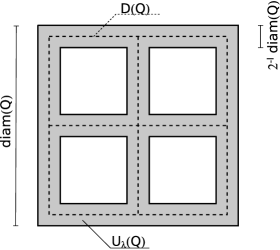
Figure 1. Ring domain (shaded region).

The cardinality $\operatorname{\#}\cal U_{\lambda}(Q)$ does not depend on the choice of $Q$, precisely

$$\operatorname{\#}\cal U_{\lambda}(Q)\approx 2^{\lambda(n-1)}.$$ (3.3)

Now we define the functions $g_{Q,\lambda}$ associated to the ring domain $\cal U_{\lambda}(Q)$ as

$$g_{Q,\lambda}=\sum_{E\in\cal U_{\lambda}(Q)}h_{E}.$$ (3.4)

The ring domain operator onto $\operatorname{lin}\big{\{}g_{Q,\lambda}\,:\,Q\in\mathscr{Q}\big{\}}$ is then given by:

$$S_{\lambda}u=\sum_{Q\in\mathscr{Q}}\langle u,h_{Q}\rangle\,g_{Q,\lambda}|Q|^{-1}.$$ (3.5)

The main tools for analyzing $S_{\lambda}$ are on one hand Figiel’s shift operators $T_{m}$, $m\in\mathbb{Z}^{n}$, defined as linear extension of the map

$$T_{m}h_{Q}=h_{Q+m\,\operatorname{sl}(Q)},$$

and on the other hand Bourgain’s version of Stein’s martingale inequality.

Before beginning to analyze our ring domain operator $S_{\lambda}$, we decompose $g_{Q,\lambda}$ into a sum of no more than $3n$ functions, well localised in the vicinity of the set of the discontinuities of the Haar function $h_{Q}$. So for any $Q\in\mathscr{Q}$ we partition

$$\cal U_{\lambda}(Q)=\bigcup_{i=1}^{3n}\cal U_{\lambda}^{(i)}(Q),$$

such that for all $E\in\cal U_{\lambda}^{(i)}(Q)$ holds

$$\cal U_{\lambda}^{(i)}(Q)\subset\big{\{}E+j\,u_{i}\,:\,j\in\mathbb{Z}\big{\}},$$

where $u_{i}$ is one of the standard unit vectors of $\mathbb{R}^{n}$. This partition induces a splitting of the blocks $g_{Q,\lambda}$ into

$$g_{Q,\lambda}=\sum_{i=1}^{3n}g_{Q,\lambda}^{(i)}.$$

We denote one of the functions $g_{Q,\lambda}^{(i)}$ decomposing $g_{Q,\lambda}$ generically by $g_{Q,\lambda}$ again, and we may assume that the support of $g_{Q,\lambda}$ is aligned orthogonal to $e_{1}\in\mathbb{R}^{n}$, where $e_{1}=(1,0,\ldots,0)$. We split the operator $S_{\lambda}$ accordingly, and denote the operator aligned orthogonal to $e_{1}$ by $S_{\lambda}$ again. So we have analogously to equation (3.5)

$$S_{\lambda}u=\sum_{Q\in\mathscr{Q}}\langle u,h_{Q}\rangle\,g_{Q,\lambda}|Q|^{-1},$$

with the support of $g_{Q,\lambda}$ now beeing localized in the vicinity of just one of the $3$ faces of $D(Q)$ perpendicular to $e_{1}$.

Recalling (2.8) it is easy to see that for any $u=\sum_{Q\in\mathscr{Q}}u_{Q}\,h_{Q}\,|Q|^{-1}\in L_{X}^{p}$ one can find functions $\{c_{Q}\}_{Q\in\mathscr{Q}}$, $|c_{Q}|=1$ such that

$$\sum_{Q\in\mathscr{Q}}c_{Q}\,u_{Q}\,h_{Q}\,|Q|^{-1}=\sum_{m=0}^{2^{\lambda}-1}T_{m\,e_{1}}S_{\lambda}u=\sum_{m=0}^{2^{\lambda}-1}S_{\lambda}^{m}u,$$

where we defined

$$S_{\lambda}^{m}u=T_{m\,e_{1}}S_{\lambda}u.$$ (3.6)

Precisely, $c_{Q}$ is given by

$$c_{Q}=h_{Q}\cdot\sum_{m=0}^{2^{\lambda}-1}T_{m\,e_{1}}g_{Q,\lambda}.$$

Note that the shifted support strips $U_{\lambda}(Q)$ of $T_{m\,e_{1}}g_{Q,\lambda}$, $0\leq m<2^{\lambda}$ cover the whole cube $Q$ (see figure 2).

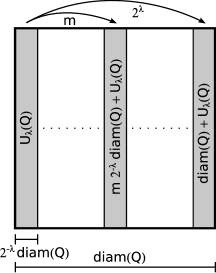
Figure 2. The thin blocks $g_{Q,\lambda}$ with shaded support $U_{\lambda}(Q)$ are shifted to cover the whole cube Q.

So the well known $\mathrm{UMD}$–property and Kahane’s contraction principle imply

$$\|u\|_{L_{X}^{p}}\approx\big{\|}\sum_{Q\in\mathscr{Q}}c_{Q}\,u_{Q}\,h_{Q}\,|Q|^{-1}\big{\|}_{L_{X}^{p}}=\big{\|}\sum_{m=0}^{2^{\lambda}-1}S_{\lambda}^{m}u\big{\|}_{L_{X}^{p}}.$$ (3.7)

3.2. Estimates for the Ring Domain Operator

The next Lemma analyzes the spectrum of $S_{\lambda}$ and prepares for the construction of atoms, used later in the martingale estimates for $S_{\lambda}$.

Before we state the lemma, we build up some notation. Let $\operatorname{\pi}_{\lambda}\,:\,\mathscr{D}\rightarrow\mathscr{D}$, and define for any $I\in\mathscr{D}$

$$\operatorname{\pi}_{\lambda}(I)=J,$$

where the uniquely determined $J\in\mathscr{D}$ is such that $|J|=2^{\lambda}\,|I|$ and $J\supset I$. Furthermore let

$$\mathscr{B}\subset\{I\in\mathscr{D}\,:\,\inf I=\inf\operatorname{\pi}_{\lambda}(I)\},$$

such that for all $J,K\in\mathscr{B}$ with $|J|\neq|K|$ holds that

$$|J|\leq\frac{1}{4}\,|K|\quad\text{or}\quad|K|\leq\frac{1}{4}\,|J|.$$

Lemma 3.1.

For any $\lambda\geq 1$ let $0\leq m\leq 2^{\lambda-1}$,

$$\tau(I)=I+m\,|I|,\qquad I\in\mathscr{D},$$

then

$$\big{|}I\cap\bigcup_{d=1}^{\lambda-1}\bigcup_{\begin{subarray}{c}J\in\mathscr{B}\\ |J|=2^{-d}\,|I|\end{subarray}}J\cup\tau_{m}(J)\big{|}\leq\frac{2}{3}\,|I|,$$

for all $I\in\mathscr{B}$.

Proof.

First we claim that for any $I\in\mathscr{B}\cup\tau_{m}(\mathscr{B})$, $1\leq d\leq\lambda-1$ and $J,K\in\mathscr{B}$ with $|J|=|K|=2^{-d}\,|I|$ holds

$$(J\cup\tau_{m}(J))\cap I\neq\emptyset\quad\text{and}\quad(K\cup\tau_{m}(K))\cap I\neq\emptyset\quad\text{implies}\quad J=K.$$ (3.8)

If we assume this claim does not hold true, then we can find intervals $J\neq K$ such that

$$(J\cup\tau_{m}(J))\cap I\neq\emptyset\quad\text{and}\quad(K\cup\tau_{m}(K))\cap I\neq\emptyset.$$

Since $J\neq K$ we know from the definition of $\mathscr{B}$ that

$$\operatorname{dist}(\tau_{m}(J),\tau_{m}(K))=\operatorname{dist}(J,K)\geq(2^{\lambda}-1)\,|J|,$$

consequently

$$\operatorname{dist}(J\cup\tau_{m}(J),K\cup\tau_{m}(K))\geq(2^{\lambda}-1-m)\,|J|.$$

Since $I$ intersects both $J\cup\tau_{m}(J)$ and $K\cup\tau_{m}(K)$, we infer

$$|I| \geq\operatorname{dist}(J\cup\tau_{m}(J),K\cup\tau_{m}(K))+2\,|J|$$

$$\geq(2^{\lambda}-m+1))\,2^{-d}\,|I|$$

$$\geq(2^{\lambda-1}+1)\,2^{-d}\,|I|$$

$$>|I|,$$

which is a contradiction. Hence (3.8) holds, wich means that if $1\leq d\leq\lambda-1$, any interval $I\in\mathscr{B}\cup\tau_{m}(\mathscr{B})$ intersects at most one of the sets

$$\{J\cup\tau_{m}(J)\in\mathscr{B}\,:\,|J|=2^{-d}\,|I|\}.$$

If such a $J$ exists we denote it by $J_{d}(I)\in\mathscr{B}$, and define $J_{d}(I)=\emptyset$ otherwise. Note that for small shift widths $m$ or small $J$ it may happen that $J_{d}(I)\cup\tau_{m}(J_{d}(I))\subset I$.

Using (3.8) we see that for every $I\in\mathscr{B}\cup\mathscr{\tau}_{m}(\mathscr{B})$

$$\big{|}I\cap\bigcup_{d=1}^{\lambda-1}\bigcup_{\begin{subarray}{c}J\in\mathscr{B}\\ |J|=2^{-d}\,|I|\end{subarray}}J\cup\tau_{m}(J)\big{|} =\sum_{d=1}^{\lambda-1}\big{|}I\cap\big{(}J_{d}(I)\cup\tau_{m}(J_{d}(I))\big{)}\big{|}$$

$$\leq\sum_{d=1}^{\lambda-1}2\cdot|J_{d}(I)|$$

$$\leq 2\cdot\sum_{d=1}^{\infty}2^{-2d}\,|I|$$

$$=\frac{2}{3}\,|I|.$$

The last inequality holds since for any $J,K\in\mathscr{B}$, $|J|\neq|K|$ implies $|J|\leq\frac{1}{4}|K|$ or $|K|\leq\frac{1}{4}|J|$, thus finishing the proof of the lemma. ∎

Having verified lemma 3.1, we now turn to prove the following pointwise estimates for $S_{\lambda}$. There exists a constant $C>0$ such that

$$\frac{1}{C}\,\|S_{\lambda}^{k}u\|_{L_{X}^{p}}\leq\|S_{\lambda}^{m}u\|_{L_{X}^{p}}\leq C\,\|S_{\lambda}^{k}u\|_{L_{X}^{p}},\qquad\lambda\geq 0,\ 0\leq k,m<2^{\lambda},\ u\in L_{X}^{p}.$$

Once more we emphazise that these estimates are crucial for the proof of the main result (1.3).

Proposition 3.2.

Let $X$ be a $\mathrm{UMD}$ space, $1<p<\infty$ and $n\in\mathbb{N}$. There exists $0<C<\infty$ such that for any $k,m,\lambda\in\mathbb{Z}$, with $\lambda\geq 0$, $0\leq k\leq 2^{\lambda}-1$ and $0\leq m\leq 2^{\lambda}-1$ the estimate

$$\frac{1}{C}\,\|S_{\lambda}^{k}u\|_{L_{X}^{p}}\leq\|S_{\lambda}^{m}u\|_{L_{X}^{p}}\leq C\,\|S_{\lambda}^{k}u\|_{L_{X}^{p}}$$ (3.9)

holds true for all $u\in L_{X}^{p}$. The constant $C$ depends on $n$, $p$ and $X$, particularly on the constant arising in Stein’s martingale inequality.

Proof.

In order to show (3.9), we will first prove

$$\frac{1}{C}\,\|S_{\lambda}^{0}u\|_{L_{X}^{p}}\leq\|S_{\lambda}^{m}u\|_{L_{X}^{p}}\leq C\,\|S_{\lambda}^{0}u\|_{L_{X}^{p}},$$ (3.10)

for all $\lambda\geq 0$ and $0\leq m\leq 2^{\lambda-1}$. Exploiting symmetry will also establish

$$\frac{1}{C}\,\|S_{\lambda}^{2^{\lambda}-1}u\|_{L_{X}^{p}}\leq\|S_{\lambda}^{m}u\|_{L_{X}^{p}}\leq C\,\|S_{\lambda}^{2^{\lambda}-1}u\|_{L_{X}^{p}},$$ (3.11)

for all $\lambda\geq 0$ and $2^{\lambda-1}-1\leq m\leq 2^{\lambda}-1$. Once we have (3.10) and (3.11), we gain (3.9), since all operators $\{S_{\lambda}^{m}\}_{m}$ are uniformly equivalent to $S_{\lambda}^{2^{\lambda-1}}$ (and to $S_{\lambda}^{(2^{\lambda-1}-1)}$).

We begin the proof defining

$$\mathscr{C}=\{Q\in\mathscr{Q}\,:\,\inf_{q\in Q}\langle q,e_{1}\rangle=\inf_{p\in\pi_{\lambda}(Q)}\langle p,e_{1}\rangle\}$$

and the four collections

$$\mathscr{B}_{\text{odd}}^{0} =\bigcup_{j\in\mathbb{Z}}\bigcup_{\begin{subarray}{c}k=0\\ k\text{ odd}\end{subarray}}^{\lambda-1}\mathscr{C}\cap\mathscr{D}_{2j\lambda+k}, \mathscr{B}_{\text{even}}^{0} =\bigcup_{j\in\mathbb{Z}}\bigcup_{\begin{subarray}{c}k=0\\ k\text{ even}\end{subarray}}^{\lambda-1}\mathscr{C}\cap\mathscr{D}_{2j\lambda+k},$$

$$\mathscr{B}_{\text{odd}}^{1} =\bigcup_{j\in\mathbb{Z}}\bigcup_{\begin{subarray}{c}k=0\\ k\text{ odd}\end{subarray}}^{\lambda-1}\mathscr{C}\cap\mathscr{D}_{(2j+1)\lambda+k}, \mathscr{B}_{\text{even}}^{1} =\bigcup_{j\in\mathbb{Z}}\bigcup_{\begin{subarray}{c}k=0\\ k\text{ even}\end{subarray}}^{\lambda-1}\mathscr{C}\cap\mathscr{D}_{(2j+1)\lambda+k},$$

each generically denoted by $\mathscr{B}$. Apparently $\mathscr{C}$ is exactely the Haar–spectrum of $S_{\lambda}^{0}$, and the collection $\mathscr{B}$ was constructed such that we may apply lemma 3.1 to its blocks of $\lambda-1$ consecutive levels with every second scale stripped off.

With $\mathscr{B}$ fixed we claim the existence of a filtration $\{\cal F_{j}\}_{j}$ such that for every $j\in\mathbb{Z}$ and $Q\in\mathscr{B}\cap\mathscr{Q}_{j}$ exists an atom $A(Q)$ of $\cal F_{j}$ satisfying the inequalities

$$|A(Q)| \leq 2\,|Q|, |Q\cap A(Q)| \geq\frac{1}{3}\,|Q|, |\tau_{m}(Q)\cap A(Q)| \geq\frac{1}{3}\,|Q|.$$ (3.12)

We shall use an auxiliary argument regarding overlaps of dyadic cubes from different $\lambda-1$–blocks, exploiting that cubes from different $\lambda-1$–blocks are seperated by at least $\lambda$ levels. This will become more obvious when considering the following argument. Let $\tau_{m}$ be the right–shift operation in direction $e_{1}$, precisely

$$\tau(Q)=Q+2m\,\operatorname{sl}(Q)\,e_{1},$$

for all $Q\in\mathscr{Q}$.

Now for each $Q\in\mathscr{B}$ we will define atoms inductively, beginning at the finest level of a $\lambda-1$ block. More precisely, fix an arbitrary $b\in\mathbb{Z}$ such that for any $Q,Q^{\prime}\in\mathscr{B}$ with $|Q|=2^{-b\,n}$ and $|Q^{\prime}|<|Q|$ follows $|Q^{\prime}|\leq 2^{-\lambda\,n}\,|Q|$. Initially define

$$A(Q)=Q\cup\tau_{m}(Q),$$ (3.13)

for $Q\in\mathscr{B}\cap\mathscr{Q}_{b}$. Assume we already constructed atoms on the scales $b,b-1,\ldots,j$, while $j-1\geq b-(\lambda-1)$, then define for all $Q\in\mathscr{B}\cap\mathscr{Q}_{j-1}$

$$A(Q)=\big{(}Q\cup\tau_{m}(Q)\big{)}\setminus\big{(}\bigcup_{k=j}^{b}\bigcup_{M\in\mathscr{B}\cap\mathscr{Q}_{k}}A(M)\big{)}.$$ (3.14)

Applying lemma 3.1 in direction $e_{1}$ to the atoms $A(Q)\subset Q\cup\tau_{m}(Q)$ inside the block $b,b-1,\ldots,b-(\lambda-1)$ we gain

$$|Q\cap A(Q)|=|Q|-|Q\cap\bigcup_{k=j}^{b}\bigcup_{M\in\mathscr{B}\cap\mathscr{Q}_{k}}A(M)|\geq\frac{1}{3}\,|Q|,$$

and analogously

$$|\tau_{m}(Q)\cap A(Q)|\geq\frac{1}{3}\,|Q|,$$

which yields (3.12). Finally we define the collection

$$\cal A_{j}=\big{\{}A(Q)\,:\,Q\in\mathscr{B}\cap\mathscr{Q}_{j}\big{\}},$$ (3.15)

and the filtration

$$\cal F_{j}=\operatorname{\sigma}\Big{(}\bigcup_{i\leq j}\cal A_{i}\Big{)}.$$ (3.16)

What is left to show is that every $A\in\cal A_{j}$ is an atom for the $\sigma$–algebra $\cal F_{j}$.

To see this we argue as follows. First note that any two atoms are either localized in the same $\lambda-1$–block, or are seperated by at least $\lambda$ levels. If atoms $A(Q)$ and $A(Q^{\prime})$ are in the same $\lambda-1$–block, then they do not intersect per construction. If $A(Q)$ and $A(Q^{\prime})$ intersect and $|Q^{\prime}|\leq 2^{-\lambda\,n}\,|Q|$, then since

$$A(Q^{\prime})\subset(Q^{\prime}\cup\tau_{m}(Q^{\prime}))\subset\pi_{\lambda}(Q^{\prime})$$

we have

$$\pi_{\lambda}(Q^{\prime})\cap A(Q)\neq\emptyset.$$

Clearly, $A(Q)$ comprises of cubes $K$ which are at least as big as $\pi_{\lambda}(Q^{\prime})$, so $|\pi_{\lambda}(Q^{\prime})|\leq|K|$ and consequently

$$A(Q^{\prime})\subset A(Q).$$

This means that $\bigcup_{j}\cal A_{j}$ is a nested collections of sets, hence every $A\in\cal A_{j}$ is an atom for the $\sigma$–algebra $\cal F_{j}$.

Now, after all this preparation we are about to finish the proof. Having (3.12) at hand and knowing that the collection $\cal A_{j}$ are atoms for $\cal F_{j}$ one can find a constant $C$ depending only on the constants arising in (3.12) such that

$$\frac{1}{C}\,\operatorname{\mathbb{E}}\big{(}(S_{\lambda}^{0}u)_{j}\,|\,\cal F_{j}\big{)}\leq\operatorname{\mathbb{E}}\big{(}(S_{\lambda}^{m}u)_{j}\,|\,\cal F_{j}\big{)}\leq C\,\operatorname{\mathbb{E}}\big{(}(S_{\lambda}^{0}u)_{j}\,|\,\cal F_{j}\big{)}$$ (3.17)

where $(S_{\lambda}^{0}u)_{j}$ and $(S_{\lambda}^{m}u)_{j}$ denote the restriction of the Haar expansion of $S_{\lambda}^{0}u$ and $(S_{\lambda}^{m}u)_{j}$ to dyadic cubes in $\mathscr{Q}_{j}$, respectively. Furthermore one can see that

$$(S_{\lambda}^{0}u)_{j} \leq C\,\operatorname{\mathbb{E}}\big{(}\operatorname{\mathbb{E}}\big{(}(S_{\lambda}^{0}u)_{j}\,|\,\cal F_{j}\big{)}\,\big{|}\,\mathscr{Q}_{j}\big{)},$$ (3.18)

and similarly

$$(S_{\lambda}^{m}u)_{j} \leq C\,\operatorname{\mathbb{E}}\big{(}\operatorname{\mathbb{E}}\big{(}(S_{\lambda}^{m}u)_{j}\,|\,\cal F_{j}\big{)}\,\big{|}\,\mathscr{Q}_{j}\big{)}.$$ (3.19)

Initially, by the $\mathrm{UMD}$–property

$$\|S_{\lambda}^{0}u\|_{L_{X}^{p}}^{p}\approx\int_{0}^{1}\big{\|}\sum_{j\in\mathbb{Z}}r_{j}(t)\,(S_{\lambda}^{0}u)_{j}\big{\|}_{L_{X}^{p}}^{p}\mathrm{d}t,$$

which together with Kahane’s contraction principle applied to (3.18) yields

$$\|S_{\lambda}^{0}u\|_{L_{X}^{p}}^{p}\lesssim\int_{0}^{1}\big{\|}\sum_{j\in\mathbb{Z}}r_{j}(t)\,\operatorname{\mathbb{E}}\big{(}\operatorname{\mathbb{E}}\big{(}(S_{\lambda}^{0}u)_{j}\,|\,\cal F_{j}\big{)}\,\big{|}\,\mathscr{Q}_{j}\big{)}\big{\|}_{L_{X}^{p}}^{p}.$$

Issuing Stein’s martingale inequality (2.6) for the filtration $\{\mathscr{Q}_{j}\}_{j}$ gives

$$\|S_{\lambda}^{0}u\|_{L_{X}^{p}}^{p}\lesssim\int_{0}^{1}\big{\|}\sum_{j\in\mathbb{Z}}r_{j}(t)\,\operatorname{\mathbb{E}}\big{(}(S_{\lambda}^{0}u)_{j}\,|\,\cal F_{j}\big{)}\big{\|}_{L_{X}^{p}}^{p},$$

which is in view of (3.17) and Kahane’s contraction principle dominated by a constant multiple of

$$\big{\|}\sum_{j\in\mathbb{Z}}r_{j}(t)\,\operatorname{\mathbb{E}}\big{(}(S_{\lambda}^{m}u)_{j}\,|\,\cal F_{j}\big{)}\big{\|}_{L_{X}^{p}}^{p}.$$

This time we apply Stein’s martingale inequality to the filtration $\{\cal F_{j}\}_{j}$, and subsequently make use of the $\mathrm{UMD}$–property to dispose of the Rademacher functions, hence

$$\|S_{\lambda}^{0}u\|_{L_{X}^{p}}^{p}\lesssim\int_{0}^{1}\big{\|}\sum_{j\in\mathbb{Z}}r_{j}(t)\,(S_{\lambda}^{m}u)_{j}\big{\|}_{L_{X}^{p}}^{p}\approx\|S_{\lambda}^{m}u\|_{L_{X}^{p}}^{p}.$$

Repeating this argument with $S_{\lambda}^{0}$ and $S_{\lambda}^{m}$ interchanged and using (3.19) instead of (3.18) we get the converse inequality

$$\|S_{\lambda}^{m}u\|_{L_{X}^{p}}^{p}\lesssim\|S_{\lambda}^{0}u\|_{L_{X}^{p}}^{p},$$

a fortiori we obtain (3.10), that was

$$\frac{1}{C}\,\|S_{\lambda}^{0}u\|_{L_{X}^{p}}\leq\|S_{\lambda}^{m}u\|_{L_{X}^{p}}\leq C\,\|S_{\lambda}^{0}u\|_{L_{X}^{p}},$$

for all $\lambda\geq 0$, $0\leq m\leq 2^{\lambda-1}$ and $u\in L_{X}^{p}$, where $C$ depends only on $n$, $p$ and $X$.

Observe that due to symmetry we may use the same argument for the operators $S_{\lambda}^{m}$, $2^{\lambda-1}\leq m\leq 2^{\lambda}-1$, when we reverse the sign of the shift operation and replace $S_{\lambda}^{0}$ by $S_{\lambda}^{2^{\lambda}-1}$. Therefore inequality (3.11) holds true

$$\frac{1}{C}\,\|S_{\lambda}^{2^{\lambda}-1}u\|_{L_{X}^{p}}\leq\|S_{\lambda}^{m}u\|_{L_{X}^{p}}\leq C\,\|S_{\lambda}^{2^{\lambda}-1}u\|_{L_{X}^{p}},$$

for all $\lambda\geq 0$, $2^{\lambda-1}-1\leq m\leq 2^{\lambda}-1$ and $u\in L_{X}^{p}$, where $C$ depends only on $n$, $p$ and $X$.

Joining the last two inequalities via $S_{\lambda}^{2^{\lambda-1}}$ (or $S_{\lambda}^{2^{\lambda-1}-1}$) concludes the proof of the proposition. ∎

Remark.

By symmetry it is easy to see that

$$\|S_{\lambda}^{m}\,:\,L_{X}^{p}\rightarrow L_{X}^{p}\|\approx\|S_{\lambda}^{2^{\lambda}-1-m}\,:\,L_{X}^{p}\rightarrow L_{X}^{p}\|$$

holds true for all $0\leq m\leq 2^{\lambda}-1$. Unfortunately, this does not help us with our pointwise estimates.

However, we are now about to prove the main result on ring domain operators

Theorem 3.3.

For $\lambda\geq 0$ let $S_{\lambda}$ denote the ring domain operator defined by

$$S_{\lambda}u=\sum_{Q\in\mathscr{Q}}\langle u,h_{Q}\rangle\,g_{Q,\lambda}|Q|^{-1}.$$

When $L_{X}^{p}$ has cotype $\cal C(L_{X}^{p})$, there exists a constant $C>0$ such that for every $u\in L_{X}^{p}$ and $\lambda\geq 0$

$$\|S_{\lambda}u\|_{L_{X}^{p}}\leq C\,2^{-\lambda/\cal C(L_{X}^{p})}\,\|u\|_{L_{X}^{p}},$$ (3.20)

where the constant $C$ depends only on $n$, $p$, $X$ and $\cal C(L_{X}^{p})$.

Proof.

A simple application of Kahane’s contraction principle shows that the estimate holds if we restrict $\lambda$ to $0\leq\lambda\leq 1$.

So from now on we may assume $\lambda\geq 2$.

For $0\leq m\leq 2^{\lambda}-1$ we defined in (3.7), the shifted ring domain operators

$$S_{\lambda}^{m}u=T_{m\,e_{1}}S_{\lambda}u.$$

Observe that for all $u\in L_{X}^{p}$ and $0\leq k\neq m\leq 2^{\lambda}-1$

$$\big{\{}Q\in\mathscr{Q}\,:\,\langle S_{\lambda}^{k}u,h_{Q}\rangle\neq 0\big{\}}\cap\big{\{}Q\in\mathscr{Q}\,:\,\langle S_{\lambda}^{m}u,h_{Q}\rangle\neq 0\big{\}}=\emptyset.$$ (3.21)

According to (3.7) we know

$$\|u\|_{L_{X}^{p}}\approx\big{\|}\sum_{m=0}^{2^{\lambda}-1}S_{\lambda}^{m}u\big{\|}_{L_{X}^{p}},$$

and since (3.21) enables us to use the cotype inequality in $L_{X}^{p}$ we gain

$$\|u\|_{L_{X}^{p}}\gtrsim\bigg{(}\sum_{m=0}^{2^{\lambda}-1}\big{\|}S_{\lambda}^{m}u\big{\|}_{L_{X}^{p}}^{\cal C(L_{X}^{p})}\bigg{)}^{1/\cal C(L_{X}^{p})}.$$

Applying the result (3.9) of proposition 3.2, which guarantees that the operators $S_{\lambda}^{m}$, $0\leq m\leq 2^{\lambda}-1$ are pointwise norm–equivalent to $S_{\lambda}=S_{\lambda}^{0}$, reveals the end of the proof

$$\|u\|_{L_{X}^{p}}\gtrsim\bigg{(}\sum_{m=0}^{2^{\lambda}-1}\big{\|}S_{\lambda}u\big{\|}_{L_{X}^{p}}^{\cal C(L_{X}^{p})}\bigg{)}^{1/\cal C(L_{X}^{p})}=2^{\lambda/\cal C(L_{X}^{p})}\,\big{\|}S_{\lambda}u\big{\|}_{L_{X}^{p}}.$$

∎

Repeating the proof of theorem 3.3 without proposition 3.2 using Figiel’s bound on shift operators (2.9) directly, would result in

$$\|S_{\lambda}u\|_{L_{X}^{p}}\leq C\,\lambda^{\alpha}\,2^{-\lambda/\cal C(L_{X}^{p})}\,\|u\|_{L_{X}^{p}},$$

where $L_{X}^{p}$ has cotype $\cal C(L_{X}^{p})$, and the constant $C$ depends only on $n$, $p$, $X$ and $\cal C(L_{X}^{p})$. The exponent $0<\alpha<1$ is the exponent occurring in Figiel’s estimate (2.9).

4. Estimates for $P_{l}^{(\varepsilon)}$ and $P_{l}^{(\varepsilon)}R_{i_{0}}^{-1}$

For any $u\in L_{X}^{p}$ with $1<p<\infty$ fixed, define $P^{(\varepsilon)}\,:\,L_{X}^{p}\longrightarrow L_{X}^{p}$ by setting

$$P^{(\varepsilon)}u=\sum_{Q\in\mathscr{Q}}\langle u,h_{Q}^{(\varepsilon)}\rangle\,h_{Q}^{(\varepsilon)}\,|Q|^{-1}.$$ (4.1)

In order to estimate the directional Haar projection operator $P^{(\varepsilon)}$, we will decompose $P^{(\varepsilon)}$ in subsection 4.1 into a series of mollified operators $\sum_{l}P_{l}^{(\varepsilon)}$, following [LMM07]. Subsequentely, J. Lee, P. F. X. Mueller and S. Mueller used wavelet expansions to further analyze $P_{l}^{(\varepsilon)}$.

However, in this paper $P_{l}^{(\varepsilon)}$ is decomposed into a series of ring domain operators $\sum_{\lambda(l)}c_{\lambda(l)}S_{\lambda(l)}$, using martingale methods complying with $\mathrm{UMD}$–spaces.

This is done in section 4, where all non–trivial estimates for the operators $P_{l}^{(\varepsilon)}$ and $P_{l}^{(\varepsilon)}R_{i_{0}}^{-1}$ are obtained from the inequalities for the ring domain operators $S_{\lambda}$, analyzed in section 3.

4.1. Decomposition of $P^{(\varepsilon)}$

We give a brief overview of the Littlewood–Paley decomposition used in [LMM07], and continue with further decompositions in subsection 4.2 and 4.3 suited for the $\mathrm{UMD}$–domain.

As in [LMM07], we employ a compactly supported, smooth approximation of the identity, to obtain a decomposition of the directional projection $P^{(\varepsilon)}$ into a series of mollified operators

$$P^{(\varepsilon)}=\sum_{l\in\mathbb{Z}}P_{l}^{(\varepsilon)}.$$ (4.2)

First we fix $b\in C_{c}^{\infty}(]0,1[^{n})$ such that

$$\int_{\ }b(x)\,dx=1,\quad\text{and}\quad\int_{\ }x_{i}\,b(x_{1},\ldots,x_{i},\ldots,x_{n})\,dx_{i}=0,$$ (4.3)

for all $1\leq i\leq n$. This can be easily achieved in the Fourier domain. Let $l\in\mathbb{Z}$ and define

$$\Delta_{l}u=u*d_{l},\quad\text{where}\quad d_{l}(x)=2^{ln}d(2^{l}x)\quad\text{and}\quad d(x)=2^{n}\,b(2\,x)-b(x).$$ (4.4)

For any $u\in L_{X}^{p}(\mathbb{R}^{n})$ holds that

$$u=\sum_{l\in\mathbb{Z}}\Delta_{l}u,$$ (4.5)

where the series converges in $L_{X}^{p}$. Denoting $\mathscr{Q}_{j}\subset\mathscr{Q}$ the collection of all dyadic cubes having measure $2^{-jn}$, we set

$$P_{l}^{(\varepsilon)}u=\sum_{j\in\mathbb{Z}}\sum_{Q\in\mathscr{Q}_{j}}\langle u,\Delta_{j+l}(h_{Q}^{(\varepsilon)})\rangle\,h_{Q}^{(\varepsilon)}\,|Q|^{-1}$$ (4.6)

and observe that by (4.5) for all $u\in L_{X}^{p}$

$$P^{(\varepsilon)}u=\sum_{l\in\mathbb{Z}}P_{l}^{(\varepsilon)}u,$$

where equality holds in the sense of $L_{X}^{p}$. Setting $f_{Q,l}^{(\varepsilon)}=\Delta_{j+l}h_{Q}^{(\varepsilon)}$, if $Q\in\mathscr{Q}_{j}$, we rewrite (4.6) as

$$P_{l}^{(\varepsilon)}u=\sum_{Q\in\mathscr{Q}}\langle u,f_{Q,l}^{(\varepsilon)}\rangle\,h_{Q}^{(\varepsilon)}\,|Q|^{-1}.$$ (4.7)

4.2. The Integral Kernel of $P_{l}^{(\varepsilon)}$

In this subsection we identify the integral kernel $K_{l}^{(\varepsilon)}$ of the operator $P_{l}^{(\varepsilon)}$ and expand it in its Haar series, exploiting Figiel’s martingale approach. At this point we deviate significantly from the methods of [LMM07].

We intend to use martingale methods on the operators $P_{l}^{(\varepsilon)}$, therefore will take a close look at their kernels $K_{l}^{(\varepsilon)}$,

$$\big{(}P_{l}^{(\varepsilon)}u\big{)}(x)=\int_{\ }K_{l}^{(\varepsilon)}(x,y)\,u(y)\,dy,$$ (4.8)

where

$$K_{l}^{(\varepsilon)}(x,y)=\sum_{Q\in\mathscr{Q}}h_{Q}^{(\varepsilon)}(x)\,f_{Q,l}^{(\varepsilon)}(y)\,|Q|^{-1}.$$ (4.9)

Expanding $K_{l}^{(\varepsilon)}$ according to Figiel’s approach into the series

$$\sum_{\begin{subarray}{c}\alpha,\beta\in\{0,1\}^{n}\\ (\alpha,\beta)\neq 0\end{subarray}}\sum_{\begin{subarray}{c}K,M,Q\in\mathscr{Q}\,:\\ |K|=|M|\end{subarray}}\langle h_{Q}^{(\varepsilon)},h_{K}^{(\alpha)}\rangle\langle f_{Q,l}^{(\varepsilon)},h_{M}^{(\beta)}\rangle|K|^{-1}|M|^{-1}|Q|^{-1}h_{K}^{(\alpha)}(x)\,h_{M}^{(\beta)}(y),$$ (4.10)

we will have to distinguish the following settings for the parameter $\beta$:

1. $\beta\neq 0$,

2. $\beta=0$.

Note that due to the condition $(\alpha,\beta)\neq 0$, case (2) certainly implies $\alpha\neq 0$.

To ease the notation, we will make use of the following convention. We shall write $h_{Q}$, denoting one of the functions $h_{Q}^{(\gamma)}$, $\gamma\in\{0,1\}^{n}\setminus\{0\}$, and $\mathtt{1}_{Q}$ for the characteristic funtion $h_{Q}^{0}$. We may do so since the $\mathrm{UMD}$–property and Kahane’s contraction principle enable us to interchange equally supported Haar functions having zero mean.

Using this notation, then the Figiel expansion (4.10) according to the two different cases $(\beta\neq 0)$ and $(\beta=0$, $\alpha\neq 0)$ both read

$$K_{l}(x,y)=\sum_{M,Q\in\mathscr{Q}}\langle f_{Q,l},h_{M}\rangle|M|^{-1}|Q|^{-1}h_{Q}(x)\,h_{M}(y).$$ (4.11)

This is exactly the Haar expansion of $K_{l}$ in the $y$–coordinate, actually not so surprising since we initially had Haar functions in the $x$–coordinate (see (4.10)). Figiel’s expansion in $\mathbb{R}^{2n}$ breaks up the Haar functions $h_{Q}^{(\varepsilon)}$ into smaller pieces and reassembles them, subsequently. We might have seen the algebraic form (4.11) simply by plugging the Haar series of $u$ into the operator $P_{l}^{(\varepsilon)}$. However, after a few purely algebraic manipulations, Figiel’s expansion in both coordinates yields identity (4.11).

Now we present an accurate justification for identity (4.11). Therefore, we fix $\beta\in\{0,1\}^{n}\setminus\{0\}$, $\alpha\in\{0,1\}^{n}$ and rewrite (4.10)

$$K_{l}(x,y) =\sum_{\begin{subarray}{c}K,M,Q\in\mathscr{Q}:\\ |K|=|M|\end{subarray}}\langle h_{Q},h_{K}^{(\alpha)}\rangle\,\langle f_{Q,l},h_{M}\rangle\,|K|^{-1}|M|^{-1}|Q|^{-1}h_{K}^{(\alpha)}(x)\,h_{M}(y)$$

$$=\sum_{M,Q\in\mathscr{Q}}\langle f_{Q,l},h_{M}\rangle\,|M|^{-1}|Q|^{-1}h_{M}(y)\sum_{\begin{subarray}{c}K\in\mathscr{Q}:\\ |K|=|M|\end{subarray}}\langle h_{Q},h_{K}^{(\alpha)}\rangle|K|^{-1}h_{K}^{(\alpha)}(x).$$

In both cases $\alpha=0$ and $\alpha\neq 0$ the inner sum

$$\sum_{\begin{subarray}{c}K\in\mathscr{Q}:\\ |K|=|M|\end{subarray}}\langle h_{Q},h_{K}^{(\alpha)}\rangle\,|K|^{-1}h_{K}^{(\alpha)}(x)$$

is identically

$$h_{Q}(x)\qquad\text{for all $Q$ and $M$},$$

for beeing either the conditional expectation of $h_{Q}$, or exploiting the orthogonality of the Haar basis, respectively. Hence we obtain (4.11).

Now let $\beta=0$, which implies $\alpha\neq 0$ as noted before, therefore Figiel’s expansion (4.10) reads

$$K_{l}(x,y) =\sum_{\begin{subarray}{c}K,M,Q\in\mathscr{Q}\,:\\ |K|=|M|\end{subarray}}\langle h_{Q},h_{K}\rangle\,\langle f_{Q,l},\mathtt{1}_{M}\rangle\,|K|^{-1}|M|^{-1}|Q|^{-1}\,h_{K}(x)\,\mathtt{1}_{M}(y)$$

$$=\sum_{\begin{subarray}{c}M,Q\in\mathscr{Q}\,:\\ |M|=|Q|\end{subarray}}\langle f_{Q,l},\mathtt{1}_{M}\rangle\,|M|^{-1}|Q|^{-1}h_{Q}(x)\,\mathtt{1}_{M}(y).$$

Evaluating this expansion on the Haar series of $u$ would correspond to developing the $y$–component of $K_{l}(x,y)$ in a mean zero Haar series, so we proceed

$$K_{l}(x,y) =\sum_{\begin{subarray}{c}K,M,Q\in\mathscr{Q}\,:\\ |M|=|Q|\end{subarray}}\langle f_{Q,l},\mathtt{1}_{M}\rangle\,\langle h_{K},\mathtt{1}_{M}\rangle\,|K|^{-1}|M|^{-1}|Q|^{-1}h_{Q}(x)\,h_{K}(y)$$

$$=\sum_{K,Q\in\mathscr{Q}}h_{Q}(x)\,h_{K}(y)\,|K|^{-1}|Q|^{-1}\sum_{\begin{subarray}{c}M\subsetneqq K\\ |M|=|Q|\end{subarray}}\langle f_{Q,l},\mathtt{1}_{M}\rangle\,\langle h_{K},\mathtt{1}_{M}\rangle\,|M|^{-1}$$

$$=\sum_{K,Q\in\mathscr{Q}}h_{Q}(x)\,h_{K}(y)\,|K|^{-1}|Q|^{-1}\Big{\langle}f_{Q,l},\sum_{\begin{subarray}{c}M\subsetneqq K\\ |M|=|Q|\end{subarray}}\mathtt{1}_{M}\,\langle h_{K},\mathtt{1}_{M}\rangle\,|M|^{-1}\Big{\rangle}.$$

Observe, the inner sum with $K$ and $Q$ fixed is the conditional expectation of $h_{K}$ at a finer scale, hence reproducing $h_{K}$

$$\sum_{\begin{subarray}{c}M\subsetneqq K\\ |M|=|Q|\end{subarray}}\mathtt{1}_{M}\,\langle h_{K},\mathtt{1}_{M}\rangle\,|M|^{-1}=h_{K},$$

and we gain

$$K_{l}(x,y)=\sum_{K,Q\in\mathscr{Q}}\langle f_{Q,l},h_{K}\rangle|K|^{-1}|Q|^{-1}h_{Q}(x)\,h_{K}(y).$$

Note that we may lift the restriction $|Q|<|K|$, since the sum (4.11) is parametrized according to the ratio of the diameters of $Q$ and $M$ in subsection 4.3, and split using the triangle inequality.

As a consequence we may assume the generic expansion (4.11) of the integral kernel $K_{l}(x,y)$ in order to estimate $P_{l}$.

4.3. Estimates for $P_{l}^{(\varepsilon)}$

After analyzing some basic properties of the mollified Haar functions $f_{Q,l}^{(\varepsilon)}$ we turn to estimating $P_{l}^{(\varepsilon)}$, guided by the behaviour of $f_{Q,l}^{(\varepsilon)}$, which is mostly rooted in the different shape of the support of the functions $f_{Q,l}^{(\varepsilon)}$, $l\geq 0$ and $f_{Q,l}^{(\varepsilon)}$, $l\leq 0$, respectively (compare the support inclusions in (4.12) and (4.13)).

As indicated before we will dominate each operator $P_{l}^{(\varepsilon)}$ by a series of ring domain operators

$$P_{l}^{(\varepsilon)}=\sum_{\lambda(l)}c_{\lambda(l)}\,S_{\lambda(l)}.$$

We shall make use of the estimates for the ring domain operators $S_{\lambda}$ developed in section 3.

Before analyzing the operators $P_{l}^{(\varepsilon)}$, we want to find inequalities for the mollified Haar functions $f_{Q,l}^{(\varepsilon)}$. Let $D^{(\varepsilon)}(Q)$ denote the set of discontinuities of the Haar function $h_{Q}^{(\varepsilon)}$, then

$$D_{l}^{(\varepsilon)}(Q)=\{x\in\mathbb{R}^{n}\,:\,\operatorname{dist}(x,D^{(\varepsilon)}(Q))\leq C\,2^{-l}\,\operatorname{diam}(Q)\}.$$

If $l\geq 0$, then

$$\int_{\ }f_{Q,l}^{(\varepsilon)}(x)\,dx =0, \operatorname{supp}f_{Q,l}^{(\varepsilon)} \subset D_{l}^{(\varepsilon)}(Q),$$ (4.12)

$$|f_{Q,l}^{(\varepsilon)}| \leq C, \mathrm{Lip}(f_{Q,l}^{(\varepsilon)}) \leq C\,2^{l}\,(\operatorname{diam}(Q))^{-1},$$

and if $l\leq 0$, we have

$$\int_{\ }f_{Q,l}^{(\varepsilon)}(x)\,dx =0, \operatorname{supp}f_{Q,l}^{(\varepsilon)} \subset C\,2^{|l|}Q,$$ (4.13)

$$|f_{Q,l}^{(\varepsilon)}| \leq C\,2^{-|l|(n+1)}, \mathrm{Lip}(f_{Q,l}^{(\varepsilon)}) \leq C\,2^{-|l|(n+2)}\,(\operatorname{diam}(Q))^{-1}.$$

The different behaviour of the functions $f_{Q,l}^{(\varepsilon)}$ appearing in the definition of the Operators $P_{l}^{(\varepsilon)}$ for different signs of $l$ induces the cases $l\geq 0$ and $l\leq 0$.

4.3.1. Estimates for $P_{l}^{(\varepsilon)}$, $l\geq 0$

At first the operator $P_{l}$ will be splitted according to inequalities (4.17), (4.18) and (4.19) into

$$P_{l}=A_{l}+B_{l}+C_{l},$$

see (4.20). Then we will show that each of the operators $A_{l}$, $B_{l}^{*}$ and $C_{l}^{*}$ is dominated by certain series of ring domain operators, which are in turn estimated using the main result on ring domain operators, theorem 3.3. In this manner we gain inequality (4.24), which reads

$$\|P_{l}\,:\,L_{X}^{p}\rightarrow L_{X}^{p}\|\leq C\,2^{-l(1-\frac{1}{\cal T(L_{X}^{p})})},$$ (4.14)

where the constant $C$ depends only on $n$, $p$, $X$ and $\cal T(L_{X}^{p})$.

Using identity (4.11) and dropping the superscripts, we rewrite equality (4.8)

$$\big{(}P_{l}u\big{)}(x) =\int_{\ }K_{l}(x,y)\,u(y)\,dy,$$ (4.15)

where

$$K_{l}(x,y) =\sum_{Q,M\in\mathscr{Q}}\langle f_{Q,l},h_{M}\rangle\,h_{Q}(x)\,h_{M}(y)\,|Q|^{-1}|M|^{-1}.$$ (4.16)

It turns out, that the estimates for the coefficients $\langle f_{Q,l},h_{M}\rangle$ are essentially determined by the ratio of the diameters of the cubes $Q$ and $M$.

1. If $\operatorname{diam}(Q)\leq\operatorname{diam}(M)$, using $|D_{l}(Q)|\lesssim 2^{-l}\,|Q|$ and the boundedness of $f_{Q,l}$ and $h_{M}$ implies

   $$|\langle f_{Q,l},h_{M}\rangle|\lesssim 2^{-l}\,|Q|,$$ (4.17)

2. if $2^{-l}\,\operatorname{diam}(Q)\leq\operatorname{diam}(M)<\operatorname{diam}(Q)$, then the measure estimate

   $$|D_{l}(Q)\cap M|\lesssim 2^{-l}\,\operatorname{diam}(Q)\,(\operatorname{diam}(M))^{n-1}$$

   together with inequality (4.12) yields

   $$|\langle f_{Q,l},h_{M}\rangle|\lesssim 2^{-l}\,\operatorname{diam}(Q)\,(\operatorname{diam}(M))^{n-1},$$ (4.18)

3. if $\operatorname{diam}(M)<2^{-l}\,\operatorname{diam}(Q)$, then

   $$|\langle f_{Q,l},h_{M}\rangle|\lesssim 2^{l}\,\frac{\operatorname{diam}(M)}{\operatorname{diam}(Q)}\,|M|,$$ (4.19)

   when considering $\mathrm{Lip}(f_{Q,l})$ and $\int h_{M}=0$ in inequality (4.12).

Taking a closer look at the case $\operatorname{diam}(Q)\leq\operatorname{diam}(M)$, we observe that the coefficient $\langle f_{Q,l},h_{M}\rangle$ vanishes, if the support of $f_{Q,l}$ is contained in a set where $h_{M}$ is constant. More precisely, let $\{M_{i}\}_{1\leq i\leq 2^{n}}$ be the immediate dyadic successors of $M$, then if

$$\operatorname{supp}f_{Q,l}\subset M_{i},$$

for an $1\leq i\leq 2^{n}$, we certainly have

$$\langle f_{Q,l},h_{M}\rangle=0.$$

Now we focus on estimating the operators $P_{l}$, with kernel representation (4.16), that was

$$K_{l}(x,y)=\sum_{Q,M\in\mathscr{Q}}\langle f_{Q,l},h_{M}\rangle\,h_{Q}(x)\,h_{M}(y)\,|Q|^{-1}|M|^{-1}.$$

The different behaviour of the estimates (4.17) to (4.19) for the coefficients $f_{Q,l}$ naturally suggests to rearrange the series in $K_{l}$ according to the ratio of the diameters of $Q$ and $M$. So we split the set of all pairs of dyadic cubes $\mathscr{Q}\times\mathscr{Q}$ in

$$\cal A_{l} =\big{\{}(Q,M)\,:\,\operatorname{diam}(Q)\leq\operatorname{diam}(M)\big{\}},$$

$$\cal B_{l} =\big{\{}(Q,M)\,:\,2^{-l}\,\operatorname{diam}(Q)\leq\operatorname{diam}(M)<\operatorname{diam}(Q)\big{\}},$$

$$\cal C_{l} =\big{\{}(Q,M)\,:\,\operatorname{diam}(M)<2^{-l}\,\operatorname{diam}(Q)\big{\}},$$

and define associated kernels

$$A_{l}(x,y) =\sum_{(Q,M)\in\cal A_{l}}\langle f_{Q,l},h_{M}\rangle\,h_{Q}(x)\,h_{M}(y)\,|Q|^{-1}|M|^{-1},$$ (4.20)

$$B_{l}(x,y) =\sum_{(Q,M)\in\cal B_{l}}\langle f_{Q,l},h_{M}\rangle\,h_{Q}(x)\,h_{M}(y)\,|Q|^{-1}|M|^{-1},$$

$$C_{l}(x,y) =\sum_{(Q,M)\in\cal C_{l}}\langle f_{Q,l},h_{M}\rangle\,h_{Q}(x)\,h_{M}(y)\,|Q|^{-1}|M|^{-1}.$$

In the following reduction steps for any of the operators $A_{l}$, $B_{l}$ and $C_{l}$ we will decompose each operator or its adjoint into a series of ring domain operators.

Reduction for $A_{l}$

In this case the cube $M$ can be bigger than $Q$. We recall it was mentioned subordinate to inequality (4.17), that the coefficients $\langle f_{Q,l},h_{M}\rangle$ vanish if $h_{M}$ ist constant on the support of $f_{Q,l}$. This setting is illustrated in figure 3.

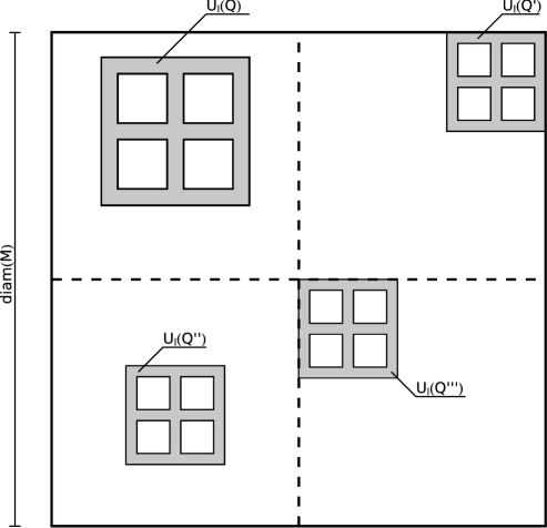
Figure 3. The ring domains (shaded) $U_{l}(Q)$, $U_{l}(Q^{\prime})$, $U_{l}(Q^{\prime\prime})$, $U_{l}(Q^{\prime\prime\prime})$ contained in sets of constancy of the Haar function $h_{M}$ (bold continous and dashed lines).

At first we parametrize the double series according to $\lambda$, where $\operatorname{diam}(Q)=2^{-\lambda}\,\operatorname{diam}(M)$,

$$A_{l}u =\sum_{\lambda=0}^{\infty}\sum_{\begin{subarray}{c}Q,M\in\mathscr{Q}:\\ \operatorname{sl}(Q)=2^{-\lambda}\operatorname{sl}(M)\end{subarray}}\langle f_{Q,l},h_{M}\rangle\,h_{Q}\,u_{M}\,|Q|^{-1}|M|^{-1}$$

$$=\sum_{\lambda=0}^{\infty}A_{l,\lambda}\,u.$$

Observe that with the ratio

$$\operatorname{diam}(Q)=2^{-\lambda}\,\operatorname{diam}(M)$$

fixed and recalling definition (3.2) we have

$$\{Q\,:\,\langle f_{Q,l},h_{M}\rangle\neq 0\}\subset\{Q\,:\,Q\cap D_{\lambda}(M)\neq\emptyset\}=\cal U_{\lambda}(M).$$

Using this fact one has the identity

$$A_{l,\lambda}\,u=\sum_{M\in\mathscr{Q}}u_{M}\,|M|^{-1}\sum_{Q\in\cal U_{\lambda}(M)}\langle f_{Q,l},h_{M}\rangle\,|Q|^{-1}\,h_{Q},$$

hence glancing at (4.17), utilizing the $\mathrm{UMD}$–property and Kahane’s contraction principle, we obtain

$$\|A_{l,\lambda}u\|_{L_{X}^{p}} \lesssim 2^{-l}\,\big{\|}\sum_{M\in\mathscr{Q}}u_{M}\,|M|^{-1}\sum_{Q\in\cal U_{\lambda}(M)}h_{Q}\big{\|}_{L_{X}^{p}}$$

$$=2^{-l}\,\big{\|}\sum_{M\in\mathscr{Q}}u_{M}\,g_{M,\lambda}\,|M|^{-1}\big{\|}_{L_{X}^{p}}.$$

Applying the triangle inequality, using the above estimate for $A_{l,\lambda}$, considering the definition of the ring domain operator (3.5), and invoking theorem 3.3 yields

$$\|A_{l}u\|_{L_{X}^{p}}\leq\sum_{\lambda=0}^{\infty}\|A_{l,\lambda}u\|_{L_{X}^{p}}\lesssim 2^{-l}\,\sum_{\lambda=0}^{\infty}\|S_{\lambda}u\|_{L_{X}^{p}}\lesssim 2^{-l}\,\sum_{\lambda=0}^{\infty}2^{-\lambda/\cal C(L_{X}^{p})}\,\|u\|_{L_{X}^{p}}.$$

Evaluating the geometric series we attain the estimate

$$\|A_{l}u\|_{L_{X}^{p}}\leq C\,2^{-l}\,\|u\|_{L_{X}^{p}},$$ (4.21)

where the constant $C$ depends on $n$, $p$, $X$ and $\cal C(L_{X}^{p})$.

Being aware that with $\lambda\geq 0$ fixed, the collections $\cal U_{\lambda}(M)$ are not disjoint as $M$ ranges over $\mathscr{Q}$ but the overlap is bounded by a constant depending solely on the dimension $n$ and the constant appearing in the definition of $D_{\lambda}(Q)$, we could have partitioned $\mathscr{Q}$ in a constant number of sets, generically denoted by $\mathscr{B}\subset\mathscr{Q}$, such that the $\cal U_{\lambda}(M)$ would not have interfered with each other in the first place. Then one can repeat the argument above, with $\mathscr{Q}$ replaced by one of the collections $\mathscr{B}$.

Reduction for $B_{l}$

This setting is visualised in figure 4.

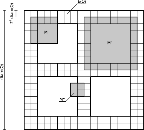
Figure 4. The cubes $M$, $M^{\prime}$ and $M^{\prime\prime}$ (shaded) intersecting the cubes $E(Q)$ of $\cal U_{l}(Q)$ (thin lines).

Note that the cubes $M$ are now smaller than $Q$, but bigger than the building blocks of the ring domain $\cal U_{l}(Q)$, so $2^{-l}\operatorname{diam}(Q)\leq\operatorname{diam}(M)<\operatorname{diam}(Q)$. We may use inequality (4.18) for estimating $\langle f_{Q,l},h_{M}\rangle$.

This time we prefer to analyze $B_{l}^{*}$, certainly with respect to the norm $\|\cdot\|_{L_{Y}^{q}}$, where $Y=X^{*}$ and $\frac{1}{p}+\frac{1}{q}=1$. As before we rearrange the series to see

$$B_{l}^{*}u =\sum_{\lambda=1}^{l}\sum_{\begin{subarray}{c}Q,M\in\mathscr{Q}:\\ \operatorname{sl}(M)=2^{-\lambda}\operatorname{sl}(Q)\end{subarray}}\langle f_{Q,l},h_{M}\rangle\,|M|^{-1}h_{M}\,u_{Q}\,|Q|^{-1}$$

$$=\sum_{\lambda=0}^{\infty}B_{l,\lambda}^{*}\,u.$$

When restricted to the fixed ratio

$$\operatorname{diam}(M)=2^{-\lambda}\,\operatorname{diam}(Q),$$

note that

$$\{M\,:\,\langle f_{Q,l},h_{M}\rangle\neq 0\}\subset\{M\,:\,M\cap D_{l}(Q)\neq\emptyset\}=\cal U_{\lambda}(Q),$$

so we can rewrite $B_{l,\lambda}^{*}u$ as follows:

$$B_{l,\lambda}^{*}u=\sum_{Q\in\mathscr{Q}}u_{Q}\,|Q|^{-1}\sum_{M\in\cal U_{\lambda}(Q)}\langle f_{Q,l},h_{M}\rangle\,|M|^{-1}h_{M}.$$

Taking the norm, utilizing the $\mathrm{UMD}$–property and applying Kahane’s contraction principle to (4.18) yields the estimate

$$\|B_{l,\lambda}^{*}u\|_{L_{Y}^{q}} \lesssim 2^{-l}\,\big{\|}\sum_{Q\in\mathscr{Q}}u_{Q}\,|Q|^{-1}\sum_{M\in\cal U_{\lambda}(Q)}h_{M}\big{\|}_{L_{Y}^{q}}$$

$$=2^{-l}\,\big{\|}\sum_{Q\in\mathscr{Q}}u_{Q}\,g_{Q,\lambda}|Q|^{-1}\big{\|}_{L_{Y}^{q}}.$$

In view of theorem 3.3 one proceeds

$$\|B_{l}^{*}u\|_{L_{Y}^{q}}\leq\sum_{\lambda=0}^{\infty}\|B_{l,\lambda}^{*}\,u\|_{L_{Y}^{q}}\lesssim 2^{-l}\sum_{\lambda=1}^{l}2^{\lambda}\,\big{\|}S_{\lambda}u\big{\|}_{L_{Y}^{q}}\lesssim 2^{-l}\sum_{\lambda=1}^{l}2^{\lambda(1-1/\cal C(L_{Y}^{q}))}\,\big{\|}u\big{\|}_{L_{Y}^{q}},$$

to conclude this case, retaining

$$\|B_{l}^{*}u\|_{L_{Y}^{q}}\leq C\,2^{-l/\cal C(L_{Y}^{q})}\big{\|}u\big{\|}_{L_{Y}^{q}},$$ (4.22)

where the constant $C$ depends on $n$, $q$ and $Y$.

Reduction for $C_{l}$

We may think of the cube $M$ being much smaller than $Q$, even smaller than the building blocks of the ring domain $\cal U_{l}(Q)$, and we have inequality (4.19) at our disposal. This is visualised in figure 5.

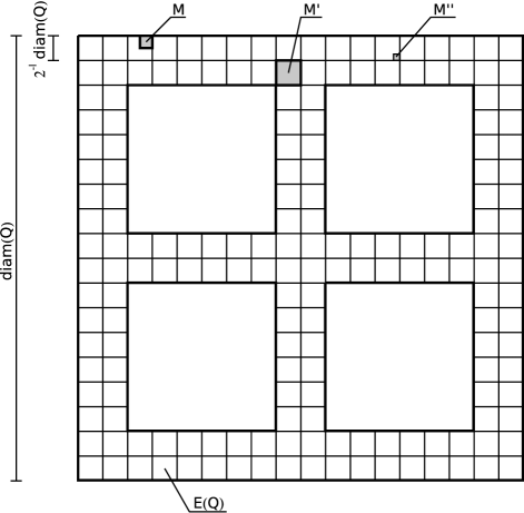
Figure 5. The cubes $M$, $M^{\prime}$ and $M^{\prime\prime}$ (shaded) contained in the cover $\cal U_{l}(Q)$ (thin lines).

As in the preceeding case we aim at estimating the adjoint operator $C_{l}^{*}$; so with $Y=X^{*}$ and $\frac{1}{p}+\frac{1}{q}=1$ the usual parametrization leads to

$$C_{l}^{*}u =\sum_{\lambda=l+1}^{\infty}\sum_{\begin{subarray}{c}Q,M\in\mathscr{Q}:\\ \operatorname{sl}(M)=2^{-\lambda}\operatorname{sl}(Q)\end{subarray}}\langle f_{Q,l},h_{M}\rangle\,|M|^{-1}h_{M}\,u_{Q}\,|Q|^{-1}$$

$$=\sum_{\lambda=l+1}^{\infty}C_{l,\lambda}^{*}u.$$

Under the restriction of $\operatorname{diam}(M)=2^{-\lambda}\,\operatorname{diam}(Q)$ holds that

$$\{M\,:\,\langle f_{Q,l},h_{M}\rangle\neq 0\}\subset\{M\,:\,M\cap D_{l}(Q)\neq\emptyset\}\approx\cal U_{l}(Q).$$

Note that the last equality is not true algebraically, indicated by ”$\approx$”. This notation is justified by the $\mathrm{UMD}$–property and Kahane’s contraction principle, which enables us to exchange zero mean Haar functions, as long as their supports are preserved.

We proceed by applying essentially the same steps as supplied before, now having estimate (4.19) at hand. Using the $\mathrm{UMD}$–property and Kahane’s contraction principle to (4.19) and

$$\big{|}\sum_{\begin{subarray}{c}M\in\mathscr{Q}\,:\,M\cap D_{l}(Q)\neq\emptyset\\ \operatorname{sl}(M)=2^{-\lambda}\operatorname{sl}(Q)\end{subarray}}h_{M}\big{|}\leq\big{|}\sum_{M\in\cal U_{l}(Q)}h_{M}\big{|}=|g_{Q,l}|,$$

we gain

$$\|C_{l,\lambda}^{*}u\|_{L_{Y}^{q}}\lesssim 2^{l}\,2^{-\lambda}\big{\|}\sum_{Q\in\mathscr{Q}}u_{Q}\,g_{Q,l}\,|Q|^{-1}\big{\|}_{L_{Y}^{q}},$$

thus, the triangle inequality and the above estimate for $C_{l,\lambda}^{*}$ yield

$$\|C_{l}^{*}u\|_{L_{Y}^{q}}\lesssim\big{\|}S_{l}u\big{\|}_{L_{Y}^{q}}.$$

Finally, theorem 3.3 yields

$$\|C_{l}^{*}u\|_{L_{Y}^{q}}\leq C\,2^{-l/\cal C(L_{Y}^{q})},$$ (4.23)

where the constant $C$ depends only on $n$, $q$ and $Y$.

Summary

We combine the inequalities (4.21), (4.22), (4.23), exploit that for $Y=X^{*}$ and $\frac{1}{p}+\frac{1}{q}=1$ holds

$$(L_{X}^{p})^{*}=L_{Y}^{q}\qquad\text{and}\qquad\frac{1}{\cal T(L_{X}^{p})}+\frac{1}{\cal(L_{Y}^{q})}=1,$$

to obtain

$$\|P_{l}\,:\,L_{X}^{p}\rightarrow L_{X}^{p}\|\leq C\,2^{-l(1-\frac{1}{\cal T(L_{X}^{p})})},$$ (4.24)

where $L_{X}^{p}$ has type $\cal T(L_{X}^{p})$ and the constant $C$ depends only on $n$, $p$, $X$, particularly on $\cal T(L_{X}^{p})$ and $\cal C(L_{X}^{p})$.

Very seperate reasons, that was the special shape of the support of $f_{Q,l}$ on the one hand, and the constancy of the Haar function $h_{M}$ exploiting the zero mean of $f_{Q,l}$ on the other hand, enabled us to reduce the estimates for $P_{l}$ to ring domain operators

$$S_{\lambda}u=\sum_{Q\in\mathscr{Q}}u_{Q}\,g_{Q,\lambda}\,|Q|^{-1},$$

where

$$g_{Q,\lambda}=\sum_{E\in\cal U_{\lambda}(Q)}h_{E},\qquad\text{and}\qquad u=\sum_{Q\in\mathscr{Q}}u_{Q}\,h_{Q}\,|Q|^{-1}.$$

4.3.2. Estimates for $P_{l}^{(\varepsilon)}$, $l<0$

We want to find estimates for the remaining sum

$$P_{-}=\sum_{l<0}P_{l}.$$

The argument is analogously to the case $l\geq 0$ completed in 4.3.1. The splitting of $\mathscr{Q}\times\mathscr{Q}$ will be according to the behaviour of $\langle f_{Q},h_{M}\rangle$ in (4.27) and (4.28), inducing the decomposition of $P_{-}$. The functions $f_{Q}$ are defined beneath.

Dropping all superscripts we issue representation (4.9) 4.9 for the kernel of $P_{l}$

$$K_{l}(x,y)=\sum_{Q\in\mathscr{Q}}h_{Q}(x)\,f_{Q,l}(y)\,|Q|^{-1},$$

and recall that for $Q\in\mathscr{Q}_{j}$

$$f_{Q,l}=\Delta_{j+l}h_{Q}=h_{Q}*d_{j+l}=h_{Q}*(b_{j+l+1}-b_{j+l}).$$

Taking the sum over $l<0$ yields

$$\sum_{l<0}f_{Q,l}=h_{Q}*d_{j}$$

since $\lim_{l\rightarrow\infty}b_{j+l}\xrightarrow{\text{p.w.}}0$, and so we define the mollified Haar functions

$$f_{Q}=h_{Q}*d_{j},\qquad\text{for all $Q\in\mathscr{Q}_{j}$}.$$

For the properties of the mollifier $d_{j}$ one might want to take a look at (4.3) and (4.4).

In this way we obtain the kernel $K_{-}(x,y)$ of the operator $P_{-}$

$$K_{-}(x,y)=\sum_{l<0}K_{l}(x,y)=\sum_{Q\in\mathscr{Q}}h_{Q}(x)\,f_{Q}(y)\,|Q|^{-1}.$$

In (4.12) 4.12 we observed that for $l=0$ there exists a $C>0$ so that for $Q\in\mathscr{Q}$

$$\int_{\ }f_{Q}(x)\,dx =0, \operatorname{supp}f_{Q} \subset C\cdot Q,$$ (4.25)

$$|f_{Q}| \leq C, \mathrm{Lip}(f_{Q}) \leq C\,(\operatorname{diam}(Q))^{-1}.$$

Figiel’s expansion, the $\mathrm{UMD}$–property and Kahane’s contraction principle yields the following generic form of the kernel

$$K_{-}(x,y)=\sum_{M,Q\in\mathscr{Q}}\langle f_{Q},h_{M}\rangle\,|M|^{-1}|Q|^{-1}h_{Q}(x)\,h_{M}(y).$$ (4.26)

Again, we need to analyze the properties of the coefficients $\langle f_{Q},h_{M}\rangle$. As in the preceeding cases, the estimates strongly depend on the ratio of the diameters of $Q$ and $M$.

1. If $\operatorname{diam}(M)\leq\operatorname{diam}(Q)$, we make use of

   $$\mathrm{Lip}(f_{Q})\leq C\,(\operatorname{diam}(Q))^{-1},$$

   according to (4.25) and discover

   $$|\langle f_{Q},h_{M}\rangle|\lesssim(\operatorname{diam}(Q))^{-1}\,(\operatorname{diam}(M))^{n+1},$$ (4.27)

2. while if $\operatorname{diam}(M)>\operatorname{diam}(Q)$, one can exploit

   $$|f_{Q}|\leq C\qquad\text{and}\qquad\operatorname{supp}f_{Q}\subset C\cdot Q$$

   to obtain

   $$|\langle f_{Q},h_{M}\rangle|\lesssim|Q|.$$ (4.28)

The coefficient $\langle f_{Q},h_{M}\rangle$ vanishes if the support of $f_{Q}$ is contained in a set where $h_{M}$ is constant. Precisely, let $\{M_{i}\}_{1\leq i\leq 2^{n}}$ be the immediate dyadic successors of $M$, then if

$$\operatorname{supp}f_{Q}\subset M_{i},$$

for an $1\leq i\leq 2^{n}$, we have

$$\langle f_{Q},h_{M}\rangle=0.$$

Hence, for $\operatorname{diam}(M)>\operatorname{diam}(Q)$ the cubes $Q$ for which $\langle f_{Q},h_{M}\rangle\neq 0$ cluster in the vicinity of $D(M)$, the set of $h_{M}$’s discontinuities.

We start the analysis of the Operators $P_{-}$ using the representation (4.26), that is

$$\big{(}P_{-}u\big{)}(x) =\int_{\ }K_{-}(x,y)\,u(y)\,dy,$$

and

$$K_{-}(x,y) =\sum_{Q,M\in\mathscr{Q}}\langle f_{Q},h_{M}\rangle\,h_{Q}(x)\,h_{M}(y)\,|Q|^{-1}|M|^{-1}.$$

Driven by (4.27) and (4.28), we split the set of all pairs of dyadic cubes $\mathscr{Q}\times\mathscr{Q}$ in

$$\cal A_{-} =\big{\{}(Q,M)\,:\,\operatorname{diam}(M)\leq\operatorname{diam}(Q)\big{\}},$$

$$\cal B_{-} =\big{\{}(Q,M)\,:\,\operatorname{diam}(M)>\operatorname{diam}(Q)\big{\}},$$

and define the associated kernels

$$A_{-}(x,y) =\sum_{(Q,M)\in\cal A_{-}}\langle f_{Q},h_{M}\rangle\,h_{Q}(x)\,h_{M}(y)\,|Q|^{-1}|M|^{-1},$$

$$B_{-}(x,y) =\sum_{(Q,M)\in\cal B_{-}}\langle f_{Q},h_{M}\rangle\,h_{Q}(x)\,h_{M}(y)\,|Q|^{-1}|M|^{-1},$$

accordingly.

Estimates for $A_{-}$

In this case the size of cube $M$ cannot exceed that of $Q$, so we may use inequality (4.27). We rather want to estimate $A_{-}^{*}$ than $A_{-}$ itself, therefore $Y=X^{*}$ and $\frac{1}{p}+\frac{1}{q}=1$. Rearranging the series in $A_{-}^{*}$ according to the ratio of the diameters of $Q$ and $M$ yields

$$A_{-}^{*}u =\sum_{\lambda=0}^{\infty}\sum_{\begin{subarray}{c}Q,M\in\mathscr{Q}:\\ \operatorname{sl}(M)=2^{-\lambda}\operatorname{sl}(Q)\end{subarray}}\langle f_{Q},h_{M}\rangle\,u_{Q}\,|Q|^{-1}h_{M}\,|M|^{-1}$$

$$=\sum_{\lambda=0}^{\infty}A_{-,\lambda}^{*}u.$$

Taking the norm and applying the triangle inequality to the first sum

$$\|A_{-}^{*}u\|_{L_{Y}^{q}}\leq\sum_{\lambda=0}^{\infty}\big{\|}A_{-,\lambda}^{*}u\|_{L_{Y}^{q}},$$

necessitates to estimate $A_{-,\lambda}^{*}$. Utilizing the $\mathrm{UMD}$–property and Kahane’s contraction principle (2.5) applied to (4.27), we infer

$$\big{\|}A_{-,\lambda}^{*}u\big{\|}_{L_{Y}^{q}}\lesssim 2^{-\lambda}\big{\|}\sum_{Q\in\mathscr{Q}}\sum_{\begin{subarray}{c}\operatorname{sl}(M)=2^{-\lambda}\operatorname{sl}(Q)\\ M\cap(C\cdot Q)\neq\emptyset\end{subarray}}u_{Q}\,|Q|^{-1}h_{M}\big{\|}_{L_{Y}^{q}}.$$

For every $Q\in\mathscr{Q}$ we issue Kahane’s contraction principle on

$$\big{|}\sum_{\begin{subarray}{c}\operatorname{sl}(M)=2^{-\lambda}\operatorname{sl}(Q)\\ M\cap(C\cdot Q)\neq\emptyset\end{subarray}}h_{M}\big{|}\leq|h_{Q}|,$$

keeping in mind that we would actually need a constant number of Figiel shifts of $h_{Q}$ to cover the whole support of this sum. Nevertheless, the bound (2.9) allows us to estimate

$$\big{\|}A_{-,\lambda}^{*}u\big{\|}_{L_{Y}^{q}} \lesssim 2^{-\lambda}\,\big{\|}\sum_{Q\in\mathscr{Q}}u_{Q}\,|Q|^{-1}\sum_{\begin{subarray}{c}\operatorname{sl}(M)=2^{-\lambda}\operatorname{sl}(Q)\\ M\cap(C\cdot Q)\neq\emptyset\end{subarray}}h_{M}\big{\|}_{L_{Y}^{q}}$$

$$\lesssim 2^{-\lambda}\,\big{\|}u\big{\|}_{L_{Y}^{q}}.$$

To conclude, we string together our estimates, yielding

$$\|A_{-}^{*}u\|_{L_{X}^{p}}\leq C\,\|u\|_{L_{X}^{p}},$$ (4.29)

where the constant $C$ depends on $n$, $q$ and $Y$.

Estimates for $B_{-}$

In this setting the size of $M$ does exceed $Q$.

With the usual parametrization of $B_{-}$ we have

$$B_{-}u =\sum_{\lambda=1}^{\infty}\sum_{\begin{subarray}{c}Q,M\in\mathscr{Q}:\\ \operatorname{diam}(Q)=2^{-\lambda}\operatorname{diam}(M)\end{subarray}}\langle f_{Q},h_{M}\rangle\,h_{Q}\,|Q|^{-1}u_{M}\,|M|^{-1}$$

$$=\sum_{\lambda=1}^{\infty}B_{-,\lambda}u.$$

Restricted to cubes $Q,M\in\mathscr{Q}$ with

$$2^{-\lambda}\operatorname{diam}(M)=\operatorname{diam}(Q)$$

one can see that for all $M$ the following holds true:

$$\{Q\,:\,\langle f_{Q},h_{M}\rangle\neq 0\}\subset\{Q\,:\,(C\cdot Q)\cap D(Q)\neq\emptyset\}\subset\cal U_{\lambda}(M).$$

Successively using the $\mathrm{UMD}$–property, Kahane’s contraction principle applied to (4.28) and the inclusion above we obtain

$$\big{\|}B_{-,\lambda}u\big{\|}_{L_{X}^{p}} \lesssim\big{\|}\sum_{M\in\mathscr{Q}}u_{M}\,|M|^{-1}\,\sum_{Q\in\cal U_{\lambda}(M)}h_{Q}\big{\|}_{L_{X}^{p}}$$

$$=\big{\|}\sum_{M\in\mathscr{Q}}u_{M}\,g_{M,\lambda}\,|M|^{-1}\big{\|}_{L_{X}^{p}}.$$

The main result on ring domain operators theorem 3.3 yields

$$\|B_{-,\lambda}u\|_{L_{X}^{p}}\lesssim\|S_{\lambda}u\|_{L_{X}^{p}}\lesssim 2^{-\lambda/\cal C(L_{X}^{p})}\,\|u\|_{L_{X}^{p}},$$

hence merging our inequalities we attain

$$\|B_{-}u\|_{L_{X}^{p}}\leq C\,\|u\|_{L_{X}^{p}},$$ (4.30)

where the constant $C$ depends on $n$, $p$, $X$ and $\cal C(L_{X}^{p})$.

Summary

Inequality (4.29) and (4.30) together imply the boundedness for the mollified operator $P_{-}$

$$\|P_{-}\,:\,L_{X}^{p}\rightarrow L_{X}^{p}\|\leq C,$$ (4.31)

where the constant $C$ depends on $n$, $p$, $X$, particularly on $\cal T(L_{X}^{p})$ and $\cal C(L_{X}^{p})$.

In the case $l\leq 0$, the shape of the support of the mollified Haar function $f_{Q,l}$ is not a ring domain, opposed to the case $l\geq 0$. So we cannot expect to reduce our estimates to ring domain operators in cases where the shape of the support of $f_{Q,l}$ is crucial. Revisiting the reduction to ring domain operators for $l\geq 0$, it is clear that the reduction to ring domain operators is feasible for the operator $B_{-}$, since we can still exploit the zero mean of $f_{Q,l}$ on sets where $h_{M}$ is constant.

4.4. Estimates for $P_{l}^{(\varepsilon)}R_{i_{0}}^{-1}$

In this brief section we will establish estimates for $P_{l}^{(\varepsilon)}R_{i_{0}}^{-1}$, $l\in\mathbb{Z}$ by reducing them to estimates for $P_{l}^{(\varepsilon)}$. This necessitates that $\big{(}R_{i_{0}}^{-1}\big{)}^{*}$ maps the mollified Haar functions $f_{Q,l}^{(\varepsilon)}$ to functions $k_{Q,l}^{(\varepsilon)}$ enjoying similar properties. Due to the algebraic identity (4.32), this amounts to controlling the support of the $k_{Q,l}$ (besides factors depending on $l$). Assuming $\varepsilon_{i_{0}}=1$, one can exploit

$$\operatorname{supp}\big{(}\operatorname{\mathbb{E}}_{i_{0}}h_{Q}^{(\varepsilon)}\big{)}\subset Q,$$

provoking the functions $k_{Q,l,i}$ defined in (4.33) to exhibit the support conditions asserted in (4.34) and (4.35).

It is a well known fact that one can write the inverse of the Riesz transform as

$$R_{i_{0}}^{-1}=R_{i_{0}}+\sum_{\begin{subarray}{c}1\leq i\leq n\\ i\neq i_{0}\end{subarray}}\mathbb{E}_{i_{0}}\partial_{i}R_{i},$$ (4.32)

where $\mathbb{E}_{i_{0}}$ denotes integration with respect to the $i_{0}$–th variable,

$$\mathbb{E}_{i_{0}}f(x)=\int_{-\infty}^{x_{i_{0}}}f(x_{1},\ldots,x_{i_{0}-1},s,x_{i_{0}+1},\ldots,x_{n})\,\mathrm{d}s,\qquad x=(x_{1},\ldots,x_{n}).$$

Now we introduce the family of functions

$$k_{Q,l,i}^{(\varepsilon)}=\Delta_{j+l}\big{(}\mathbb{E}_{i_{0}}\partial_{i}h_{Q}^{(\varepsilon)}\big{)},\qquad\text{if $Q\in\mathscr{Q}_{j}$},$$ (4.33)

and consider

$$P_{l}^{(\varepsilon)}R_{i_{0}}^{-1}u =\sum_{j\in\mathbb{Z}}\sum_{Q\in\mathscr{Q}_{j}}\big{\langle}R_{i_{0}}u,\Delta_{j+l}(h_{Q}^{(\varepsilon)})\big{\rangle}\,h_{Q}^{(\varepsilon)}\,|Q|^{-1}$$

$$\quad+\sum_{\begin{subarray}{c}1\leq i\leq n\\ i\neq i_{0}\end{subarray}}\sum_{j\in\mathbb{Z}}\sum_{Q\in\mathscr{Q}_{j}}\big{\langle}\mathbb{E}_{i_{0}}\partial_{i}R_{i}u,\Delta_{j+l}(h_{Q}^{(\varepsilon)})\big{\rangle}\,h_{Q}^{(\varepsilon)}\,|Q|^{-1}.$$

Since the Riesz transforms are continous mappings, it is obvious that the first sum can be treated as in section 4.3. For the seond sum, we fix a coordinate $i\neq i_{0}$, rearrange the operators in the scalar product and use the functions defined in (4.33), hence

$$\sum_{j\in\mathbb{Z}}\sum_{Q\in\mathscr{Q}_{j}}\langle\mathbb{E}_{i_{0}}\partial_{i}R_{i}u,\Delta_{j+l}(h_{Q}^{(\varepsilon)})\rangle\,h_{Q}^{(\varepsilon)}\,|Q|^{-1}=\sum_{Q\in\mathscr{Q}}\langle R_{i}u,k_{Q,l,i}^{(\varepsilon)}\rangle\,h_{Q}^{(\varepsilon)}\,|Q|^{-1}.$$

The continuity of the Riesz transforms $R_{i}:L_{X}^{p}\rightarrow L_{X}^{p}$ allows us to estimate the following simpler type of operator

$$K_{l,i}^{(\varepsilon)}u=\sum_{Q\in\mathscr{Q}}\langle u,k_{Q,l,i}^{(\varepsilon)}\rangle\,h_{Q}^{(\varepsilon)}\,|Q|^{-1}.$$

In order to estimate $K_{l,i}^{(\varepsilon)}$ we need to analyze the analytic properties of the functions $k_{Q,l,i}^{(\varepsilon)}$. If $l\geq 0$, then

$$\int_{\ }k_{Q,l,i}^{(\varepsilon)}(x)\,dx =0, \operatorname{supp}k_{Q,l,i}^{(\varepsilon)} \subset D_{l}^{(\varepsilon)}(Q),$$ (4.34)

$$|k_{Q,l,i}^{(\varepsilon)}| \leq C\,2^{l}, \mathrm{Lip}(k_{Q,l,i}^{(\varepsilon)}) \leq C\,2^{2l}\,(\operatorname{diam}(Q))^{-1},$$

and for $l\leq 0$

$$\int_{\ }k_{Q,l,i}^{(\varepsilon)}(x)\,dx =0, \operatorname{supp}k_{Q,l,i}^{(\varepsilon)} \subset C\,2^{|l|}Q,$$ (4.35)

$$|k_{Q,l,i}^{(\varepsilon)}| \leq C\,2^{-|l|(n+1)}, \mathrm{Lip}(k_{Q,l,i}^{(\varepsilon)}) \leq C\,2^{-|l|(n+2)}\,(\operatorname{diam}(Q))^{-1}.$$

Note that the above properties of $k_{Q,l,i}^{(\varepsilon)}$ especially depend on the coordinatewise vanishing moments of $b$ (4.3), introduced by $\Delta_{l}$ in equations (4.4) and (4.6). Furthermore observe the definition of $k_{Q,l,i}^{(\varepsilon)}$ involves an integration of $h_{Q}^{(\varepsilon)}$ with respect to the variable $x_{i_{0}}$. Now if $\varepsilon_{i_{0}}=1$, then $\operatorname{\mathbb{E}}_{i_{0}}h_{Q}^{(\varepsilon)}$ is compactly supported in $Q$, but if $\varepsilon_{i_{0}}=0$, then $\operatorname{supp}\big{(}\operatorname{\mathbb{E}}_{i_{0}}h_{Q}^{(\varepsilon)}\big{)}$ is unbounded. This urges the dominating Riesz transform $R_{i_{0}}$ to act on a coordinate $x_{i_{0}}$ for which $P^{(\varepsilon)}$ projects onto zero mean Haar functions, thus necessitating $\varepsilon_{i_{0}}=1$.

If we compare this with the properties (4.12) and (4.13) regarding the functions $f_{Q,l}^{(\varepsilon)}$, it turns out that the properties coincide if $l\leq 0$, and that $2^{-l}\,k_{Q,l,i}^{(\varepsilon)}$, satisfies the same conditions as $f_{Q,l}^{(\varepsilon)}$, if $l\geq 0$. Bootstrapping the proofs in section 4.3, we note that those arguments where solely depending on the analytic properties (4.12) and (4.13) of the functions $f_{Q,l}^{(\varepsilon)}$. With regard to (4.34) respectively (4.34), the same proofs are practicable with the functions $k_{Q,l,i}^{(\varepsilon)}$, if $l\leq 0$, respectively $2^{-l}\,k_{Q,l,i}^{(\varepsilon)}$, if $l\geq 0$, replacing $f_{Q,l}$. Stringing this all together implies the following upper bounds for the operators $K_{l,i}^{(\varepsilon)}$ and $K_{-,i}^{(\varepsilon)}$, where

$$K_{-,i}^{(\varepsilon)}=\sum_{l\leq 0}K_{l,i}^{(\varepsilon)}.$$

Estimate (4.31) implies

$$\|K_{-,i}^{(\varepsilon)}\,:\,L_{X}^{p}\rightarrow L_{X}^{p}\|\leq C,$$

and if $l\geq 0$, then using estimate (4.14) on $2^{-l}\,K_{l,i}^{(\varepsilon)}$ yields

$$\|K_{l,i}^{(\varepsilon)}\,:\,L_{X}^{p}\rightarrow L_{X}^{p}\|\leq C\,2^{l/\cal T(L_{X}^{p})},$$

where the constant $C$ depends on $n$, $p$, $X$, particularly on $\cal T(L_{X}^{p})$ and $\cal C(L_{X}^{p})$.

Obviously, the estimate for the operators $P_{l}^{(\varepsilon)}R_{i_{0}}^{-1}$ ist just a constant multiple of the operator norm of $K_{l,i}^{(\varepsilon)}$, so we summarize:

If $\varepsilon_{i_{0}}=1$, then the following inequalities hold true:

$$\|P_{-}^{(\varepsilon)}R_{i_{0}}^{-1}\,:\,L_{X}^{p}\rightarrow L_{X}^{p}\|\leq C,$$ (4.36)

and for all $$l\geq 0$$

$$\|P_{l}^{(\varepsilon)}R_{i_{0}}^{-1}\,:\,L_{X}^{p}\rightarrow L_{X}^{p}\|\leq C\,2^{l/\cal T(L_{X}^{p})},$$ (4.37)

where the constant $C$ depends merely on $n$, $p$, $X$, $\cal T(L_{X}^{p})$ and $\cal C(L_{X}^{p})$.

References

- [BS88] C. Bennett and R. Sharpley. Interpolation of Operators. Academic Press, 1988.
- [Bur81] D. L. Burkholder. A Geometrical Characterization of Banach Spaces in which Martingale Difference Sequences are Unconditional. Annals of Probability, 9(6):997–1011, 1981.
- [Bur86] D. L. Burkholder. Martingales and Fourier Analysis in Banach Spaces. In Lecture Notes in Mathematics, volume 1206, pages 61–108. Springer, 1986.
- [Fig88] T. Figiel. On Equivalence of Some Bases to the Haar System in Spaces of Vector-valued Functions. Bulletin of the Polish Academy of Sciences, 36(3–4):119–131, 1988.
- [Fig91] T. Figiel. Singular Integral Operators: A Martingale Approach. In Geometry of Banach Spaces, number 158 in London Mathematical Society Lecture Note Series, pages 95–110, 1991.
- [FM99] I. Fonseca and S. Müller. -quasiconvexity, lower semicontinuity, and Young measures. SIAM J. Math. Anal., 30(6):1355–1390, 1999.
- [LMM07] J. Lee, P. F. X. Mueller, and S. Mueller. Compensated Compactness, Separately Convex Functions and Interpolatory Estimates Between Riesz Transforms and Haar Projections. http://www.mis.mpg.de/preprints/2008/preprint2008_7.pdf, 2007.
- [MS86] V. D. Milman and G. Schechtman. Asymptotic Theory of Finite Dimensional Normed Spaces. Springer, 1986.
- [Mue99] S. Mueller. Rank-one Convexity Implies Quasiconvexity on Diagonal Matrices. International Mathematics Research Notices, 1999(20):1087–1095, 1999.
- [Mue05] P. F. X. Mueller. Isomorphisms Between Spaces. Birkhäuser, 2005.
- [Mur78] F. Murat. Compacite par compensation. Ann. Scuola Norm. Sup. Pisa, Cl. Sci. (4), 5(3):489–507, 1978.
- [Mur79] F. Murat. Compacite par compensation II. Recent methods in non-linear analysis, Proc. int. Meet., Rome 1978, 245-256, 1979.
- [Mur81] F. Murat. Compacite par compensation: condition necessaire et suffisante de continuite faible sous une hypothèse de rang constant. Ann. Scuola Norm. Sup. Pisa, Cl. Sci. (4), 8:69–102, 1981.
- [Ste70] E. M. Stein. Singular Integrals and Differentiability Properties of Functions. Princeton University Press, 1970.
- [Ste93] E. M. Stein. Harmonic Analysis: Real–Variable Methods, Orthogonality and Oscillatory Integrals. Princeton University Press, 1993.
- [Tar78] L. Tartar. Une nouvelle méthode de résolution d’équations aux dérivées partielles non linéaires. In Lecture Notes in Mathematics, volume 665, pages 228–241. Springer, 1978.
- [Tar79] L. Tartar. Compensated compactness and applications to partial differential equations. In Res. Notes Math., volume 39, pages 136–212. Pitman, 1979.
- [Tar83] L. Tartar. The compensated compactness method applied to systems of conservation laws. Systems of nonlinear partial differential equations, Proc. NATO Adv. Study Inst., Oxford/U.K. 1982, NATO ASI Ser. Ser., C 111, 263-285, 1983.
- [Tar84] L. Tartar. Étude des oscillations dans les équations aux dérivées partielles non linéaires. (Study of oscillations in nonlinear partial differential equations). Trends and applications of pure mathematics to mechanics, Symp., Palaiseau/France 1983, Lect. Notes Phys. 195, 384-412, 1984.
- [Tar90] L. Tartar. -measures, a new approach for studying homogenisation, oscillations and concentration effects in partial differential equations. Proc. R. Soc. Edinb., Sect. A, 115(3-4):193–230, 1990.
- [Tar92] L. Tartar. On mathematical tools for studying partial differential equations of continuum physics: -measures and Young measures. Buttazzo, Giuseppe (ed.) et al., Developments in partial differential equations and applications to mathematical physics. Proceedings of an international meeting, Ferrara, Italy, October 14-18, 1991. New York, NY: Plenum Press. 201-217, 1992.
- [Tar93] L. Tartar. Some remarks on separately convex functions. Kinderlehrer, David (ed.) et al., Microstructure and phase transition. Based on the proceedings of a workshop which was an integral part of the 1990-91 IMA program on phase transitions and free boundaries. New York, NY: Springer-Verlag. IMA Vol. Math. Appl. 54, 191-204, 1993.
- [Woj91] P. Wojtaszczyk. Banach Spaces for Analysts. Cambridge University Press, 1991.