Is thermo-ionic emission at room temperature exploitable?

Abstract

In this brief note we describe two devices, a sort of flat and spherical capacitor, with which one should be able to test the possibility of creating a macroscopic voltage, and thus exploitable current, out of a single thermal source at room temperature. The basic idea is trivial and it makes use of a thermo-emitting cathode with work function as low as $0.7\,$eV. The idea is not completely new, but our approach is simpler and neat. When implemented, it should allow to assess if approaches based on thermo-ionic materials at room temperature really violate the Second Law of Thermodynamics macroscopically.

Keywords: Thermo-ionic emission – Room temperature – Second Law of thermodynamics.

1 Introduction

The Second Law of Thermodynamics, explicitly in the form of Kelvin postulate, puts a fundamental limit to the way in which usable work can be extracted form heat sources, and to the maximum amount of work extractable (Carnot’s principle). In particular, Kelvin postulate states that it is not possible to cyclically extract work from a single heat source. Clausius postulate of the Second Law, which is notoriously equivalent to Kelvin postulate, makes the impossibility more striking and understandable: heat can not spontaneously flow from sources at absolute temperature $T_{1}$ to sources at absolute temperature $T_{2}$ if $T_{2}\geq T_{1}$.

Although in the macroscopic physical world the Second Law seems authoritatively to make the difference between what is allowed and what is forbidden, in the microscopic world it seems to be continuously violated: let’s take the Brownian motion or every fluctuation phenomena, for example.

As stated by Poincaré about Brownian motion [1]:

“[..]we see under our eyes now motion transformed into heat by friction, now heat changed inversely into motion, and that without loss since the movement lasts forever. This is contrary to the principle of Carnot.”.

Almost every past attempt to understand and exploit such microscopic violation relies in the approach of fluctuations rectification. Even the famous thought experiment of Maxwell’s Demon is based, in the end, on a idealized version of fluctuations rectification. The main difficulties with these approaches are that every macroscopic/microscopic rectifier device seems either to suffer fluctuations itself, which neutralize every usable net effect, or its functioning seems to increase the total entropy of the system, at least of the same amount of the alleged reduction, mainly because of energy dissipation and/or entropy cost in the acquisition of information needed to run the device. For a thorough historical account, see Earman and Norton [2].

An approach to microscopic rectification that seems theoretically promising is the equivalent of the photo-electric effect with materials emitting electrons at room temperature. If we are able to collect even a fraction of the electrons emitted by these materials due to the absorption of radiation by a single heat source, then we would be able in principle to transform their flow into work and heat again, indefinitely. As a matter of fact, if photo-voltaic cells exist, why, in principle, thermo-voltaic cells should not exist? As we will explain later in details, our approach appears not to suffer from the usual limitations [2].

Nowadays thermo-ionic materials are available that have a non negligible electronic emission at room temperature. For example, the well known Ag–O–Cs photo-cathode has a low work function, $\phi\lesssim 0.7\,$eV, and a peak emission at about $\lambda=8500$ Å [3, 4, 5].

Other researchers have tried to experimentally implement similar ideas in the past (see, for example, [6], [7, 8] and references therein). Unfortunately, their results, some of which have been published in peer-reviewed journals, have not received the attention they deserve from the scientific community.

As a matter of fact, those approaches share a common weakness: the current or the voltage produced are very small (microscopic in some cases) and, due to the complexity of the experimental apparatus (including the measurement equipment) and the complexity of the experimental conditions, it is often not possible to unambiguously decouple such a production from other sources known but not accounted for (magnetic fields, ordinary solid state and plasma physics effects, and so on).

In this note we provide a very simple and neat approach to test the exploitability of the ‘thermo-ionic emission idea’. In contrast with what has been previously done in our approach we do not need complex equipments, high temperatures, as in [6], or any external, constant and uniform (or not uniform) magnetic field as rectifier device, as in [7, 8]. In such a way we should eliminate possible sources of spurious and not controllable electric effect, due for example to known thermo-electric phenomena, to the measurement equipment and to external magnetic fields. Moreover, the simplicity of our approach allows us to mathematically model its behavior with a straightforward analysis: in this way a comparison between theory and experimental results could be carried out on a solid, quantitative ground.

In a few words, what we describe in the following Sections is an analogous of a thermo-voltaic cell.

2 Thermo-charged flat capacitor

Figure 1: Scheme of the thermo-charged flat capacitor.

In Fig. 1 a sketch of our first device is shown. It is substantially a flat capacitor with square plates of area $S$ and inter-plates distance $d$, with $\sqrt{S}\gg d$ in order to reduce boundary effects. The capacitor should be placed inside a case that is opaque to the visible light (in order to avoid spurious photo-electric emission), under extreme vacuum and at room temperature. The internal side of one of the plates is covered with a thin layer of Ag–O–Cs material.

Now, it should be clear how our device works. Almost half of the electrons emitted by the treated plate, due to thermo-ionic emission at room temperature, is collected by the second plate creating a macroscopic difference of potential $V$. Such process lasts until $V$ is too high to be overcome by the kinetic energy $K_{e}$ of the main fraction of emitted electrons (namely, when $K_{e}<eV$, where $e$ is the charge of electron). The other half of the emitted electrons, namely those emitted to the left in Fig. 1, remains confined in the metallic structure of the treated plate. The contact surface between the metallic plate and the Ag–O–Cs layer is a well known Schottky junction (metal/n-type semiconductor). When two materials (in our case, a metal and a semiconductor) are physically joined, so as to establish a uniform chemical potential, that is a single Fermi level, electrons are transferred from the material with the lesser work function $\phi_{1}$ (Ag–O–Cs) to the material with the greater work function $\phi_{2}$ (metal). As a result a contact potential $V_{c}$ is established such that $eV_{c}=\phi_{2}-\phi_{1}$. The energy band profiles of semiconductor-metal junction at equilibrium are shown in Fig. 2 a). The aspect which counts for the functioning of our device is the fact that the energy level of the vacuum for Ag–O–Cs (and that for the metallic plate) is preserved [9] far from the depletion region. This means that whenever an electron is extracted from the Ag–O–Cs to the vacuum (towards the second plate), and for what is said above this is made always at the cost of $\approx 0.7\,$eV, an electron must flow from the metallic plate to the Ag–O–Cs layer in order to re-establish the constant contact potential. Thus, the contact potential is not a wall which forbids every flux of electrons through the junction metal/Ag–O–Cs. Moreover, thermal photons with energy greater or equal to the energy gap between the Fermi level and the conduction region in the semiconductor generate the accumulation of electrons in the semiconductor side, creating a further thermo-voltage across the junction: and all this is due to the contact field in the depletion region of the junction (see Fig. 2 b)).

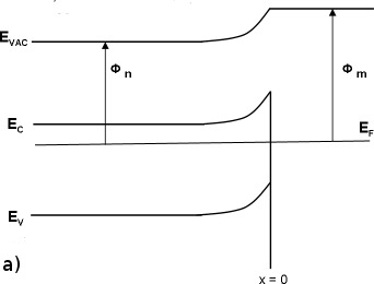
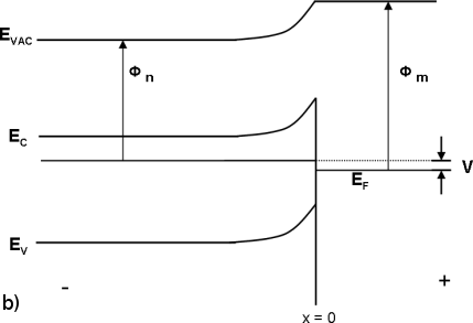
Figure 2: Figure a): Band profiles of semiconductor (n) - metal (m) junction at equilibrium. Figure b): Photo/thermo generated electrons accumulate in the n-type semiconductor. This rises the electron Fermi level and generates a further voltage $V$.

As it will be clear later in the text, it is important to reduce to zero the amount of electrons which escape from the treated plate and, due to the open sides, are not collected by the second metallic plate. In the long run such a dissipation could lead to an exhaustion of the charging process. As a matter of fact, the condition $\sqrt{S}\gg d$ has been chosen also to maximally reduce such undesired effect. This problem, anyway, could be completely fixed using closed, spherical capacitors, as we will see in Section 3.

If a resistor of suitable ohmic resistance is placed between the plates, then a macroscopic and potentially exploitable current should be measurable.

It could be interesting to provide an estimate of the value of $V$ obtainable and an estimate of the time needed to reach such value, given the physical characteristics of the capacitor and the quantum efficiency curve $\eta(\nu)$ of the thermo-ionic material.

The capacitor is placed in a heat bath at room temperature and it is subject to the black-body radiation. Every plate, at thermal equilibrium, emits and absorbs an equal amount of radiation (Kirchhoff’s law of thermal radiation), thus the amount of radiation absorbed by the thermo-ionic material is the same emitted by the plate according to the black-body radiation formula (Planck’s equation). Given the room temperature $T$, Planck equation provides us with the number distribution of photons absorbed as a function of their frequency.

According to the law of thermo-ionic emission, the kinetic energy $K_{e}$ of the electron emitted by the material is given by the following equation,

$$K_{e}=h\nu-\phi,$$ (1)

where $h\nu$ is the energy of the photon with frequency $\nu$ ($h$ is the Planck constant) and $\phi$ is the work function of the material. Thus, only the tail of the Planck distribution of photons absorbed, with frequency $\nu>\nu_{0}=\phi/h$, can contribute to the thermo-ionic emission.

The voltage $V$ reachable with frequency $\nu_{1}$ is given by the following formula,

$$eV=h\nu_{1}-\phi,$$ (2)

where $eV$ is the inter-plates potential energy, and thus,

$$\nu_{1}=\frac{eV+\phi}{h}.$$ (3)

The total number of photons per unit time $F_{p}$, with energy greater than or equal to $h\nu_{1}$, emitted and absorbed in thermal equilibrium by the internal side of treated plate is given by the Planck equation,

$$F_{p}=\frac{2\pi S}{c^{2}}\int_{\nu_{1}}^{\infty}\frac{\nu^{2}d\nu}{e^{\frac{h\nu}{kT}}-1},$$ (4)

where $S$ is the plate surface area, $c$ is the speed of light, $k$ is the Boltzmann constant and $T$ the room temperature.

If $\eta(\nu)$ is the quantum efficiency (or quantum yield) curve of the photo-cathode Ag–O–Cs, then the number of electrons per unit time $F_{e}$ with kinetic energy greater than or equal to $h\nu_{1}-\phi$ emitted (due to thermo-ionic effect) by the internal side of the treated plate towards the second metallic plate is given by,

$$F_{e}=\frac{2\pi S}{c^{2}}\int_{\nu_{1}}^{\infty}\frac{\eta(\nu)\nu^{2}d\nu}{e^{\frac{h\nu}{kT}}-1}.$$ (5)

As it is well known, the electric charge $Q$ of a flat capacitor is linked to the voltage as follows,

$$V=\frac{d}{\epsilon_{0}S}Q,$$ (6)

where $\epsilon_{0}$ is the dielectric constant of vacuum.

Now, we derive the differential equation which governs the process of thermo-charging. In the interval of time $dt$ the charge collected by the metallic plate is given by,

$$dQ=eF_{e}dt=\frac{2\pi eS}{c^{2}}\Biggl{(}\int_{\frac{eV(t)+\phi}{h}}^{\infty}\frac{\eta(\nu)\nu^{2}d\nu}{e^{\frac{h\nu}{kT}}-1}\Biggr{)}dt,$$ (7)

where we make use of eq. (3) for $\nu_{1}$ and $V(t)$ is the voltage at time $t$. Thus, through the differential form of eq. (6), we have,

$$dV(t)=\frac{2\pi ed}{\epsilon_{0}c^{2}}\Biggl{(}\int_{\frac{eV(t)+\phi}{h}}^{\infty}\frac{\eta(\nu)\nu^{2}d\nu}{e^{\frac{h\nu}{kT}}-1}\Biggr{)}dt,$$ (8)

or

$$\frac{dV(t)}{dt}=\frac{2\pi ed}{\epsilon_{0}c^{2}}\int_{\frac{eV(t)+\phi}{h}}^{\infty}\frac{\eta(\nu)\nu^{2}d\nu}{e^{\frac{h\nu}{kT}}-1}.$$ (9)

Unfortunately, provided that an analytical approximation of a real quantum efficiency curve $\eta(\nu)$ exists, the previous differential equation appears to have no general, simple analytical solution.

However, a close look at the Planckian integral of eq. (9) suggests us the asymptotic behavior of $V(t)$. Even if we do not know a priori how $\eta(\nu)$ is, we know it to be a bounded function of frequency, with values between zero and one; usually, the higher is $\nu$, the closer to $1$ is $\eta(\nu)$. Thus, independently from $\eta(\nu)$, a slight increase of $V(t)$ makes the value of the Planckian integral to be smaller and smaller very fast. Heuristically, this suggests that $V(t)$ should tend quite rapidly to an ‘asymptotic’ value (since $\frac{dV}{dt}$ tends to $0$).

In the rest of this section we provide a numerical solution of the above differential equation. To do so we need to adopt an approximation, however: the approximation we make consists in the adoption of a constant value for $\eta$, a sort of suitable mean value $\overline{\eta}$.

The differential equation (9) thus becomes,

$$\frac{dV(t)}{dt}=\frac{2\pi ed\overline{\eta}}{\epsilon_{0}c^{2}}\int_{\frac{eV(t)+\phi}{h}}^{\infty}\frac{\nu^{2}d\nu}{e^{\frac{h\nu}{kT}}-1}.$$ (10)

A straightforward variable substitution in the integral of eq. (10) allows us to write it in its final simplified form,

$$\frac{dV(t)}{dt}=\frac{2\pi ed\overline{\eta}}{\epsilon_{0}c^{2}}\biggl{(}\frac{kT}{h}\biggr{)}^{3}\int_{\frac{eV(t)+\phi}{kT}}^{\infty}\frac{x^{2}dx}{e^{x}-1}.$$ (11)

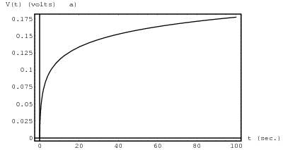
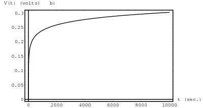
Figure 3: Thermo-charging process of the flat capacitor described in the text ($\phi=0.7\,$eV, $d=0.05\,$m, $T=298\,$K, and $\overline{\eta}=10^{-5}$). These two plots show with different ranges in time-scale the behavior of $V(t)$. Plot a) shows how only after 60 seconds the voltage of the capacitor becomes more than $0.15\,$volts. Instead, plot b) tells us that the voltage of the capacitor requires hundreds of hours to approach $0.3\,$volts.

Here we provide an exemplificative numerical solution of eq. (11), adopting the following nominal values for $\phi$, $d$, $T$ and $\overline{\eta}$: $\phi=0.7\,$eV, $d=0.05\,$m, $T=298\,$K, and $\overline{\eta}=10^{-5}$. In order to make a conservative choice for the value of $\overline{\eta}$ we note that only black body radiation with frequency greater than $\nu_{0}=\phi/h$ can contribute to the thermo-ionic emission. This means that for the Ag–O–Cs photo-cathode only radiation with wavelength smaller than $\lambda_{0}=hc/\phi\simeq 1700\,$nm contributes to the emission. According to Fig. 1 in Bates [5], the quantum yield of Ag–O–Cs for wavelengths smaller than $\lambda_{0}$ (and thus, for frequency greater than $\nu_{0}$) is always greater than $10^{-5}$. Anyway, a laboratory realization of the capacitor, together with the experimental measurement of $V(t)$, should provide us with a realistic estimate of $\overline{\eta}$ for the photo-cathode Ag–O–Cs.

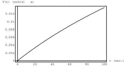
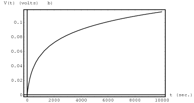
Figure 4: Thermo-charging process of the flat capacitor described in the text with $\phi=0.7\,$eV, $d=0.05\,$m, $T=298\,$K, and $\overline{\eta}=10^{-8}$. These two plots show with different ranges in time-scale the behavior of $V(t)$. Plot a) shows how only after 60 seconds the voltage of the capacitor is near to $0.01\,$volts. Instead, plot b) tells us that the voltage of the capacitor requires hundreds of hours to become equal to $0.1\,$volts.

In Fig. 3 the numerical solution of the above test it is shown. In plot a) we could easily see how only after 60 seconds the voltage of the capacitor exceeds the value of $0.15\,$volts. Indeed, this is a macroscopic voltage, and it is exploitable as well since it requires a relatively short charging time. Instead, plot b) tells us that the voltage of the capacitor requires hundreds of hours to approach $0.3\,$volts. Even in the more pessimistic scenario where $\overline{\eta}=10^{-8}$ we see that a macroscopic voltage should arise quite rapidly between the plates, see Fig. 4.

3 Thermo-charged spherical capacitor

Although the geometrical condition $\sqrt{S}\gg d$ chosen for the flat capacitor greatly reduces the electrons loss due to the open sides of the device, such undesired effect persists anyway and in the long run leads to an exhaustion of the charging process (ending with both plates having the same positive charge).

In this Section we provide an analysis, similar to that done before, for a closed, spherical capacitor. Such device does not suffer from electrons dispersion. In Fig. 5 a sketched section of the spherical capacitor is shown. The outer sphere has radius $b$, while the inner one has radius $a$. The outer surface of the inner sphere is covered with a thin layer of Ag–O–Cs. As in the previous Section, the number of electrons per unit time $F_{e}$ with kinetic energy greater than or equal to $h\nu_{1}-\phi$ emitted by the outer surface of the inner sphere towards the outer one is given by,

$$F_{e}=\frac{2\pi\cdot 4\pi a^{2}}{c^{2}}\int_{\nu_{1}}^{\infty}\frac{\eta(\nu)\nu^{2}d\nu}{e^{\frac{h\nu}{kT}}-1},$$ (12)

where $4\pi a^{2}$ is the surface area of the inner sphere.

For a spherical capacitor, the voltage $V$ between the spheres and the charge $Q$ on each are linked by the following equation,

$$V=\frac{Q}{4\pi\epsilon_{0}}\frac{b-a}{ab}.$$ (13)

In order to derive the differential equation which governs the charging process for the spherical capacitor we proceed as in the previous Section for eq. (9), obtaining the following equation,

$$\frac{dV(t)}{dt}=\frac{2\pi e}{\epsilon_{0}c^{2}}\frac{a(b-a)}{b}\int_{\frac{eV(t)+\phi}{h}}^{\infty}\frac{\eta(\nu)\nu^{2}d\nu}{e^{\frac{h\nu}{kT}}-1}.$$ (14)

Since our aim is to maximize the production of $V$, we have to choose $a$ and $b$ such that they maximize the geometrical factor $a(b-a)/b$. It is not difficult to see that the maximum is reached when $a=b/2$. So we have,

$$\frac{dV(t)}{dt}=\frac{\pi eb}{2\epsilon_{0}c^{2}}\int_{\frac{eV(t)+\phi}{h}}^{\infty}\frac{\eta(\nu)\nu^{2}d\nu}{e^{\frac{h\nu}{kT}}-1}.$$ (15)

Figure 5: Scheme of the thermo-charged spherical capacitor.

Applying the same approximation for $\eta(\nu)$ and the variable substitution used for eq. (11), we finally have,

$$\frac{dV(t)}{dt}=\frac{\pi eb\overline{\eta}}{2\epsilon_{0}c^{2}}\biggl{(}\frac{kT}{h}\biggr{)}^{3}\int_{\frac{eV(t)+\phi}{kT}}^{\infty}\frac{x^{2}dx}{e^{x}-1}.$$ (16)

We note that if we built a spherical capacitor with $b=4d$, where $d$ is the inter plates distance of the previous flat capacitor, then its charging process is governed by the very same equation of Section 2, with the same solutions shown in Fig. 3 and Fig. 4.

4 Concluding remarks

In this paper we have presented two sort of ‘thermo-charged’ capacitors: they are a flat and a spherical vacuum capacitor with one conductor coated with thermo-emitting material Ag–O–Cs. We have also mathematically modeled their behavior and the results show that our devices are theoretically promising (other than being of simple construction) as a tool for testing the validity of the Second Law of Thermodynamics on a macroscopic level. If the experimental trend of $V$ with time were well fitted by eq. (11) (or eq. (16)) with a suitable values of $\overline{\eta}$ and $\phi$, then this would mean that our mathematical model describes quite well the actual physical process of thermo-charging and also that the Second Law of Thermodynamics is under threat with fewer ambiguities.

Finally, we stress that an experimental verification of the expected functioning of the capacitors urges, since what is at stake is one of the most important law of Nature, with valuable and profound consequences.

References

- [1] Poincaré, H.: The Principles of Mathematical Physics. In: Sopka, K.R.(ed.) Physics for a New Century: Papers Presented at the 1904 St. Louis Congress, pp. 281–299. Tomash, Los Angeles (1986)
- [2] Earman, J., and Norton, J.: Exorcist XIV: The wrath of Maxwell’s Deamon. Part I. From Maxwell to Szilard. Stud. Hist. Phil. Mod. Phys. 29(4), 435–471 (1998)
- [3] Sommer, A.H.: Photoemissive materials: preparation, properties, and uses. Section 7.1, Chapter 10. John Wiley & Sons (1936)
- [4] Sommer, A.H.: Multi-Alkali Photo Cathode. IRE Transactions on Nuclear Science, pp. 8–12. Invited paper presented at Scintillation Counter Symposium, Washington, D.C., February 28-29 1956
- [5] Bates Jr., C.W.: Photoemission from Ag–O–Cs. Phys. Rev. Lett. 47(3), 204–208 (1981)
- [6] Sheehan, P.D.: A paradox involving the second law of thermodynamics. Phys. Plasmas 2(6), 1893–1898 (1995)
- [7] Fu, X. and Fu, Z.: Realization of Maxwell’s Hypothesis. arXiv:physics/0311104v1 (20 Nov. 2003)
- [8] Fu, X. and Fu, Z.: Another way to realize Maxwell’s Demon. arXiv:physics/0509111v2 (29 Sep. 2005)
- [9] Uebbing, J.J., James, L.W.: Behavior of Cesium Oxide as a Low Work-Function Coating. J. Appl. Phys. 41(11), 4505–4516 (1970)