Macroscopic quantum electrodynamics — concepts and applications
Abstract
In this article, we review the principles of macroscopic quantum electrodynamics and discuss a variety of applications of this theory to medium-assisted atom-field coupling and dispersion forces. The theory generalises the standard mode expansion of the electromagnetic fields in free space to allow for the presence of absorbing bodies. We show that macroscopic quantum electrodynamics provides the link between isolated atomic systems and magnetoelectric bodies, and serves as an important tool for the understanding of surface-assisted atomic relaxation effects and the intimately connected position-dependent energy shifts which give rise to Casimir–Polder and van der Waals forces.
pacs:
42.50.Nn, 42.50.Ct, 34.35.+a, 12.20.-mkeywords:
Macroscopic quantum electrodynamics, Van der Waals forces, Casimir forces, Spontaneous decay, Cavity QED, Atom-surface interactions, Purcell effect, Spin-flip rates, Molecular heating, Input-output relations1133
Quantum Optics and Laser Science, Blackett Laboratory, Imperial College London, Prince Consort Road, London SW7 2AZ, United Kingdom
October 9, 2008
1 Introduction
In this article we review the basic principles, latest developments and important applications of macroscopic quantum electrodynamics (QED). This theory extends the well-established quantum optics in free space (Sec. 2) to include absorbing and dispersing magnetoelectric bodies in its Hamiltonian description. In that way, a connection is established between isolated atomic systems (atoms, ions, molecules, Bose–Einstein condensates) and absorbing materials (dielectrics, metals, superconductors). This is achieved by means of a quantisation scheme for the medium-assisted electromagnetic fields (Sec. 3).
We set the scene by reviewing the basic elements of quantum optics in free space (Sec. 2). Beginning with the quantisation of the electromagnetic field in free space in a Lagrangian formalism (Sec. 2.1.1) and based on Maxwell’s equations (Sec. 2.1.2), we briefly review two important applications, the lossless beam splitter (Sec. 2.1.3) and the mode summation approach to Casimir forces (Sec. 2.1.4). We introduce minimal-coupling and multipolar-coupling schemes (Sec. 2.2) and discuss important consequences of the quantised atom-field coupling, spontaneous decay and the Lamb shift (Sec. 2.2.2). For completeness, we briefly review optical Bloch equations (Sec. 2.2.3) and the Jaynes–Cummings model (Sec. 2.2.4).
The main part of this review deals with macroscopic quantum electrodynamics (Sec. 3) and its applications (Secs. 4–6). Macroscopic quantum electrodynamics provides the foundations for investigations into quantum-mechanical effects related to the presence of magnetoelectric bodies or interfaces such as dispersion forces and medium-assisted atomic relaxation and heating rates. The quantisation scheme is based on an expansion of the electromagnetic field operators in terms of dyadic Green functions, the fundamental solutions to the Helmholtz equation (Sec. 3.1.2). We discuss the principles of coupling atoms to the medium-assisted electromagnetic field by means of the minimal-coupling and multipolar-coupling schemes (Sec. 3.3), the latter of which will be used extensively throughout the article. After deriving the basic relations, we first focus our attention on medium-assisted atomic relaxation rates (Sec. 4). We present examples of modified spontaneous decay, near-field spin relaxation, heating and local-field corrections. As we frequently refer to a number of explicit formulas for multilayered media, we have collected some of the most important relations in the Appendix (App. A).
The Kramers–Kronig relations provide a close connection between the relaxation rates (line widths) and the corresponding energy shifts (Lamb shifts). The Lamb shift already exists in free space where the bare atomic transition frequencies are modified due to the interaction with the quantum vacuum. Because the quantum vacuum, i.e. the electromagnetic field fluctuations, are altered due to the presence of magnetoelectric bodies, these energy shifts become position-dependent and hence lead to dispersion forces. We develop the theory of Casimir, Casimir–Polder (CP) and van der Waals (vdW) forces on the basis of those field fluctuations (Sec. 5). Amongst other examples, we discuss under which circumstances the results based on mode summations and perfect boundary conditions (introduced in Sec. 2.1.4) can be retrieved.
Finally, we apply the theory of macroscopic quantum electrodynamics to strong atom-field coupling effects in microresonators (Sec. 6). Here we discuss leaky optical cavities from a field-theoretic point of view (Sec. 6.1) which provides insight into input-output coupling at semi-transparent cavity mirrors and generalises the Jaynes–Cummings model (Sec. 2.2.4). We further present an example for entanglement generation between two atoms that utilises surface-guided modes on a spherical microresonator (Sec. 6.2.2).
2 Elements of vacuum quantum electrodynamics
Let us begin our investigations of quantum electrodynamics by revisiting some of the basics of this theory — QED in free space. There are essentially two ways of approaching the quantisation of the electromagnetic field. In the quantum field theory literature (see, e.g. [1]), the formal route is taken in which a Lagrangian is postulated that fulfils certain general requirements such as relativistic covariance (Sec. 2.1.1). In order to stress the intimate connection with classical optics [2], we instead follow a second approach by sticking to classical Maxwell theory as long as possible before quantising (Sec. 2.1.2).
A simple application of the mode expansion that will be employed in this section is the description of the lossless beam splitter (Sec. 2.1.3) which will be extended to lossy devices in Sec. 3.2. The mode expansion approach will also be used to discuss the Casimir force between two perfectly conducting plates (Sec. 2.1.4). As we will later see in Sec. 5.1, this interpretation cannot be upheld if the rather severe approximation of perfectly conducting plates is being weakened. Instead, we will have to describe Casimir forces (and related forces) in terms of fluctuating dipole forces.
Next, we consider the coupling of the quantised electromagnetic field to charged particles (Sec. 2.2). We will introduce the notion of Kramers–Kronig relations and discuss simple atom-field phenomena such as spontaneous decay, the Lamb shift, the optical Bloch equations and the Jaynes–Cummings model of cavity QED. These examples will play a major role in our subsequent discussion of macroscopic QED (Secs. 4 and 5).
2.1 Quantisation of the electromagnetic field in free space
In this section, we briefly describe the theory of quantum electrodynamics in free space. We outline both the usual Lagrangian formalism and the more ad hoc approach via Maxwell’s equations that highlights the connections with classical optics.
2.1.1 Lagrangian formalism
Within the framework of U(1)-gauge theories, the coupling between the fermionic matter fields and the electromagnetic field is described by a gauge potential which is identified as the four-vector of scalar and vector potentials. In order to determine the dynamics of in the Lagrangian formalism, a Lorentz covariant combination in terms of derivatives of has to be sought, the simplest of which is the combination
| (1) |
with the (covariant) anti-symmetric tensor
| (2) |
Recall that the contravariant components of a four-vector can be derived from its covariant components by contraction with the metric tensor , .
The equations of motion that follow from the Lagrangian density (1),
| (3) |
[: completely anti-symmetric symbol], are equivalent to Maxwell’s equations
| (4) | |||||
| (5) | |||||
| (6) | |||||
| (7) |
They have to be supplemented with the free-space constitutive relations
| (8) | |||||
| (9) |
that connect the dielectric displacement field with the electric field and the magnetic field with the induction field .
Returning to the Lagrangian (1), one constructs the canonical momentum to the four-potential as
| (10) |
Its spatial components are proportional to the electric field, , whereas the component vanishes due to the anti-symmetry of . This means that there is no dynamical degree of freedom associated with the zero component of the momentum field. Hence, the dynamics of the electromagnetic field is constrained. Using the canonical momenta, one introduces a Hamiltonian by means of a Legendre transform as
| (11) |
An additional complication arises due to the gauge freedom of electrodynamics. From the definition of , Eq. (2), it is clear that adding the four-divergence of an arbitrary scalar function ,
| (12) |
does not alter the equations of motion, i.e. Maxwell’s equations. One is therefore free to choose a gauge function that is best suited to simplify actual computations. Clearly, any physically observable quantities derived from the electromagnetic fields are independent of this choice of gauge. A particular choice that preserves the relativistic covariance of Maxwell’s equations is the Lorentz gauge in which one imposes the constraint . In quantum optics, where relativistic covariance is not needed because the external sources envisaged there rarely move with any appreciable speed, the Coulomb gauge is often chosen. Here, one sets
| (13) |
which obviously breaks relativistic covariance. Hence, in free space there are only two independent components of the vector potential. The scalar potential is identically zero; this is actually a consequence of the requirement rather than a separate constraint. In the Coulomb gauge, the Poisson bracket between the dynamical variables and their respective canonical momenta reads
| (14) |
where denotes the transverse function. With the relations and , the Poisson bracket for these fields simply read
| (15) |
which serves as the fundamental relation between the electromagnetic fields. At this point, canonical field quantisation can be performed in the usual way by means of the correspondence principle. Upon quantisation, the Poisson bracket has to be replaced by times the commutator and Hamilton’s equations of motion have to replaced by Heisenberg’s equations of motion.
2.1.2 Maxwell’s equations
Instead of using the field-theoretic Lagrangian language, we adopt a slightly simpler approach to quantisation that keeps aspects of the classical theory for as long as possible. Maxwell’s equations (5) and (7) can equivalently be expressed in terms of the vector potential [derivable from Eq. (2)]
| (16) |
The vector potential in the Coulomb gauge (13) obeys the wave equation
| (17) |
The solutions to Eq. (17) can be found by separation of variables, i.e. we make the ansatz
| (18) |
which amounts to a mode decomposition. The mode functions obey the Helmholtz equation
| (19) |
where we defined the separation constant as for later convenience. One can read Eq. (19) as an eigenvalue equation for the Hermitian operator having eigenvalues and eigenvectors . Because of the Hermiticity of the Laplace operator, the mode functions form a complete set of orthogonal functions, albeit strictly only in a distributional sense. Hence,
| (20) |
where denotes a normalisation factor.
The Helmholtz equation (19) is easily solved in cartesian coordinates. The solutions are plane waves where the magnitude of the wavevector obeys the dispersion relation . For each wavevector there are two orthogonal polarisations with unit vectors obeying and . Hence, the sum over has in fact the following meaning:
| (21) |
In cylindrical or spherical coordinates the solutions to the scalar Helmholtz equation can be written in terms of cylindrical and spherical Bessel functions, respectively (see Appendix A.4.2 and A.4.3).
The temporal part of the wave equation reduces to the differential equation of a harmonic oscillator,
| (22) |
with solutions . Combining spatial and temporal parts, we obtain the mode decomposition for the vector potential as ()
| (23) |
where we have explicitly taken care of the reality of the vector potential by imposing the condition .
Writing the expressions (16) for the electric field and the magnetic induction in terms of the vector potential (23),
| (24) | |||||
| (25) |
the Hamiltonian (11) reads
| (26) | |||||
Using the orthogonality of the polarisation vectors as well as the relation , and integrating over and leaves us with
| (27) |
The complex-valued functions can then be split into their respective real and imaginary parts as
| (28) |
which finally yields the classical Hamiltonian in the form
| (29) |
In this way, we have converted the Hamiltonian (11) of the classical electromagnetic field into an infinite sum of uncoupled harmonic oscillators with frequencies . The functions and are thus analogous to the position and momentum of a classical particle of mass attached to a spring with spring constant .
The conversion of a field Hamiltonian into a set of uncoupled harmonic oscillators is the essence of every free-field quantisation scheme. In cartesian coordinates it is equivalent to a decomposition into uncoupled Fourier modes (or alternatively into Bessel–Fourier modes if cylindrical or spherical coordinates are used). Note that the introduction of mode functions with the completeness and orthogonality relations (20) circumvents the usual problem of having to perform field quantisation in a space of finite extent, followed by the limiting procedure to unbounded space at the end of the calculation. The analogy with classical mechanics can be pushed even further by noting that the functions and obey the Poisson bracket relation
| (30) |
Quantisation is then performed by regarding the classical -number functions and as operators in an abstract Hilbert space , and by replacing the Poisson brackets (30) by the respective commutators times [3]:
| (31) |
By returning to the complex amplitude functions, now with different normalisation factors,
| (32) |
which obey the commutation rules
| (33) |
we can write the operator of the vector potential in the Schrödinger picture as
| (34) |
The plane-wave expansion (34) is a special case of the more general mode expansion
| (35) |
The amplitude operators and then obey the commutation rules
| (36) |
Finally, by introducing the amplitude operators via Eq. (32), the Hamiltonian (29) is converted into diagonal form
| (37) |
where the second equality follows from application of the commutation relation (36). The last term in (37) is an infinite, but additive, constant, the quantum-mechanical ground-state energy.
With the expansion (35) at hand, it is now straightforward to write down the mode expansion of the operators of the electric field and the magnetic induction as
| (38) | |||||
| (39) |
Using these expressions, we arrive at the (equal-time) commutation relations for the electromagnetic field operators as
| (40) | |||||
where we have chosen a normalisation factor as in Eq. (34) and used the orthogonality relation (20). This commutator agrees with the canonical commutator implied by the Poisson bracket (15) on imposing the correspondence principle. The commutation rule (40) tells us that the quantised electromagnetic field is a bosonic vector field. Its elementary excitations, the photons, of polarisation and wavevector are annihilated and created by the amplitude operators and .
Note that the operators of the electric field and the magnetic induction describe the electromagnetic degrees of freedom alone. The operators of the dielectric displacement and the magnetic field , which in free space are trivially connected to and via Eqs. (8) and (9), in general contain both electromagnetic as well as matter degrees of freedom. We will see later in the context of macroscopic quantum electrodynamics that the same commutation rules (40) can be upheld even in the presence of magnetoelectric matter. The proof of the validity of this commutation provides a cornerstone of macroscopic QED.
2.1.3 Lossless beam splitter
Many propagation problems involving classical as well as quantised light involves finding the eigenmodes of the geometric setup and expanding the electromagnetic fields in terms of those modes. The plane-wave expansion in empty space was the simplest case imaginable. Manipulating light using passive optical elements such as beam splitters, phase shifters or mirrors are classic examples of mode matching problems at interfaces between dielectric or metallic bodies and empty space that can be solved by mode expansion approaches.
In most cases of interest, it is possible to restrict one’s attention to a one-dimensional propagation problem by choosing a particular linear polarisation and considering one vector component of the electromagnetic field only. For example, let us consider light propagation along the -direction in which case the electric-field operator turns into a scalar operator
| (41) |
The mode functions satisfy the one-dimensional Helmholtz equation
| (42) |
with a spatially dependent (real) refractive index . The simplest model of a lossless beam splitter involves assuming a refractive index profile with piecewise constant refractive index (Fig. 1)
| (43) |
The solutions to the Helmholtz equation (42) with the refractive index profile (43) are once again plane waves that can be constructed similar to the familiar quantum-mechanical problem of wave scattering at a potential barrier (Fig. 2). If an incoming plane wave from the left () impinges onto the barrier, it will split into a reflected wave and a transmitted wave . Similarly, if a plane wave enters from the right (), it will split into a reflected wave and a transmitted wave with as yet unspecified reflection and transmission coefficients , , and , respectively. Hence, the mode functions can be written as
| (46) | |||||
| (49) |
where is a normalisation area.
The transmission and reflection coefficients can be obtained by requiring continuity of the vector potential (the quantum-mechanical wave function) and its first derivative at the beam-splitter interfaces. This requirement is analogous to the well-known conditions of continuity in classical electromagnetism. The result can be found in textbooks (see, e.g., [2]) as
| (50) | |||||
| (51) |
where is the Fresnel reflection coefficient for -polarised waves (see App. A.4.1).
For a single dielectric plate, the transmission coefficients and and the reflection coefficients and are identical. For multilayered dielectrics, this is not necessarily the case. There are, however, a number of physical principles that restrict the form of these coefficients. For example, Onsager reciprocity [4] requires the magnitudes of the transmission coefficients to be identical, . In Sec. A.1 we will give details how this can be seen from general properties of the dyadic Green tensor. Moreover, energy conservation (photon number conservation, probability conservation) dictates that the squared moduli of transmission and reflection coefficients must add up to unity,
| (52) |
The correctness of Eq. (52) can be immediately checked by applying Eqs. (50) and (51).
We see from Fig. 1 that the electric field can be decomposed into its incoming and outgoing parts associated with the photonic amplitude operators and , respectively. The total electric field is thus the sum of field components travelling to the right () and to the left (), whose amplitudes transform as
| (53) | |||||
| (54) |
For the transformed amplitude operators to represent photons, they have to obey similar commutation rules as the untransformed operators, hence we must have
| (55) |
It follows that and . These requirements can be fulfilled if we set and . The transformation rules of the photonic amplitude operators can thus be combined to a matrix equation of the form [ , ]
| (56) |
where the transformation matrix
| (57) |
is defined up to a global phase. Because of its structure, is a unitary matrix, and in particular, SU(2) [5, 6, 7, 8, 9, 10]. The unitarity of the transformation matrix reflects the energy conservation requirement.
The input-output relations (56) can be converted from a matrix relation to an operator equation as
| (58) |
where the unitary operator is given by
| (59) |
Using that operator, the quantum state of light impinging onto the beam splitter transforms as
| (60) |
This can be easily verified by noting that the expectation value of any operator that depends functionally on the amplitude operators and can be computed either by transforming the amplitude operators using the input-output relations (58), or by transforming the quantum state using Eq. (60). The input-output relations would then correspond to the Heisenberg picture, whereas the quantum-state transformation could be regarded as its Schrödinger picture equivalent.
Note that, despite the fact that the matrix describes an SU(2) transformation, the unitary operator in general does not. As the -photon Fock space is the symmetric subspace of the -fold tensor product of single-photon Hilbert spaces [11], the quantum-state transformation (60) can be regarded as a transformation according to a subgroup of SU(2) where is the total number of photons impinging onto the beam splitter. For example, in the basis the unitary operator has the matrix representation
| (61) |
which is block-diagonal with respect to the Fock layers of total photon numbers . This again expresses photon-number conservation. The unitary matrix thus has the structure of a direct product,
| (62) |
The fact that the matrix transforming the quantum states acts on the symmetric subspace of a tensor product Hilbert space means that it can be constructed from permanents of the transmission matrix [12] that is responsible for the operator transformation (56). Let us define the set of all non-decreasing integer sequences as
| (63) |
Then the unitary transformation of an -mode Fock state with a total of photons can be written as [] [13, 14]
| (64) |
in which the are the multiplicities of the occurrence of the value in the non-decreasing integer sequence and . The notation thereby stands for the matrix whose row and column indices are drawn from the non-decreasing integer sequences and , respectively, and whose elements are taken from the transformation matrix . For example, the matrix contains the elements . The symbol per denotes the permanent of a matrix which is defined as
| (65) |
where is the (symmetric) group of permutations.
For example, the probability amplitude of finding exactly one photon in each beam splitter output when feeding two photons into its input ports, is given by the permanent of the beam splitter transformation matrix itself,
| (66) |
For a symmetric beam splitter with vanishing permanent, this probability is zero, and the Hong–Ou–Mandel quantum interference effect is observed [15]. The appearance of a matrix function such as the permanent in the context of single or networks of beam splitters is one particular example of the links that exist between quantum optics and matrix theory.
For lossy beam splitters, neither the conservation law (52) nor the direct product structure of the matrix representation of the unitary transformation operator [Eq. (61)] hold. They will have to be replaced by a generalised conservation law and a generalised unitary operator that include material absorption (see Sec. 3.2).
2.1.4 Casimir force between two perfectly conducting parallel plates
One of the most intriguing consequences of quantising the electromagnetic field (or indeed any other field theory) is the existence of an infinite ground-state energy
| (67) |
which is present even if no photon is. It might be argued that this vacuum energy would not be physically relevant as all photon energies can be referred to this base level. Because no absolute energy measurements can be done, only relative with respect to this ground-state energy, that energy would not be measurable. This reasoning, however, is incorrect. To see why, it is instructive to look at the quantities the ground-state energy depends on. Inspection of Eq. (67) reveals that is the mode structure itself that determines its magnitude. In other words, the base level from which photon energies are counted can be changed by altering the number and the structure of the allowed electromagnetic modes. One way to achieve that is to confine the electromagnetic field in a geometric structure with appropriate boundary conditions that limits the number of available modes, for example between two perfectly conducting parallel plates (see Fig. 3).

Because of the boundary conditions for the electromagnetic field at the plates surfaces, the modes perpendicular to the plates are discrete with wave numbers , . Hence, the lowest wave number that is supported in the interspace between the plates is . After replacing the mode sum in Eq. (67) by an integral over wave vectors, we find that the ground-state energy scales as . Because the ground-state energy clearly decreases with decreasing plate separation , there exists an attractive force between them. By dimensional arguments, this force per unit area must be proportional to
| (68) |
A more detailed calculation yields the correct numerical prefactor (we will follow the derivation presented in Chap. 3.2.4 in Ref. [1]). First note that the ground-state energy in a box of volume with is
| (69) |
where we have used the fact that for there are two possible polarisations whereas there is only one independent polarisation if . This expression is, of course, infinite. To render this expression finite, we subtract the contribution of free space,
| (70) |
where the double counting of the polarisation state at does not influence the value of the integral. The ground-state energy per unit area is thus, using polar coordinates,
| (71) |
This expression still seems to diverge for large wave numbers and has to be regularised. For this purpose, we introduce a cut-off function such that
| (72) |
where the cut-off wave number could be chosen to be of the order of the inverse atomic size or, more appropriately, to correspond to a frequency larger than the plasma frequency of the material that the plates consist of (see Fig. 4). The physical background to the latter requirement is that the permittivity of a metal is for frequencies larger than the plasma frequency well described by . Thus, for even metals become transparent and fail to provide the required boundary conditions.
After change of variables to , one obtains the convergent expression
| (73) |
with
| (74) |
The expression in brackets in Eq. (73) can be computed using the Euler-McLaurin resummation formula
| (75) |
where the are the Bernoulli numbers. Since we have constructed the cut-off function such that and , the only non-zero contribution to Eq. (75) arises from , together with . Hence,
| (76) |
which leads to a force per unit area as
| (77) |
which is precisely Eq. (68) up to a numerical factor of .
Similar calculations yield the Casimir forces for cylindrical and spherical shells as shown in Tab. 1.
| geometry | Casimir force | Ref. |
|---|---|---|
| planar | [16] | |
| cylinder | [17] | |
| sphere | [18] |
Note here that the Casimir forces in both planar and cylindrical geometries are attractive, whereas in case of a spherical shell it is repulsive. The latter result seems to contradict our intuition that a restriction of the number of modes always leads to an attractive force. In order to resolve this conundrum, one needs to look closer at the mode structure inside and outside a cylindrical or spherical shell.
In the mode-summation approach that forms the basis of the calculations referred to above, one has to regularise the wave number integral at its upper limit by assuming a cut-off frequency above which the plates have to become transparent (for cylindrical and spherical shells one sometimes assumes two half-cylinders or hemispheres whose separation provides the necessary regularisation). This argument already suggests that the interpretation of the Casimir force as a mode restriction between perfect conductors cannot be upheld rigorously, and must be replaced by something that involves the dielectric properties of the plates.
Let us interrupt the flow of the argument at this point and mention a classical analogue that can serve as an intuitive guidance to the problem of Casimir energies: the problem of determining altitudes on land. On literally all geophysical maps, the altitude of landmarks such as mountains, lakes, and human dwellings is given in terms of its altitude with respect to the average sea level. So one could say that the average sea level represents the level of the infinite ground-state energy. And in exactly the same way in which one is not interested in the altitude of a mountain with respect to the sea floor, we shall be content with measuring the photon energies from the infinite ground-state level. On the other hand, one might ask the question how the sea level can be properly defined given that there are tides, wind and waves that distort that level. As we will see later, it is exactly these fluctuations that are responsible for the Casimir effect in the quantum-mechanical setting.
2.2 Interaction of the quantised electromagnetic field with atoms
After we have determined how to quantise the electromagnetic field in free space, we will now couple external sources to the field and focus on the atomic degrees of freedom. For this purpose, let us begin again with classical Maxwell’s equations which, in the presence of external sources, read
| (78) | |||||
| (79) | |||||
| (80) | |||||
| (81) |
The charge density and the current density fulfil the equation of continuity
| (82) |
which states that any change of the charge distribution within a region of space is accompanied by a flow of current across the boundary of that region.
The charge density for an ensemble of point charges is given by
| (83) |
where denotes their classical trajectory. From the continuity equation (82) it then follows that the current density is
| (84) |
In order to promote the charges to proper dynamical variables, we have to supplement Maxwell’s equations with Newton’s equations of motion for particles with mass ,
| (85) |
Introducing scalar and vector potentials as in free space,
| (86) |
we obtain their respective wave equations in the Coulomb gauge as
| (87) | |||||
| (88) |
Equation (87) is Poisson’s equation with the solution
| (89) |
where in the second equality we have used Eq. (83). The expression on the rhs of Eq. (88) is a transverse current density which can be written in terms of the total current density as
| (90) |
using the continuity equation (82).
The above equations of motion for the electromagnetic field and the charged particles can be derived from the classical Hamiltonian function
| (91) |
in which the last term describes the Coulomb interaction between the charged particles. Note that the particle momentum is different from the mechanical momentum due to the interaction with the electromagnetic field.
The Hamiltonian (91) is referred to as the minimal-coupling Hamiltonian because the electromagnetic field couples to the microscopic degrees of freedom of the individual charged particles such as position and momenta. This microscopic description is often rather unwieldy, and an alternative approach in terms of global quantities is sought. A particularly important situation arises if the individual charged particles constitute an ensemble of bound charges such as electrons and nuclei in an atom or a molecule. Let us introduce a coarse-grained charge distribution and current density associated with that atomic system at centre-of-mass position (: total mass) (Fig. 5),
| (92) |
Note that this charge density is zero for globally neutral systems. In order to make up for the difference between the actual charge distribution (83) and Eq. (92), we define the microscopic polarisation field via the implicit relation
| (93) |
Adding this polarisation to the electric field, we define the modified displacement field as
| (94) |
which obeys the modified Coulomb law
| (95) |
Note that for globally neutral systems, the displacement field is a transverse vector field. From the implicit relation (93), one can show that the polarisation can be written as [19]
| (96) |
(, relative particle coordinates). Analogously, the magnetisation field is introduced via the relation
| (97) |
which can be written as [19]
| (98) |
As before, field quantisation is performed by replacing the relevant -number quantities by Hilbert space operators and postulating their canonical commutation rules. In contrast to relativistic quantum electrodynamics, the charged particles are not treated within second quantisation, i.e. in quantum optics electrons, atoms, molecules etc. cannot be created or annihilated. Instead, their quantum character is contained in their respective position and momenta, for which we postulate the canonical commutation rules
| (99) |
At the moment, it seems as if we have not achieved anything other than rewriting the charge density in terms of a new vector field that itself, by construction, depends on the original microscopic variables. To proceed, one either has to solve the microscopic dynamics explicitly which is only possible for sufficiently small systems, or one can invoke statistical arguments that relate the polarisation field causally to the electric field by means of a (in general nonlinear) response ansatz. The latter approach leads to the theory of macroscopic QED (Sec. 3).
A direct treatment of the microscopic dynamics can be considerably simplified by casting the atom-field interactions appearing in the minimal-coupling Hamiltonian (91) into its alternative multipolar form. To that end, we transform the dynamical variables by means of a Power–Zienau transformation , where the unitary operator [20, 21, 22]
| (100) |
depends on the polarisation (96) and the vector potential (35) of the electromagnetic field. Expressing the Hamiltonian (91) in terms of the transformed variables and applying a leading-order expansion in terms of the relative particle coordinates, one obtains the electric-dipole Hamiltonian for a neutral atomic system (cf. also Sec. 3.3)
| (101) |
Here,
| (102) |
is the electric dipole moment operator, and the transformed electric field
| (103) |
can be given in terms of the transformed bosonic operators via an expansion analogous to Eq. (38). The multipolar Hamiltonian is highly advantageous in comparison to the minimal coupling one (91) since the atom-field interaction consists of a single term. For this reason, we will exclusively employ it throughout the remainder of this section and drop the primes distinguishing the multipolar variables.
2.2.1 Heisenberg equations of motion
The electric-dipole interaction Hamiltonian , can again be expanded in modes according to the description given above. In particular, the operator of the electric field strength is given by Eq. (38). For the atomic system we choose to expand its free Hamiltonian and the dipole moment in terms of its energy eigenbasis . The atomic flip operators will be denoted by , and they obey the commutation rule
| (104) |
With these preparations, the electric-dipole Hamiltonian (101) takes the form
| (105) | |||||
This Hamiltonian governs the dynamics of the atom-field system via Heisenberg’s equation of motion
| (106) |
Applying the commutation rules (36) and (104), the equations of motions for the photonic amplitude operators and the atomic flip operators read
| (107) | |||||
| (108) |
In most cases of interest it is sufficient to concentrate on two out of the potentially many atomic levels, a ground state and an excited state separated by a transition frequency . The three relevant atomic flip operators, the Pauli operators, will be denoted by , , . Together with the identity operator in that two-dimensional Hilbert space, they generate the group SU(2). Finally, Heisenberg’s equations of motion reduce in the rotating-wave approximation to
| (109) | |||||
| (110) | |||||
| (111) |
where the positive-frequency part of the electric field is given by the first term in Eq. (38). We can attempt to solve Eq. (111) by formally integrating it,
| (112) |
The first term in this equation is the free evolution of the photonic amplitude operators whereas the second term is due to the interaction with the two-level atom. The time integral contains the solution to Eq. (109) which itself is unknown. Thus, the integral can only be computed approximately. For this purpose, we split up the fast time evolution from the atomic flip operator and define a slowly-varying quantity as
| (113) |
Then, the time integral can be approximated as
| (114) |
where the atomic flip operator has been taken out of the integral at the upper time. This is only possible if the amplitude operator is almost constant over the time scale . This in fact also means that the interaction between the electromagnetic field and the two-level atom must not be too large. Because the atomic flip operator has been taken out of the time integral, all memory effects of the atom-field interaction have been neglected. This is known as the Markov approximation.
The remaining integral can be easily evaluated as
| (115) |
which we have split into its real and imaginary parts. The function is sharply peaked at (Fig. 6).

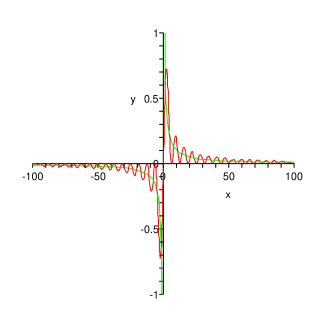
If all quantities that contain either of these functions are averaged or cannot be resolved over sufficiently long times, then we can set
| (116) |
[: principal value] thereby introducing little error.
If we re-insert the formal solution to Eq. (111) into Eqs. (109) and (110), we obtain the equations of motion of the atomic flip operators in the Markov approximation as
| (117) | |||||
| (118) |
where denotes the freely evolving electric field operator which, for example, describes the action of an external (classical) driving field. The symbols and are abbreviations for the following objects:
| (119) | |||||
| (120) |
whose relevance will become clear in the next section.
2.2.2 Spontaneous decay and Lamb shift
The equation of motion for the population inversion operator , Eq. (118), can be solved easily if no external electric field is present. In this case the equation of motion reduces to
| (121) |
Rewriting the inversion operator in terms of the projectors onto the excited and ground states, , we find for the excited-state projector the simple relation
| (122) |
Hence, the quantity determines the rate with which a two-level atom decays spontaneously from its excited state to its ground state.
Using the expansion (38), the decay rate Eq. (119) can be written as
| (123) |
which has to be understood in such a way that the function is placed under the mode sum. Hence, the rate with which the atom loses its excitation depends on the strength of the vacuum fluctuations of the electric field at the frequency of the atomic transition. In a certain sense, spontaneous decay can be viewed as stimulated emission driven by the fluctuating electromagnetic field. Using the plane-wave expansion (34), we obtain the well-known result for the spontaneous decay rate in vacuum
| (124) |
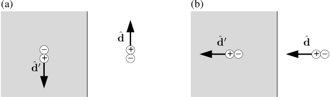
From the above, it should have become clear that the rate of spontaneous decay can be modified by altering the mode structure of the electromagnetic field. We have seen previously in Sec. 2.1.4 that the presence of boundary conditions for the electromagnetic field modifies the mode structure and hence the strength of the vacuum field fluctuations at the atomic transition frequency . As a simple example, let us consider a radiating dipole located close to a perfectly conducting mirror. Depending on its orientation with respect to the mirror surface, its rate of spontaneous decay is either completely suppressed or doubled with respect to its free space rate (Fig. 7). Suppression occurs when the dipole is parallel to the mirror and hence the dipole and its image are antiparallel and cancel each other [Fig. 7(a)]; doubling follows for perpendicular orientation where the dipole and its image are parallel [Fig. 7(b)].
The quantity that arises in the context of weakly interacting systems in the Markov approximation, Eq. (120), induces a shift of the atomic transition frequency, the Lamb shift. Rewriting the Lamb shift using the plane-wave expansion (34), we find
| (125) |
which is clearly infinite. This is yet another artefact of quantum theory in free space which can be remedied by mass renormalisation (for details, see e.g. Ref. [23]). For our purposes it is sufficient to argue that the ‘bare’ atomic transition frequency is unobservable because the interaction with the electromagnetic vacuum field can never be switched off and hence the only observable quantity is the renormalised frequency . However, in the following section we will again show how the presence of boundary conditions and, in particular, dielectric matter can modify the Lamb shift by an additional finite (and thus measurable) amount.
At this point it is perhaps interesting to observe that spontaneous decay and the Lamb shift are intimately connected by a causality relation analogous to the Kramers–Kronig relations that we will encounter in the next section. In fact, it is easy to see that and , taken as functions of the atomic transition frequency , form a Hilbert transform pair. Rewriting the integral (115) as
| (126) |
one observes that this is nothing else than the Fourier transform of the Heaviside step function . This in turn can be interpreted at the causal transform of the function , and the functions and are its real and imaginary parts. Due to the definition of a causal transform, and by Titchmarsh’s theorem [24], and and therefore and are Hilbert transform pairs and mutually connected via Kramers–Kronig relations. Hence, knowledge of the spontaneous decay rate at all frequencies gives access to the Lamb shift and vice versa.
2.2.3 Optical Bloch equations
In this section we will return to Heisenberg’s equations of motion for the atomic quantities in Markov approximation, Eqs. (117) and (118), and solve them under the assumption of an external driving field prepared in a single-mode coherent state with frequency . Hence, we set
| (127) |
In a frame that co-rotates with the angular frequency , Heisenberg’s equations of motion reduce to
| (128) | |||||
| (129) |
where is the detuning and denotes the Rabi frequency.
The density operator of any two-level (or spin-) system can be written in terms of the Pauli operators as
| (130) |
where is a real vector with norm and is the vector of Pauli matrices. Converting Eqs. (128) and (129) into equations of motion for the Bloch vector one finds the matrix equation
| (131) |
For negligible spontaneous decay , the Bloch equations take on the form of the gyroscopic equations
| (132) |
with . Its solution is then given by
| (133) | |||||
| (134) | |||||
| (135) |
Hence, the time evolution of the Bloch vector on time scales is described by precession of the Bloch vector with frequency along the surface of a cone with opening angle .
In the long-time limit, , the solution of the optical Bloch equations reaches its steady-state value. In the stationary state, when , the solution to the full Bloch equations is
| (136) |
In the weak driving limit, , the induced atomic dipole moment takes the form
| (137) |
whose real and imaginary parts fulfil the Kramers–Kronig relations when integrated over the mode frequency . Recall that both the spontaneous decay rate and the Lamb shift (via the detuning ) are contained in (137). In this weak-coupling regime, the induced dipole is thus described by a linear susceptibility. Its imaginary part, being proportional to the spontaneous decay rate , describes a loss channel for the incident field. The concept of linear-response functions and their role in the quantisation of the electromagnetic field in the presence of magnetoelectric matter will be detailed in Sec. 3.
2.2.4 Jaynes–Cummings model
In a sense the opposite limit to the case described in Sec. 2.2.3 is obtained if one considers a situation in which the mode structure of the electromagnetic field has been altered in such a way that discrete field modes interact with the atomic system. We have previously seen in connection with the Casimir effect (Sec. 2.1.4) that this can be achieved in resonators of Fabry-Perot type where the allowed modes in a cavity of length have discrete wave numbers . The half distance between two neighboring modes, , is called the free spectral range.
If a two-level atom with transition frequency is almost resonant with one of the cavity modes, one can treat the coupled atom-field system approximately by a single-mode model described by the Jaynes–Cummings Hamiltonian [25, 26, 27]
| (138) |
The coupling constant , which we have given the dimension of a frequency, can be read off from Heisenberg’s equations of motion as . Because we have assumed near resonance between atomic transition and the relevant cavity field mode, we have employed the rotating-wave approximation and subsequently dropped counter-rotating terms in the Hamiltonian (138).
The assumption that effectively only a single field mode interacts with the two-level atom implies a sharply peaked, comb-like, density of field modes. This requires a discretisation of the modes inside the cavity that can only be achieved with (almost) perfectly reflecting cavity walls. In reality, the material making up the cavity mirrors shows some transmission, part of which is of course wanted in order to be able to probe the cavity field from the outside. In effect, each of the cavity mirrors can be treated as a beam splitter (Sec. 2.1.3). For one-dimensional light propagation the equivalent potential encountered by the vector potential is a double barrier (Fig. 8).

Analytical solutions for the transmission coefficient have been first obtained in Ref. [28]. However, the problem becomes simpler by assuming that the barriers are functions with strength [29]. Then the transmission coefficient near one of the cavity resonances can be written as
| (139) |
where the line width is inversely proportional to the barrier height . Associating the barrier height with the squared index of refraction of the mirror material, one finds that the better the reflective properties of the mirrors [recall that ] the narrower the resonances.
The Jaynes–Cummings model is one of the few exactly solvable models of interacting quantum systems. The Hamiltonian (138) is in fact block diagonal in the basis ,
| (140) |
Its eigenfrequencies are
| (141) |
where we have defined the Rabi splitting which depends on the detuning and the -photon Rabi frequency .
The eigenstates of the Jaynes–Cummings Hamiltonian are superpositions of the unperturbed eigenstates ,
| (142) |
where the rotation angles are
| (143) |
For resonant interaction, , the unperturbed eigenstates are pairwise degenerate (Fig. 9). This degeneracy is lifted by the atom-field interaction. The level splitting depends on the number of photons. Note that even if there is initially no photon present, the exact eigenstates will be split by an amount , the vacuum Rabi splitting. This splitting, or ‘dressing’, of the bare energy levels is equivalent to the Lamb shift which we found in Sec. 2.2.2. However, it should be noted that the vacuum Lamb shift was due to the interaction with electromagnetic modes of all frequencies, whereas in the Jaynes–Cummings model the level shift arises from the interaction with a single discrete mode that has been selected by the resonator.
Because the Jaynes–Cummings Hamiltonian can be explicitly diagonalised, the unitary evolution operator is also known explicitly and reads
The last equality in Eq. (2.2.4) expresses the unitary time evolution in terms of the unperturbed eigenstates.
An important special case is the dispersive limit in which the detuning is large compared to the relevant -photon Rabi frequency, . In this limit, the level splitting can be approximated by , and the exact eigenstates are approximately the unperturbed eigenstates, and . Under this approximation, the unitary evolution operator can be written as
| (145) | |||||
or, with the free Hamiltonian ,
| (146) |
It is instructive to note that the evolution operator the dispersive limit, Eq. (146), is quadratic in the interaction strength . This means that it results in an effective nonlinear atom-field interaction. In order to investigate this claim in more detail, let us rewrite Eq. (146) in the following form. The term in square brackets contains, apart from a linear Stark shift of the excited state , a factor which is the result of an effective nonlinear Hamiltonian
| (147) |
Comparing Eq. (147) with the Jaynes–Cummings Hamiltonian (138) we see that the trilinear Hamiltonian (147) does not appear in the original Jaynes–Cummings model. The appearance of such an effective Hamiltonian is solely due the far off-resonant interaction. This is just one example of a generic nonlinear interaction such as those studied in Sec. 3.4.
3 Macroscopic quantum electrodynamics
Having established the framework of quantum electrodynamics in free space, we are now in a position to generalise the theory to magnetoelectric background materials. Before we go ahead with our program, let us first discuss the intrinsic difficulties associated with magnetoelectric media.
Let us assume we wanted to naively extend a plane-wave expansion of the electromagnetic field to include dielectrics. We would then try to replace the plane wave solutions to the Helmholtz equation by where is the index of refraction of the dielectric. In order to conform with standard requirements from statistical physics, the refractive index must be a complex function of frequency that satisfies the Kramers–Kronig relations
| (148) |
Due to the inevitable imaginary part of the refractive index, the plane waves are generically damped. That in turn means that they do not form a complete set of orthonormal functions needed to perform a Fourier decomposition of the electromagnetic field. The consequences of this failure are quite severe; either one insists on bosonic commutation rules for the photonic amplitude operators and which subsequently lead to wrong commutation relations between the operators of the electric field and the magnetic induction , or one postulates the correctness of the latter and ends up with amplitude operators in their Fourier decomposition that do not have the interpretation of annihilation and creation operators of photonic modes.
The reason for the failure of this naive quantisation scheme is easily found. The introduction of the index of refraction means that there exists an underlying (microscopic) theory that couples the free electromagnetic field to some dielectric matter, the effect of which is taken into account only by means of the response function . In doing so, the matter-field coupling is hidden from view but is nevertheless present. The damped plane waves have therefore to be regarded as eigensolutions of the combined field-matter system, and not of the electromagnetic field alone.
3.1 Field quantisation in linear absorbing magnetoelectrics
The above arguments necessarily lead one to consider the electromagnetic field interacting with an atomic system coupled to a reservoir that is responsible for absorption. An explicit matter-field coupling theory that achieves field quantisation in dielectric matter on the basis of a microscopic model has been developed by Huttner and Barnett [31, 30] (Sec. 3.1.1). This Hamiltonian model can be generalised to an effective Langevin noise model (Sec. 3.1.2) which forms the basis of the remainder of this article.
3.1.1 Huttner–Barnett model
Historically, the first successful attempt at quantising the electromagnetic field in an absorbing dielectric material is due to Huttner and Barnett [31, 30]. They considered a Hopfield model [32] of a homogeneous and isotropic bulk dielectric in which a harmonic oscillator field representing the medium polarisation is linearly coupled to a continuum of harmonic oscillators standing for the reservoir (first line in Fig. 10). Such a model leads to an essentially unidirectional energy flow — from the medium polarisation to the reservoir — which means that the energy is absorbed. Strictly speaking, because a single harmonic oscillator is coupled to a continuum, the revival time is infinite, hence an excitation stored in the continuum of harmonic oscillators will not return to the medium polarisation in any finite time. The overall system of radiation, matter polarisation, reservoir and their mutual couplings are regarded as a Hamiltonian system whose Lagrangian reads
| (149) |
where
| (150) | |||||
| (151) | |||||
| (152) |
Here and are the free Lagrangian densities of the radiation field and the matter, respectively, where and are the scalar and vector potentials in the Coulomb gauge (), and and the medium and reservoir oscillator fields with density , respectively. In the interaction part, , is the electric polarisability and the medium-reservoir coupling constants are assumed to be square integrable.
Upon introducing the canonical momenta
| (153) | |||||
| (154) | |||||
| (155) |
one can perform the Legendre transformation and construct a Hamiltonian . In Fourier space,
| (156) | |||||
| (157) |
are the longitudinal and transverse components of the vector potential and the matter polarisation, respectively. Similar decompositions are made for all other fields.
As in free space, one introduces mode amplitudes according to
| (158) | |||||
| (159) | |||||
| (160) |
where
| (161) |
The expressions (161) reflect the level shifts due to the interaction between fields. Indeed, we have encountered such shifts already in vacuum QED (Lamb shift, dressed energy levels in the Jaynes–Cummings model etc.). Similar decompositions can be made for the longitudinal fields which we will not consider here [33].
The amplitude operators are then promoted to Hilbert space operators with the usual bosonic commutation relations
| (162) | |||||
| (163) | |||||
| (164) |
The transverse Hamiltonian can be expressed in terms of the annihilation and creation operators as
| (165) |
with
| (166) | |||||
| (167) | |||||
| (168) |
where and . The Hamiltonian is clearly bilinear in all annihilation and creation operators, and can therefore be diagonalised by a Bogoliubov (squeezing) transformation, that is, by a linear transformation involving both annihilation and creation operators. In the present context, the procedure is known as a Fano-type diagonalisation [34].
The diagonalisation is performed in two steps. In the first step, the matter Hamiltonian is diagonalised first (second line in Fig. 10), leading to
| (169) |
In the second step, the dressed-matter operators and are combined with the photonic operators to the diagonal Hamiltonian
| (170) |
Diagonalisation of the longitudinal field components can be achieved analogously. Adding the resulting expression to Eq. (170) and Fourier transforming gives
| (171) |
which is depicted in the last line in Fig. 10. Due to the bosonic commutation relation of the amplitude operators, the commutation rule for the new dynamical variables are
| (172) |
Inverting the Bogoliubov transformation that has led to the polariton-like operators and and subsequent Fourier transformation leaves one with an expression for the vector potential and the polarisation field in terms of the dynamical variables and . The expansion coefficients turn out to be the dyadic Green tensor for a homogeneous and isotropic bulk material with a dielectric permittivity that is constructed from the microscopic coupling parameters , and [30, 35]. Later, this theory has been extended to inhomogeneous dielectrics where Laplace transformation techniques have been used to solve the resulting coupled differential equations [36]. However, neither of these expressions for the resulting fields contains any hints towards their underlying microscopic model, so it seems quite natural to start from the source-quantity representation of the electromagnetic field instead.
3.1.2 Langevin-noise approach
From now on, we leave the microscopic models behind and concentrate on the phenomenological Maxwell’s equations, assuming that the relevant response functions such as dielectric permittivity and magnetic permeability are known from measurements. Maxwell’s equations of classical electromagnetism, in the presence of magnetoelectric background media read, in the absence of other external sources or currents,
| (173) | |||||
| (174) | |||||
| (175) | |||||
| (176) |
They have to be supplemented by constitutive relations that connect the electric and magnetic field components. Assuming for a moment that the medium under consideration is not bianisotropic, we can write
| (177) |
where and denote the polarisation and magnetisation fields, respectively.
Polarisation and magnetisation are themselves complicated functions of the electric field and the magnetic induction . Assuming that the medium responds linearly and locally to externally applied fields, the most general relations between the fields that are consistent with causality and the linear fluctuation-dissipation theorem can be cast into the form
| (178) | |||
| (179) |
where and are the noise polarisation and magnetisation, respectively, that are associated with absorption in the medium with electric and magnetic susceptibilities and .
The Fourier transformed expressions (178) and (179) convert the constitutive relations (177) into
| (180) |
[] where
| (181) |
are the relative dielectric permittivity and (inverse) magnetic permability, respectively. An immediate consequence of the causal relation (181) is the validity of Kramers–Kronig (Hilbert transform) relations between the real and imaginary parts of the susceptibilities in Fourier space,
| (182) |
Using the expressions (181) for the dielectric permittivity and the magnetic permeability, Maxwell’s equations for the Fourier components can thus be written as
| (183) | |||||
| (184) | |||||
| (185) | |||||
| (186) |
Here we have introduced the noise charge density
| (187) |
and noise current density
| (188) |
respectively, which by construction obey the continuity equation.
Equations (185) and (186) now contain source terms. Hence, the electromagnetic field in absorbing media is driven by Langevin noise forces that are due to the presence of absorption itself. Moreover, the particular combination in which the noise polarisation and magnetisation enter Maxwell’s equations, Eq. (188), suggests that dielectric and magnetic properties cannot be uniquely distinguished. For example, one might include the magnetisation in the transverse polarisation in which case the constitutive relations (177) would have to be altered. This simple observation implies that the constitutive relations in the present form cannot be the fundamental relations. Instead, the noise current density appears as the fundamental source of the electromagnetic field. This becomes even more apparent if one allows for spatial dispersion that makes the dielectric response functions nonlocal in configuration space. It is therefore expedient to rewrite Eqs. (185) and (186) as
| (189) |
and to consider the most general linear response relation between the current density and the electric field in the form of a generalised Ohm’s law as
| (190) |
where is the complex conductivity tensor in the frequency domain [37].
The Onsager–Lorentz reciprocity theorem demands the conductivity tensor to be reciprocal, . The two spatial arguments must be kept separate in general, except for translationally invariant bulk media in which the conductivity only depends on the difference , i.e. in this case . We assume that, for chosen , the conductivity tensor is sufficiently well-behaved. By that we mean that it tends to zero sufficiently rapidly as and has no non-integrable singularities. However, functions and their derivatives must be permitted to allow for the spatially nondispersive limit. The real part of ,
| (191) |
is connected with the dissipation of electromagnetic energy and for absorbing media, as an integral kernel, associated with a positive definite operator [37]. Under suitable assumptions on the causality conditions satisfied by its temporal Fourier transform , the conductivity tensor is analytic in the upper complex half-plane, satisfies Kramers–Kronig (Hilbert transform) relations, and obeys the Schwarz reflection principle
| (192) |
We now identify the current density (190) as the one entering macroscopic Maxwell’s equations in the frequency domain. The medium-assisted electric field thus satisfies an integro-differential equation of the form
| (193) |
The unique solution to the Helmholtz equation (193) is
| (194) |
where is the classical Green tensor that satisfies Eq. (193) with a tensorial function source,
| (195) |
together with the boundary conditions at infinity. It inherits all properties such as analyticity in the upper complex half-plane, the validity of the Schwarz reflection principle, as well as Onsager–Lorentz reciprocity from the conductivity tensor, viz.
| (196) | |||||
| (197) |
In addition, the Green tensor satisfies an important integral relation that can be derived as follows. The integro-differential equation (195) can be rewritten as
| (198) |
where the integral kernel is reciprocal, from which Eq. (196) follows. With that, the complex conjugate of Eq. (198) reads
| (199) |
If we now multiply Eq. (198) from the left with and integrate over , then multiply Eq. (199) from the right with and integrate over , and finally subtract the resulting two equations, we find that for real the integral equation
| (200) |
Up until this point, all our investigations regarded classical electrodynamics. In order to quantise the theory, we have to regard the Langevin noise sources as operators with the commutation relation
| (201) |
which follows from the fluctuation-dissipation theorem associated with the linear response (190). In this way, the operator of the electric field strength is given by the operator-valued version of Eq. (194) as
| (202) |
The consistency of this quantisation procedure can be proven by checking the fundamental equal-time commutation relation between the operators of the electric field and the magnetic induction. Using Faraday’s law, Eq. (184), we find the frequency components of the magnetic induction field as
| (203) |
Hence, the equal-time commutator reads, on using the commutation relation (201) and the integral formula (200), as
| (204) |
where the second equality follows from the Schwarz reflection principle. Using the analyticity properties of the Green tensor in the upper complex half-plane, we then convert the integral along the real axis into a large semi-circle in the upper half-plane. From the integro-differential equation (195) and the properties of the conductivity tensor we find the asymptotic form of the Green tensor for large frequencies as
| (205) |
so that the equal-time field commutator takes its final form of
| (206) |
The striking feature is that the field commutator (206) is exactly the same as in free-space quantum electrodynamics [Eq. (40)], despite the presence of an absorbing dielectric background material. This fact reinforces the view that the fields and represent the degrees of freedom of the electromagnetic field alone and have little to do with any material degrees of freedom. The apparent discrepancy with the notion of the expansion (202) as a medium-assisted electric field is resolved by interpreting the Green tensor as the integral kernel of a projection operator onto the electromagnetic degrees of freedom. Finally, the Langevin noise currents can be renormalised to a bosonic vector field by taking the ‘square-root’ of the tensor (which exists because of its positivity in case of absorbing media). Writing
| (207) |
and defining
| (208) |
where
| (209) |
the expansion (202) of the frequency components of the operator of the electric field strength finally becomes
| (210) |
Hamiltonian:
In order to complete the quantisation scheme, we need to introduce a Hamiltonian as a function of the Langevin noise sources and or, equivalently, in terms of the bosonic dynamical variables and . Imposing the constraint that the Hamiltonian should generate a time evolution according to
| (211) |
the Hamiltonian must be of the form [38]
| (212) |
where is the inverse of the integral operator associated with . In terms of the bosonic dynamical variables, the Hamiltonian is diagonal,
| (213) |
which is its most commonly used form [39, 33, 40]. Perhaps surprisingly, it closely resembles its free-space counterpart, Eq. (37), in that it is bilinear in its dynamical variables. The reason behind this behaviour is that any linear reponse theory can be derived from an underlying microscopic model that is bilinear in its constituent amplitude operators which, after a suitable Bogoliubov-type transformation, leads to a Hamiltonian of the form (213). An example is provided by the Huttner–Barnett model of a homogeneous, isotropic dielectric (Sec. 3.1.1).
Spatially local, isotropic, inhomogeneous dielectric media:
We now apply the general theory to some special cases that are of practical importance. Let us begin with the simplest, and historically first, example of a spatially nondispersive, isotropic and inhomogeneous dielectric material that shows no magnetic response. The neglect of spatial dispersion makes the conductivity tensor strictly local, so that . Furthermore, isotropy means that . If we then make the identification where is the dielectric susceptibility, Eq. (210) becomes
| (214) |
which yields the well-known quantisation scheme for a locally responding dielectric material [39, 33, 41, 42, 43, 44, 45, 46].
Spatially dispersive homogeneous bulk media:
As a second example, we consider an infinitely extended homogeneous material for which is translationally invariant [38, 47]. That is, it is only a function of the difference . In this case, we represent as the spatial Fourier transform
| (215) |
A similar decomposition can be made for the integral kernel . For an isotropic medium without optical activity, the Fourier components can be written as [37]
| (216) |
and similarly for , where the expansion coefficients have to be replaced by their positive square-roots and
Clearly, the decomposition (216) is not unique as can be equivalently decomposed into
| (217) |
where
| (218) |
Since both and have to be real and positive to yield a positive definite integral kernel , the new variable is real, too. However, it does not have a definite sign. If, on the other hand, one forces to be positive, then the tensor
| (219) |
is the positive square-root of the integral kernel . The kernels and , despite being different, are related by a unitary transformation [38].
Spatially local magnetoelectric media:
The local limit of the above theory has a rather interesting structure. If one assumes that the functions and vary sufficiently slowly with and possess well-defined long-wavelength limits and , one finds the approximation
| (220) |
The full conductivity tensor associated with that real part (real and imaginary parts are related by a Hilbert transform) is then
| (221) |
with the identifications
| (222) |
where is the dielectric permittivity and the (para-)magnetic permeability of the medium. Note that the requirement implies that for , from which it follows that [4]. This in turn means that this theory can only describe paramagnetic materials. Diamagnetic materials are intrinsically nonlinear as their response functions themselves depend on the magnetic field and thus are excluded from a linear-response formalism.
The noise current density that is derived from the kernel
| (223) |
[which follows from Eq. (220)] can be decomposed into longitudinal and transverse parts according to with
| (224) | |||||
The distinction between longitudinal and transverse components of the noise current density (and subsequently the bosonic dynamical variables) is essentially a projection formalism, and the are termed projective variables [38].
Another, more frequently used decomposition is obtained by redistributing the electric part of the transverse noise current density. In this way, two new sets of independent bosonic variables, and , are introduced that lead to an equivalent decomposition of the noise current according to [40, 33]
| (226) | |||||
| (227) |
in which the possible spatial dependencies of the dielectric permittivity and the paramagnetic permeability have been reinstated (see Ref. [38] for details). The Hamiltonian (213) takes the form
| (228) |
Finally, the electric field (210) and the magnetic induction can be written as
| (229) | |||||
| (230) |
with the definitions
| (231) | |||||
| (232) |
where is the usual classical Green tensor satisfying Eq. (195). The latter Helmholtz equation condenses to (see also App. A)
| (233) |
For completeness, we mention that the integral relation (200) can be cast into the form
| (234) |
Statistical properties:
Thermal expectation values of the electromagnetic field can be obtained from those of the dynamical variables. Assuming the electromagnetic field in thermal equilibrium with temperature , it may be described by a (canonical) density operator
| (240) |
[: Boltzmann constant]. Thermal averages of the dynamical variables are thus given by
| (241) | |||||
| (242) | |||||
| (243) | |||||
| (244) |
where
| (245) |
is the average thermal photon number. This translates into the statistical properties of the electromagnetic fields as follows:
| (246) | |||||
| (247) | |||||
| (248) | |||||
| (249) | |||||
| (250) | |||||
| (251) | |||||
| (252) | |||||
These expressions will be needed for the calculation of relaxation rates (Sec. 4) and dispersion forces (Sec. 5).
3.1.3 Duality transformations
An important symmetry of the Maxwell’s equations in free space is duality where interchanging electric and magnetic fields yields the same differential equations. Here we will show that this type of symmetry can be established even within the framework of macroscopic quantum electrodynamics. At first, we consider macroscopic QED without external charges and currents. We group the fields into dual pairs and rewrite Maxwell’s equations as
| (254) |
where the constitutive relations are combined to
| (255) |
A general rotation in the space of dual pairs can be written as
| (256) |
It is easily checked that Maxwell’s equations (254) in free space with constitutive relations (255) is invariant under rotations of the form (256).
In the presence of spatially local magnetoelectric materials, the constitutive relations in frequency space can be further specified to
| (257) |
Invariance of the constitutive relations (257) under the duality transformation (256) requires that
| (258) |
which can be fulfilled in two ways. The first is obtained if the dielectric permittivity of the material equals its magnetic permeability, . This is achieved in free space as well as by certain metamaterials, for example by a perfect lens with [48]. In this case duality is a continuous symmetry which holds for all angles .
Generally, duality holds only for discrete values of the rotation angle, with . In this case, the transformation results in
| (259) |
It should be remarked that, not only are Maxwell’s equations invariant under the discrete duality transformation, but also the Hamiltonian that generates them.
| Partners | Transformation | ||
|---|---|---|---|
| , : | , | ||
| , : | , | ||
| , : | , | ||
| , : | , | ||
| , : | , | ||
| , : | , | ||
| , : | , | ||
| , : | , | ||
| , : | , | ||
To see this, one can derive the transformation properties of the dynamical variables from the relations (259) which read for as
| (260) |
These transformations obviously leave the Hamiltonian (228) invariant. Combining all relevant transformation relations, we can collect the duality relations for all electromagnetic fields, the linear response functions, and dipole moments, in Tab. 2. These relations allow one to establish novel results for magnetic (electric) materials and atoms in terms of already known results from their corresponding dual electric (magnetic) counterparts. Finally, duality does not only hold on the operator level in macroscopic QED without external charges and currents, but can also be established for derived atomic quantities. It is shown in Ref. [49] that dispersion forces as well as decay rates are all duality invariant, provided that the bodies are stationary and located in free space and that local-field corrections are applied when considering atoms embedded in a medium. The duality invariance of dispersion forces is further discussed and exploited in Sec. 5.
3.2 Light propagation through absorbing dielectric devices
In a previous section (Sec. 2.1.3) we developed the theory of quantum-state transformation at lossless beam splitters which accounts for a unitary transformation between the photonic amplitude operators associated with incoming and outgoing light. Unitarity is directly related to conservation of photon number during the beam splitter transformation. It is already intuitively clear that in the presence of losses, i.e. absorption, photon-number conservation and thus unitarity cannot be upheld, at least not on the level of the photonic amplitude operators. Having said that, because we have constructed a bilinear Hamiltonian of the electromagnetic field even in the presence of absorbing dielectrics, Eq. (228), there will be a unitary evolution associated with the medium-assisted electromagnetic field, but not with the (free) electromagnetic field alone.
In order to see how the restricted evolution emerges, we consider again a one-dimensional model of a beam splitter that consists of a (planarly) multilayered dielectric structure surrounded by free space (see Fig. 1). As opposed to a mode decomposition in the lossless case, we seek the Green function associated with the light scattering at the multilayered stack. In this one-dimensional model, the Green function reduces to a scalar function which can be constructed by fitting bulk Green functions at the interfaces between regions of piecewise constant permittivity [50]. Knowledge of the Green function amounts to knowledge of the transmission, reflection and absorption coefficients associated with impinging light of frequency . Similar decompositions can be made for three-dimensional structures with translational invariance [51].
It turns out that the input-output relations (56) have to be amended by a term associated with absorption in the beam splitter,
| (261) |
where denote (bosonic) variables associated with excitations in the dielectric material (device operators) with complex refractive index , and the absorption matrix. This expression is a direct consequence of the expansion of the electromagnetic field operators in terms of the dynamical variables. It is shown in Ref. [50] that the device operators are integrated dynamical variables over the beam splitter and read
| (262) |
where
| (263) |
The transmission and absorption matrices obey the relation
| (264) |
which serves as the generalisation of the above-mentioned energy conservation relation (52). Equation (264) says that the probabilities of a photon being transmitted, reflected or absorbed add up to one. Hence, photon numbers and thus energy is conserved only if one includes absorption. For a single plate of thickness surrounded by vacuum, the matrix elements read [50, 33]
| (265) | |||||
| (266) | |||||
| (267) | |||||
| (268) | |||||
The interface reflection and transmission coefficients are functions of the index of refraction and are defined as
| (269) |
and the factor accounts for multiple reflections inside the plate. These coefficients are special cases of the generalised Fresnel coefficients for -polarisation and normal incidence (see App. A.4).
The input-output relations (261) translate into a generalised quantum-state transformation formula. For this purpose, we need to look into an enlarged Hilbert space for the electromagnetic field and the dielectric object. With the four-dimensional vectors and , the input-output relations can be extended to a unitary matrix transformation of the form
| (270) |
where the unitary -matrix is an element of the group SU(4) and can be expressed in terms of the transmission and absorption matrices as [52]
| (271) |
where and . Given a density operator as a functional of the input operators , , the transformed density operator of the photonic degrees of freedom alone is then [52]
| (272) |
where denotes the trace over the device variables. As a first illustrative example, we consider the transformation of coherent states at an absorbing beam splitter. If we assume that both the incoming electromagnetic field as well as the beam splitter are prepared in two-mode coherent states and with respective amplitudes and , application of the input-output relations (261) [or equivalently, the quantum-state transformation (272)] reveals that the outgoing fields are prepared in a two-mode coherent state
| (273) |
Hence, the transformed amplitudes are determined not only by the transmission matrix but also by the absorption matrix [33].
This theory has wide-ranging applications that include nonclassicality studies of light propagation through optical elements and entanglement degradation in optical fibres [53, 54]. We mention here two important results relating to propagation of two-mode quantum states of light through optical fibres. Consider a two-mode squeezed vacuum state with squeezing parameter being sent through identical optical fibres of length that are held at a temperature . We regard the optical fibres as essentially one-dimensional objects whose effect on the quantum states of light propagating through them can be described by the input-output theory presented above. The optical fibres are characterised by their absorption length which implies that we approximate their transmission coefficient associated with them by . Furthermore, a nonzero temperature gives rise to a mean thermal photon number .
As a two-mode squeezed vacuum is a Gaussian state, it is fully characterised by its first and second moments, the mean and covariances of its Wigner function or characteristic function, respectively. For the quantum state under consideration, the mean is zero and its covariance matrix is
| (274) |
The covariance matrix transforms under an arbitrary completely positive map as
| (275) |
where is a positive symmetric matrix and an arbitrary matrix, provided that the resulting covariance matrix is a valid covariance matrix, i.e. obeys Heisenberg’s uncertainty relation [: symplectic matrix]. The non-orthogonality of the matrix is a direct consequence of dissipation, and is the additional noise as required by the fluctuation-dissipation theorem. The general structure (275) clearly also follows from the application of the quantum-state transformation formula (272).
Using the input-output relations (261), we find that the entries in the covariance matrix change according to [55]
| (276) |
which translates into a transformation of the covariance matrix as
| (277) |
from which the matrices and can be read off as and , respectively.
The entanglement content of a two-mode squeezed vacuum state, expressed in terms of its negativity [56], is . At zero temperature, and neglecting coupling losses into the fibres, the maximal amount of entanglement (in the limit of infinite initial squeezing) that can be transmitted through the fibres is . For finite initial squeezing, and at finite temperature , the state becomes separable, i.e. it loses all its entanglement, after the separability length
| (278) |
Note that at zero temperature this separability length is infinite, i.e. in this case it is always possible to transmit some entanglement over arbitrary distances.
3.3 Medium-assisted interaction of the quantised electromagnetic field with atoms
Up until now, our emphasis has been on devising a quantisation scheme for the electromagnetic field in the presence of magnetoelectric background materials, but without external sources. The starting point had been the definition of derived electromagnetic quantities such as the displacement field and the magnetic field in terms of the matter-related quantities and , the polarisation and magnetisation fields [Eq. (177)]. However, the definition of the latter is not unique as parts of them may be associated with magnetoelectric background media, whereas other parts could be attributed to additional atomic or molecular sources not included in the background matter. It is these additional sources that give rise to a successful theory of microscopic-dielectric interfaces.
In close analogy to the free-space case, the medium-assisted electromagnetic field can be coupled to an atomic system consisting of non-relativistic spinless charged particles via the minimal-coupling scheme. The dynamics of the combined atom-field system is governed by the Hamiltonian
| (279) | |||||
where
| (280) |
is the charge density of the particles. The vector and scalar potentials and of the medium-assisted electromagnetic field are expressed in terms of the dynamical variables and as
| (281) |
The total electromagnetic fields are the sums of the medium-assisted fields and the fields associated with the atomic system,
| (282) | |||||
| (283) | |||||
| (284) | |||||
| (285) |
where
| (286) |
is the scalar potential of the charged particles. In those cases in which the atomic system consists of sufficiently localised particles such as in an atom or molecule, it is expedient to introduce shifted particle coordinates relative to the centre of mass [with the total mass ]. Expanding the vector and scalar potentials and around the centre of mass, the Hamiltonian (279) simplifies for globally neutral atomic systems [] to the electric dipole Hamiltonian
| (287) |
where
| (288) | |||||
| (289) | |||||
| (290) |
Recall that the electric dipole moment is given by Eq. (102).
Equations (288)–(290) could form the starting point for investigations into interaction of the medium-assisted electromagnetic field with atomic systems in the long-wavelength approximation. However, as for free-space QED, the treatment can be considerably simplified by transforming using the alternative multipolar coupling scheme. To this end, we again apply a Power–Zienau transformation [20, 21, 22]
| (291) |
where the polarisation is still defined by Eq. (96), but the vector potential is given by Eq. (281) in the presence of magnetoelectrics, as opposed to the expansion (35) valid in free space. The unitary operator transformation with the operator (291) leads to transformed dynamical variables as [57]
| (292) |
and thus transformed electric fields (103). The magnetic induction field remains unchanged by this transformation, , because it clearly commutes with the operator of the vector potential. Other quantities that remain unchanged are those that depend solely on the atomic position operators such as the atomic scalar potential, , and the polarisation and magnetisation fields. The atomic momentum operators, however, transform as [57]
| (293) |
where we have defined the auxiliary vectors
| (294) | |||||
| (295) |
With these preparations, we can now write down the Hamiltonian (279) in terms of the transformed variables as
| (296) | |||||
It should be mentioned that, due to the unitary nature of the Power–Zienau transformation, the commutation relations between the transformed atomic position and momentum operators and as well as between the transformed dynamical variables and are unchanged. The fields and have to be thought of as being expanded in terms of the transformed dynamical variables in the same way as the untransformed fields are expanded in terms of the untransformed dynamical variables.
In the long-wavelength approximation, one replaces the function by its value at , , so that the polarisation and the auxiliary fields reduce to
| (297) |
Upon using these simplifications, we obtain the multipolar Hamiltonian (296) in long-wavelength approximation as
| (298) |
where
| (299) | |||||
| (300) | |||||
| (301) | |||||
where
| (302) |
is the magnetic dipole operator, , and .
At the moment, the magnetic dipole moment operator comprises only the contribution from the angular momentum. Spin can be included via a Pauli interaction term in Eq. (279) leading to
| (303) |
(: particle spin, : gyromagnetic ratio) [58].
The scheme can be easily extended to include more than one atomic subensemble. In the minimal-coupling scheme, this leads to interatomic Coulomb interactions in Eq. (279) which is why the multipolar-coupling scheme is strongly preferable. In this case, Eq. (298) generalises to [130]
| (304) |
where the dynamics of each atom is given by a Hamiltonian of the form (300) and each atom couples individually to the electromagnetic field via coupling Hamiltonians of the form (301).
As in the free-space case, we will henceforth treat all atom-field couplings within the framework of the multipolar coupling scheme and drop all primes denoting multipolar variables.
3.4 Nonlinear quantum electrodynamics
In all previous (as well as all subsequent) sections we have concentrated on magnetoelectric background materials whose dielectric (and magnetic) response to an external perturbation can be described within the framework of linear-response theory. That is, polarisation and magnetisation fields are linearly and causally related to the primary electromagnetic fields. For purely dielectric media, this means that [cf. Eq. (178)]
| (305) |
where is the dielectric susceptibility. However, many materials show nonlinear behaviour, i.e. their dielectric response has to be described by a polarisation with a component that depends quadratically (cubically, quartically etc.) on the external electric field. In free space where dispersion and absorption are disregarded and a mode expansions of the electromagnetic field can be used, the effect of these nonlinear polarisations is to add interaction Hamiltonians that are cubic (quartic, quintic etc.) in the photonic amplitude operators (see, e.g. [59]). These effective Hamiltonians arise from off-resonant interactions with atomic systems in rotating-wave approximation [see, e.g. Eq. (147)]. Our aim is to extend this theory to nonlinear processes in absorbing matter where mode expansions generally do not hold.
For this purpose, we consider an interaction Hamiltonian in its most general normal-ordered form corresponding to a medium. Using the abbreviation as a short-hand for the collection of spatial and frequency variables , this interaction Hamiltonian can be written as [60]
| (306) |
with an as yet unknown coupling tensor that will eventually have to be (linearly) related to the second-order nonlinear susceptibility . The integration initially ranges over all frequencies, even including those frequencies that would not guarantee energy conservation.
The Hamiltonian (306), together with the Hamiltonian of the linear theory (we include the index here to distinguish it from the nonlinear interaction Hamiltonian), is now used to construct the time-dependent Maxwell equations such as Faraday’s law as
| (307) |
The fields and have to be thought of as being expanded in terms of the dynamical variables and . Since Faraday’s law is valid irrespective of the presence of matter, and by definition , we must have
| (308) |
which is a condition that is needed in the next step. We write Ampère’s law , using Faraday’s law, as
| (309) |
where we split up the total displacement field into its linear part,
| (310) |
and some nonlinear polarisation . Heisenberg’s equations of motion then imply that
| (311) | |||||
where we kept only those terms that are at most linear in the coupling tensor . The terms that have been left out have to be included into higher order nonlinear processes. The first term on the rhs of Eq. (311) is by definition equal to the lhs of the same equation. The second term on its rhs vanishes because of the constraint (308). The remaining two terms have to satisfy
| (312) |
which yields a solution for the nonlinear polarisation . Note that the double commutator has been reduced to a single commutator as it turns out that a general solution would have to include functionals that commute with whose contributions can be shown to diverge [61] and thus have to be discarded.
The way to solve Eq. (312) is to view its rhs as being the Liouvillian generated by , i.e. , whose inverse can be formally written as
| (313) |
The action of the inverse Liouvillian on an operator is given by
| (314) |
which can be checked by direct calculation, with the result that
| (315) |
Before we continue solving this equation, we remark that due to the decomposition of the linear displacement field (310) into a reactive part and a Langevin noise contribution , the nonlinear polarisation also contains a contribution, , that disappears identically with vanishing absorption and can thus be regarded as the nonlinear noise polarisation. The result of the Liouvillian inversion can be cast into the form [60, 61]
| (316) | |||||
with
| (317) | |||||
and the notation .
From Eqs. (316) and (317) it is hard to see how the coupling tensor has to be related to the nonlinear susceptibility. Instead, we invoke comparison with the definition of the nonlinear polarisation from classical nonlinear response theory [59],
| (318) |
and introduce slowly varying electric fields whose (non-overlapping) amplitudes are centred at the mid-frequencies with such that
| (319) |
Expressing the electric fields in Eq. (319) in terms of slowly varying dynamical variables and comparing with the slowly varying version of Eq. (316) yields the sought after relation between and as [60, 61]
| (320) | |||||
where are the cartesian components of the Helmholtz operator, or equivalently, the integral operator associated with the inverse dyadic Green function.
Reinserted into the nonlinear interaction Hamiltonian (306), and combined with the dynamical variables, Eq. (320) will yield a formulation in terms of electromagnetic field operators. What becomes immediately clear, though, is that will not be of the form as in standard nonlinear optics. Mathematically, the reason is that there is no third Green tensor in Eq. (320). Instead, an inverse Green function (or Helmholtz operator) has to be dealt with which, by formally expanding it into a power series, will lead to additional contributions to the standard nonlinear interaction. The physical reason for this behaviour has to be sought in the fact that, from a microscopic point of view, an effective nonlinear interaction does not take place in free space but rather inside the absorbing medium where the local electric field is altered by the presence of the dielectric material. To account for that, local-field corrections such as those discussed in Sec. A.6 have to be included which automatically yields additional contributions to the nonlinear interaction Hamiltonian that are not of the standard form.
4 Atomic relaxation rates
The first set of applications we consider in this review regards the theory of atomic transition rates. In this section we discuss the influence of dielectric bodies towards atomic relaxation and heating rates, and some of their experimental ramifications.
To begin, it is necessary to study the dynamics of internal atomic degrees of freedom in the presence of absorbing magnetoelectric matter. In Sec. 3.3 we derived the Hamiltonian of the system comprising the medium-assisted electromagnetic field, the atomic system and their mutual interaction (here taken in the electric dipole approximation) as
| (321) |
with
| (322) |
the Hamiltonian of the medium-assisted electromagnetic field [Eq. (299)] in the presence of magnetoelectric bodies. The free atomic Hamiltonian [Eq. (300)] is expanded into atomic energy eigenstates ,
| (323) |
with the corresponding eigenenergies , and the atomic flip operators obeying the commutation rules
| (324) |
The electric-dipole interaction Hamiltonian which, in multipolar coupling, is given by [first term in Eq. (301)], is expanded in terms of the energy eigenstates as
| (325) |
where are the matrix elements of the dipole operator. Recall that we have dropped all primes on the electromagnetic field operators that indicate the multipolar coupling.
In similar fashion to the free-space theory outlined in Sec. 2.2.1, the internal atomic dynamics is governed by the solution to the coupled set of Heisenberg’s equations of motion ()
| (326) | |||||
and
| (327) |
We formally integrate Eq. (327) as
| (328) |
and reinsert this formal solution into Eq. (326) and obtain
| (329) | |||||
where
is the zero-point contribution to the internal atomic dynamics due to the second term in Eq. (328). A self-consistent solution is obtained if Eq. (329) is formally integrated as
| (331) | |||||
reinserted into Eq. (329), and (thermal) expectation values being taken. The are the shifted atomic transition frequencies. Using the thermal expectation values for the electromagnetic field operators given in Sec. 3.1.2, Eqs. (246)–(249), what remains is a set of coupled differential equations for the atomic quantities,
| (332) |
where the thermal contributions read ()
recall Eq. (4). These sets of equations form the basis for all following investigations in internal atomic dynamics.
4.1 Modified spontaneous decay and body-induced Lamb shift, local-field corrections
For weak atom-field coupling, these expressions can be further evaluated using the Markov approximation (see Sec. 2.2.1) in which the expectation values at times can be related to those at the upper limit of the time integrals as
| (334) |
The time integrals themselves are approximated as in the free-space theory by
| (335) |
Introducing the atomic density matrix elements , the set of differential equations reduces to
| (336) | |||||
| (337) |
These equations resemble closely those obtained in free-space theory. One can identify individual decay rates from state to , and total loss rates of a level . The individual rates contain zero-point [superscript ] as well as thermal [superscript ] contributions, , with
| (338) | |||||
Similarly, the shifted atomic transition frequencies depend on the frequency shifts where the zero-point and thermal contributions to the level shift induced by a single level read
| (340) | |||||
| (341) |
In , we have explicitly used the scattering part of the dyadic Green function because we assume that the vacuum-induced Lamb shift has already been included into the bare atomic transition frequencies .
Spontaneous decay of a two-level atom:
As an instructive example, let us consider a two-level atom with energy levels and separated by an energy which we assume to contain the free-space Lamb shift. At zero temperature, the spontaneous decay rate of the excited state is then given by Eq. (338) as [62, 63]
| (342) |
where we have neglected the shift in the atomic transition frequency . This is the same result one would obtain using perturbation theory, i.e. Fermi’s Golden Rule. We have noted previously that the rate of spontaneous decay in free space is proportional to the strength of the vacuum fluctuations of the electric field [Eq. (123)] which, by Eq. (249), is now seen to be proportional to the imaginary part of the dyadic Green function,
| (343) |
which underpins our interpretation of as the local density of states. The rate of spontaneous decay in vacuum, Eq. (124), is recovered by inserting the free-space Green tensor into Eq. (342).
To give a nontrivial example of how Eq. (342) can be used for investigating atom-surface interactions, we consider a two-level atom placed near a planar dielectric half-space with permittivity . The Green function for this structure is known (see Appendix A), and the result in the limit reads [64, 65]
| (344) |
Hence, a dipole oriented perpendicular to a planar surface decays twice as fast as a dipole parallel to it. Note the difference to the spontaneous decay rate near a perfect mirror which approaches finite values ( for perpendicular dipole orientation, for parallel dipole orientation) in the on-surface limit. In reality, however, nonradiative decay processes cause the near-field spontaneous decay rate to diverge.
Another important example, which has been used to investigate modified spontaneous decay inside a dielectric host medium [63, 33], is that of an atom in a spherical microcavity of radius (Fig. 11).

We use the dyadic Green function presented in Appendix A and note that, if the atom is located at the centre of the microcavity, only the TM-wave spherical vector wave functions do not vanish. Inserting the result into Eq. (342) yields [63, 33]
| (345) |
where the reflection coefficient for takes the form
| (346) |
[ and ]. In the near-field limit, i.e. when the size of the microcavity is much smaller than the atomic transition wavelength, we can expand in powers of and obtain [see also Eq. (633)]
| (347) |
[, ].
The leading terms in both examples, Eqs. (344) and (347), are proportional to the inverse cube of the atom-surface distance. This is attributed to resonant energy transfer to the absorbing dielectric surroundings which is a nonradiative decay process [66, 65, 67, 68, 69]. The next-to-leading terms, the induction terms, are proportional to the inverse atom-surface distance and correspond to absorption of real photons. The nonradiative decay rates make it impossible to hold atoms or molecules near dielectric or metallic surfaces and use their internal states for coherent manipulation. The correct quantum-statistical description of the dielectric bodies also imply that the suppression of spontaneous decay of a dipole parallel to a mirror surface (see Sec. 2.2.2) cannot be observed.
As the near-field contributions are proportional to the imaginary part of the permittivity, , these terms will vanish if absorption can be disregarded at the atomic transition frequency . In this case, the spontaneous decay rate is modified to [70, 63]
| (348) |
The results for a small spherical cavity can also be used to study the decay of atoms embedded inside a medium. In this real-cavity model, the cavity implements the local-field correction arising due to the difference between the macroscopic field and the local field experienced by the atom. Using the local-field corrected Green tensor from Appendix A.6 one can show that, for weakly absorbing media, Eq. (348) remains valid for arbitrary geometries when written in the form
| (349) |
where is the uncorrected decay rate. For absorbing media, the more general result
| (350) |
4.2 Sum rules for the local density of states
One of the principal cornerstones of macroscopic QED is the validity of Kramers–Kronig relations (182) for the response functions such as the dielectric permittivity, the magnetic permeability or the generalised conductivity. Equally important are sum rules that follow from asymptotic limits of these Hilbert transforms. Examples for sum rules in optics are the optical theorem that relates the imaginary part of the forward scattering amplitude to the total scattering cross section [2], or the Thomas–Reiche–Kuhn oscillator strength rule [72]. A particularly relevant relation for our purposes is the integral relation [73]
| (351) |
satisfied by the real part of the complex index of refraction . This follows from the superconvergence theorem for Hilbert transform pairs [74]. It means that the propagation properties of light in a dielectric medium are redistributed in such a way that, averaged over the whole frequency axis, the (real part of the) refractive index is the same as in vacuum.
Because macroscopic QED is inherently based on linear response theories, it is conceivable that quantities such as spontaneous decay rates would obey certain sum rules, too. Recall from Sec. 2.2.2 that the rate of spontaneous decay and the Lamb shift form a Hilbert transform pair. We will now try to derive a sum rule for the rate of spontaneous decay, and investigate integrals of the form
| (352) |
where is the free-space decay rate (124) and the scattering part of the dyadic Green function. Hence, we are seeking to compute the integral
| (353) |
where we have used the Schwarz reflection principle (197).
For the sake of definiteness, we imagine the radiating atom being placed inside a dielectric structure such as the spherical microcavity sketched in Fig. 11. In fact, any generic situation will involve an atom in free space surrounded by some dielectric material, although not necessarily in a spherically symmetric way. The scattering part of the dyadic Green function for any arrangement of dielectric bodies can always be expanded into a Born series (see Appendix A.5) as
| (354) | |||||
where is the free-space Green tensor and the dielectric susceptibility of the material surrounding the radiating atom. The integration extends over the total volume of the body, but excludes the location of the atom. The free-space Green tensor can be read off from Eqs. (538) and (539), setting . The first thing to note is that all terms containing the function involving the location of the atom do not contribute to the Born series.
As a function of , the free-space Green tensor has single and double poles at whose contributions to the integral (353) give rise to contributions that can be computed as follows. Concentrating on the first term in the Born series expansion, we need to look at contributions of the form with whose residues at are [75]
| (355) |
These terms arise from a short-distance or, equivalently, low-frequency expansion of the Green tensor. It is seen from Eq. (538) that they can be traced back to the longitudinal part of the free-space Green tensor. Hence, all these pole contributions, in any order of the Born series, arise from either purely longitudinal terms or from those in which one (and only one) of the longitudinal Green tensors has been replaced by a transverse part [75]. Subtracting these terms from the total scattering Green tensor,
| (356) | |||||
and noting that all other contributions containing non-negative powers of vanish after contour integration, it becomes obvious that
| (357) |
This in turn means that we can define a modified spontaneous decay rate which is constructed from , that obeys the sum rule
| (358) |
From its construction, it is clear that excludes dipole-dipole interactions. Because nonradiative contributions to the decay rate have been subtracted from , we can also interpret the sum rule (358) as a conservation of the integrated local density of states associated with photonic final states. Recalling our discussion following Eq. (351) this means that a magnetoelectric medium merely redistributes the photonic density of states across the frequency axis, but remain at the free-space level on average.
Finally, we make the connection to local-field corrections. The local-field corrected single-point Green tensor, obtained after discarding the terms containing in Eq. (633), is one example of a modified Green tensor (356) that leads to a valid sum rule for spontaneous decay rates. In this way, a connection is established to the theory in Ref. [76] which is strictly valid only in nonabsorbing materials.
4.3 Heating of polar molecules
In a previous section we argued that at very small atom-body distances, nonradiative decay will dominate. Given that this would require the atom or molecule to be held at distances much smaller than the (optical) wavelength, this effect will hardly be seen in a controlled experiment. The situation is changed dramatically when the transition wavelength in question is very large, say longer than a centimetre. This is the case for polar molecules since the spacings between neighbouring rotational and vibrational levels are relatively large. Molecules whose projection of the total orbital angular momentum vanishes () are best described by Hund’s coupling case (b) [77]. In this scheme, the molecular eigenstates are characterised by the quantum numbers and of the total angular momentum and its projection on the space-fixed -axis, the total spin quantum number (), the rotational quantum number () and the vibrational quantum number . For deeply bound states, the rotational and vibrational eigenenergies are [77]
| (359) |
where and are the rotational and vibrational constants, typical values of which are listed in Tab. 3.
| Spec. | ) | |||||
|---|---|---|---|---|---|---|
| LiH | ||||||
| CaF | ||||||
| BaF | ||||||
| YbF | ||||||
| LiRb | ||||||
| NaRb | ||||||
| KRb | ||||||
| LiCs | ||||||
| NaCs | ||||||
| KCs | ||||||
| RbCs |
Even at room temperature, the first few rotationally and vibrationally excited states may be considerably populated due to heating out of the ground state, placing severe limits on the coherent manipulation of polar molecules in their ground states. According to Eqs. (4.1), the respective heating rate is given by
| (360) |
where frequency shifts [Eqs. (340) and (341)] can typically be neglected. For a molecule in free space, use of the Green tensor (540) leads to [78, 79]
| (361) |
In order to evaluate these rates, the relevant dipole matrix elements need to be determined. For rotational transitions, this can best be done using Hund’s case (a) basis , where , and denote the projections of , and onto the internuclear axis (). In this basis, one has [77]
| (362) | |||||
where is the molecular dipole moment at the equilibrium internuclear separation, and
| (363) |
Relating the two bases via
| (364) |
one finds
| (365) |
for the molecules under consideration. For (ro-)vibrational heating, the dipole matrix elements follow from [77]
| (366) | |||
| (367) |
(: derivative of the dipole moment at equilibrium bond length, : reduced mass) to be
| (368) |
Combining the above results, one can calculate life times of polar molecules in free space against rotational and vibrational heating out of the ground state at room temperature () which are listed in Tab. 3. Since the rotational transition frequencies lie typically well below the maximum of the thermal spectrum ( at ), rotational heating mostly affects light molecules like LiH whose transition frequency is largest. For this molecule, rotational heating severely limits the life time of the ground state to about 2 seconds. Vibrational heating, on the contrary, mostly affects the fluorides whose vibrational transition frequencies are very close to the peak of the thermal spectrum; associated lifetimes lie in the range of a few seconds only. The rotational and vibrational heating rates exhibit strong temperature-dependences via the thermal photon number, so the impact of both heating channels can be considerably reduced by lowering the environment temperature.
Just like spontaneous decay, heating can be considerably enhanced when molecules are placed close to surfaces. Using the decomposition of the Green tensor into its free-space part and the scattering part accounting for the presence of the surface and recalling Eqs. (365) and (368), the ground state heating rate (361) can be written as [78]
| (369) |
(: atom-surface separation), where is given in App. A.4. Note that due to our neglect of the frequency shifts, Eqs. (340) and (341), the heating rate separates into the temperature-dependent factor as given by Eq. (361) and a purely position-dependent part.


In the nonretarded limit, , the position-dependence is approximately given by [78]
| (370) |
For metals with Drude permittivity
| (371) |
and for sufficiently small transition frequencies , one has
| (372) |
and the condition is not even valid for very small atom-surface separations. Instead, the heating rate is well approximated by the empirical formula [78]
| (373) |
which is valid for distances ( being the critical distance for which surface-induced heating becomes comparable to free-space heating).
In the opposite retarded limit, , the ground-state heating rate is approximately given by [78]
| (374) | |||||
where the second equality holds for good conductors. The distance-dependence is thus governed by attenuated oscillations away from the surface where the oscillation period equals twice the molecular transition wavelength.
The spatial dependence of the molecular heating rates over the entire distance rates is shown in Fig. 12 for CaF and NaCs. It is seen that vibrational heating dominates for CaF and results in rapid oscillations of the heating rate as a function of distance. For short distances, rotational heating strongly increases and begins to contribute to the total heating rate. For NaCs, rotational heating slightly dominates for moderate distances, although the oscillations associated with vibrational heating are still manifest in the total heating rate. At distance smaller than about , rotational heating becomes strongly dominant. The results show that molecular heating can strongly increase in close proximity to surfaces, thus placing severe limits on the miniaturisation of molecular traps.
4.4 Spin-flip rates
In cold-atom physics, where microengineered magnetoelectric or metallic structures are designed to magnetically trap ultracold atoms (e.g. 87Rb) in a well-defined Zeeman sublevel of their respective hyperfine ground states (cf. Fig. 13), typical transition frequencies range from (for reviews, see [80, 81, 82]).

The equivalent free-space wavelengths are thus on the order of several metres. As typical atom-surface distances are in the sub-millimetre range, the atoms are in the deep near field of the relevant (magnetic) transitions.
In complete analogy to electric-dipole transitions, we can investigate magnetic-dipole transitions using the approximate interaction Hamiltonian (301)
| (375) |
From the statistical properties of the electromagnetic field and our previously used arguments regarding Fermi’s Golden Rule we already know that the spin transition rate is proportional to the strength of the (thermal) magnetic field fluctuations, . If we assume an atom to be in its electronic ground state, the magnetic moment vector is proportional to the electronic spin operator (the nuclear spin operator is smaller by a factor of , i.e. the ratio between electron and proton mass; we also assume that the ground state has ). It can then be shown that the transition rate between two magnetic sublevels and is [84]
[, : Bohr magneton, ]. Note that this rate corresponds to the rates associated with electric transitions as given by Eqs. (338), (4.1) by means of a duality transformation , , cf. the transformation properties (528) and (529) of the Green tensor given in App. A.2. An experiment using 87Rb atoms in their hyperfine ground state has revealed spin flip lifetimes on the order of seconds for distances between [85]. Figure 14 shows the experimental data together with the theoretical predictions according to Eq. (4.4) where the Green function for a three-layered cylindrical medium was used [84] (see also App. A.4.2).


It is instructive to investigate certain asymptotic regimes in which analytical approximations to the expected spin flip lifetime can be given. For this purpose, we consider an atom at a distance away from a planar metallic surface with skin depth and with thickness . Its Green tensor can be found in App. A.4.1. The skin depth is related to the dielectric permittivity by . Together with the transition wavelength , there are four different length scales involved, of which is by far the longest and can be taken to be infinite. From the remaining three length scales one can find three experimentally relevant extreme cases that can be summarised in the following expression [86, 87]:
| (377) |
Here, is the trapping lifetime in free space which, for a transition frequency kHz, amounts to s [88]. For fixed values of () there are two distinct functional dependencies on the skin depth . These two scaling laws can be supported by rather intuitive explanations. If the skin depth is larger than the remaining length scales (i.e. the material is more dielectric), the magnetic field fluctuations weaken. As their strength is proportional to the imaginary part of the permittivity and hence the squared inverse skin depth, the lifetime increases quadratically with the skin depth [second and third lines of Eq. (377)]. If, on the other hand, the skin depth is the smallest length scale, the effective volume diminishes from which fluctuations emanate which leads to a lifetime increase with decreasing skin depth [first line in Eq. (377)].


This in turn means that there is a pronounced lifetime minimum when the skin depth is on the order of the atom-surface distance (Fig. 15). To either side of this minimum, the expected lifetime increases drastically. However, choosing a surface material with larger skin depth limits its capability to generate strong enough magnetic traps. On the other hand, natural materials with skin depths below at room temperature and are impossible to find.
A possible solution is to make use of superconductors on the assumption that due to the supercurrent magnetic field fluctuations are shielded away from the vacuum-superconductor interface, and hence spin transitions are suppressed. For a bulk superconductor with conductivity and , we can rewrite the first line of Eq. (377) as [89]
| (378) |
In the London two-fluid model [90] one assumes that the two types of charge carriers, normal and superconducting, react to an external field according to Ohm’s law and the London relation , respectively. As a function of temperature, the fraction of normal conducting electrons follows the Gorter–Casimir expression [91]. With the plasma frequency and the elastic scattering rate of the electrons, the conductivity can be written in the form
| (379) |
Although the two-fluid model does not fully capture the rich dynamics of superconductors (as it neglects coherence effects and dissipation), it gives a relatively accurate and intuitive picture of the strength of the magnetic field fluctuations. More elaborate models such as the Eliashberg theory prove that with regards to spin transitions the two-fluid model is perfectly adequate [89]. In Fig. 15 we show the distance-dependence of the spin flip lifetime for the two-fluid model of superconducting Nb (dashed line) and the corresponding results for an Eliashberg calculation with varying elastic scattering rates (symbols).
5 Dispersion forces
Dispersion forces such as Casimir forces between bodies [16, 92], Casimir–Polder (CP) forces between atoms and bodies [93, 94] and van der Waals (vdW) forces between atoms [94, 95] are effective electromagnetic forces that arise as immediate consequences of correlated quantum ground-state fluctuations. The total Lorentz force on an arbitrary macroscopic or atomic charge distribution characterised by a charge density and a current density occupying a volume is given by
| (380) |
To see how this quantum force acquires a nonzero average even in the absence of external electromagnetic fields due to correlated zero-point fluctuations, let us consider the example of a neutral, stationary ground-state atom . Expressing the atomic charge and current densities in terms of polarisation and magnetisation [recall Eqs. (96) and (97)], the Lorentz force can equivalently be represented as [57, 96, 97]
| (381) |
(: derivative with respect to the atomic centre-of-mass position). The quantum averages of both the electric and the magnetic field vanish in the absence of external fields, , and for an unpolarised and unmagnetised atom so do the atomic polarisation and magnetisation, . In the absence of correlations, this would imply that the average net force on the atom is vanishing, . However, both the electromagnetic and atomic fields are subject to nonvanishing zero-point fluctuations, , , , . These quantities are mutually correlated and thus lead to a nonvanishing dispersion force: For a nonmagnetic atom, one can show that this force is given by ([98], cf. also Sec. 5.2.1 below)
In accordance with the fluctuation-dissipation theorem, the real and imaginary parts of the atomic and field response functions (i.e. atomic polarisability and the Green tensor of the electromagnetic field) represent the reactive and fluctuating behaviours of these systems. Hence, the first term in the above equation correspond to the atomic zero-point fluctuations () giving rise to an induced electromagnetic field (), while the second term is due to the fluctuations of the electromagnetic field () giving rise to an induced atomic polarisation (). Both fluctuation sources thus contribute equally to the CP force. This interpretation is in contrast to the mode summation picture in which only the electromagnetic field fluctuations are taken into account, and the only role of the matter is to provide the perfect boundary conditions.
It is worth noting that for small separations, dispersion forces are primarily due to the atomic zero-point fluctuations which interact via the instantaneous Coulomb interaction. Dispersion forces where first postulated by J. D. van der Waals [99] and theoretically analysed by F. London [95] and J. E. Lennard-Jones [93] in this nonretarded limit. The zero-point fluctuations of the transverse electromagnetic field become important in the retarded limit of large separations, as was shown by H. B. G. Casimir and D. Polder [94]. To honour these two major steps, one often uses the notion vdW forces for all nonretarded dispersion forces on atoms and the term CP force for fully retarded ones — in contrast to the naming convention adopted throughout this work.
5.1 Casimir forces
The Casimir force (for general literature and reviews, see Refs. [100, 23, 101, 102, 103, 97, 104]) on a body of permittivity and permeability occupying a volume can be found by calculating the ground-state expectation value of the Lorentz force (380)
| (383) |
(: ground-state of the body-assisted electromagnetic field) where the coincidence limit must be performed in such a way that unphysical divergent self-force contributions are discarded after the vacuum expectation value has been evaluated. Using the relations
| (384) | |||||
| (385) | |||||
the field expansions (229), (230) and the expectation values (246)–(3.1.2), one finds for a homogeneous body at zero temperature [105]
| (386) |
where the coincidence limit has been performed by replacing the Green tensor with its scattering part. Here and in the following, the gradients and are understood to act on the first and second arguments of the Green tensor, respectively.
Alternatively, the Casimir force can be equivalently expressed in terms of a surface integral rather than a volume integral. To that end, one makes use of the relation
| (387) |
with the Maxwell stress tensor
| (388) |
This can be used to rewrite Eq. (383) in the form
| (389) |
[note that the last term in Eq. (387) does not contribute in the stationary case]. Evaluating the field expectation values according to Eqs. (246)–(3.1.2), one finds that () [106]
| (390) | |||||
The general expressions (5.1) and (390) can be used to calculate Casimir forces between bodies of arbitrary shape. In particular, Eq. (390) in connection with the Green tensor for planar multilayered dielectrics (App. A.4.1) immediately leads to the famous Lifshitz formula [92] for the Casimir force between two dielectric half-spaces [107]. In the limit of perfectly conducting plates, one recovers the mode summation formula (77).
5.2 Casimir–Polder forces
Similarly to the Casimir force, the Casimir–Polder force on a single atom (for a general overview, see Refs. [100, 108, 26, 109, 23]) can be calculated as an effective Lorentz force starting from expression (380), where the electromagnetic field acts on the atomic charge and current distributions. In general, this force is a time-dependent quantity which can only be found by solving the coupled atom-field dynamics [97, 96, 57]. In this section, we restrict our attention to the force on a ground-state atom with the body-assisted field being in its vacuum state, and we ignore the effect of motion on the CP force. For this stationary problem, the CP force can alternatively be derived from the atom-field coupling energy, following the approach originally used by Casimir and Polder [94].
Such an approach can be justified by means of a Born–Oppenheimer approximation by assuming that the fast internal (electronic) motion effectively decouples from the slow centre-of-mass motion. To see this, we express the total multipolar Hamiltonian (296) in terms of the centre-of-mass momentum and the internal momenta to obtain
| (391) |
where
| (392) |
[] is the internal atomic Hamiltonian associated with the electronic motion and the field Hamiltonian is given by Eq. (299). The influence of atomic motion on the atom-field interaction can be discarded by formally letting , leading to
| (393) | |||||
where the three terms describe the electric, paramagnetic and diamagnetic interactions with the electromagnetic field, respectively. Having thus separated the internal and centre-of-mass motion as far as possible, we can apply the Born–Oppenheimer approximation by integrating out the internal motion for given values of and , leading to an effective Hamiltonian for the centre-of-mass motion,
| (394) |
Here, is the energy of the uncoupled atom-field system and is the energy shift due to the atom-field coupling . Since we have neglected the influence of motion on the atom-field interaction, the energy shift does not depend on so that we may write
| (395) |
where is the well-known (free-space) Lamb shift (125) [23]. By means of the commutation relations , the effective Hamiltonian thus generates the following equations of motion for the centre-of-mass coordinate:
| (396) | |||
| (397) |
where the CP potential
| (398) |
is the position-dependent part of the energy shift, as suggested by Casimir and Polder. In many cases, the centre-of-mass motion is effectively classical and position and velocity in Eqs. (396) and (397) can be treated as -number parameters. In the following, it is not necessary to distinguish the classical from the quantum case and we drop the operator hats for convenience.
5.2.1 Perturbation theory
For weak atom-field coupling, the ground-state energy shift (395) can be obtained from a perturbative calculation. While the coupling Hamiltonian (393) presents very general basis for this purpose, the calculation can often be simplified by applying the long-wavelength approximation (which is valid provided that the atom-body separations are large with respect to the atomic radius) and neglecting the weak diamagnetic interaction, so that [cf. Eq. (301)]
| (399) |
This Hamiltonian being linear in both atomic and field variables, is to leading order given by the second-order energy shift
| (400) |
where denotes the (uncoupled) ground state of and the relevant intermediate states are those where the atom is excited, with a single-quantum excitation of the field being present, . The formal sum in Eq. (400) thus represents discrete summations over and the vector index as well as integrations over and .

Recalling the field expansions (229) and (230), the matrix elements of the electric and magnetic dipole interactions are found to be
| (401) | |||||
| (402) |
The matrix elements and the second-order energy shift are schematically depicted in Fig. 16. As the energy shift is quadratic in , it contains purely electric, purely magnetic and mixed electric–magnetic contributions. The latter are proportional to , so for nonchiral atoms, they can be excluded by means of a parity argument ( is odd and is even under parity). After substitution of Eqs. (401) and (402), we thus only retain the purely electric and magnetic terms, which upon using the integral relation (234) leads to
| (403) |
The Casimir–Polder potential (398) can be extracted from this energy shift by discarding the position-independent contribution associated with the bulk part of the Green tensor and only retaining its scattering part . The result can be further simplified by writing , making use of the Schwarz reflection principle, Eq. (197), and transforming the integrals along the real axis into ones along the purely imaginary axis (cf. Ref. [57]). The resulting ground-state CP potential is given by [100, 57, 96, 98, 110, 111, 112, 66, 113]
| (404) |
with
| (405) | |||||
| (406) | |||||
denoting the electric and magnetic parts of the potential and
| (407) | |||||
| (408) | |||||
being the atomic polarisability and magnetisability. The second lines of equalities in Eqs. (405)–(408) above hold for isotropic atoms.
When considering CP forces on atoms that are embedded in a body or a medium, one has to account for the fact that the local electromagnetic field interacting with the atom differs from the macroscopic one employed in our derivation. This difference gives rise to local–field corrections which can be implemented via the real-cavity model by assuming the atom to be surrounded by a small free-space cavity (recall the discussion in Sec. 4.1). In order to apply this procedure to our results (405) and (406), one has to replace the Green tensor by its local-field corrected counterpart as given in App. A.6 which, after discarding position-independent terms, results in [114, 58]
| (409) | |||||
| (410) |
where and denote the permittivity and permeability of the host body at the position of the atom. For an atom situated in free space, the local-field correction factors are equal to unity and one recovers Eqs. (405) and (406).
It is instructive to study the behaviour of the total CP potential under a duality transformation, which in this case amounts to a simultaneous global exchange and (see Tab. 2). Using the associated transformation laws (528) and (529) of the Green tensor as given in App. A.2, one sees that the duality transformation results in an exchange of the free-space potentials (405) and (406), so that the total potential is invariant with respect to a duality transformation [49]. The transformation laws (639) and (640) for the local-field corrected Green tensor imply that the same is true for an embedded atom, provided that local-field corrections are taken into account. The duality invariance of the CP potential is very useful when considering specific geometries: Once the electric CP potential of an atom in a particular magnetoelectric environment has been calculated, that of a magnetic one can be obtained by simply replacing and exchanging .
5.2.2 Atom in front of a plate
Let us apply the general results to an isotropic atom which is placed above () a magnetoelectric plate of thickness , permittivity and permeability , see Fig. 17.
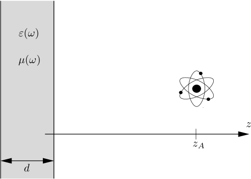
Using the Green tensor of this very simple geometry as given App. A.4.1, the electric CP potential (405) reads [96, 115]
| (411) |
where and are the reflection coefficients of the half space for - and -polarised waves and , with being the wave vector of these waves in free space. By virtue of the duality invariance, we can obtain the magnetic potential from the above expression by replacing and exchanging , which is equivalent to an exchange of and [cf. Eq. (555) in App. A.4.1] [116, 58]:
| (412) |
Perfect mirror:
A perfect mirror is realized for a perfectly conducting plate () or an infinitely permeable one (), in which cases the reflection coefficients are given by , respectively. In this particularly simple case, the -integrals in Eqs. (411) and (412) can be performed, so that the total CP potential (404) reads
| (413) |
where the upper (lower) is valid for the perfectly conducting (infinitely permeable) mirror. This result includes the famous Casimir–Polder potential of a polarisable atom in front of a perfectly conducting wall [94]. In the retarded limit (: minimum of all relevant atomic transition frequencies), the -integral is effectively limited to a region where the approximations and are valid and after integration one obtains [117]
| (414) |
In the non-retarded limit (: maximum of all relevant atomic transition frequencies), the factors and limits the -integral in Eq. (413) to a range where we may approximately set and neglect the second and third terms in the square brackets. The integral can then be performed with the aid of the definitions (407) and (408)
| (415) |
with the first term being the Lennard-Jones potential [93].
The results (413)–(415) show that a perfectly conducting plate attracts polarisable atoms and repels magnetisable ones. For the nonretarded limit, this behaviour can be made plausible by noting that the CP potential is due to the interaction of the atomic dipole moment with its image in the plate [93]. The image of an electric dipole moment , located at a distance away from a perfectly conducting plate, is constructed by a reflection at the -plane, together with an interchange of positive and negative charges and is hence given by , cf. Fig 18(a).
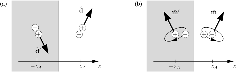
The average interaction energy of the dipole and its image is hence given by [118]
| (416) |
in agreement with Eq. (415), where the factor accounts for the fact that the second dipole is induced by the first one.
On the contrary, a magnetic dipole behaves like a pseudo-vector under reflection, so its image is given by , cf. Fig 18(b). The interaction energy of the magnetic dipole and its image reads
| (417) |
again in agreement with Eq. (415). The different signs of the CP potential associated with polarisable/magnetisable atoms can thus be understood from the different reflection behaviour of electric and magnetic dipoles.
Half space:
Let us next consider a semi-infinite magnetoelectric half space of finite permittivity and permeability, which is a good model for plates whose thickness is large with respect to the atom-surface separation. Using the reflection coefficients (555) in App. A.4.1, the electric and magnetic potentials (411) and (412) take the forms [96, 115, 119, 120, 116, 58]
| (418) | |||||
| (419) | |||||
with
| (420) |
where is the wave vector inside the half space. In the retarded limit (with being the minimum of all relevant atom and medium resonance frequencies) the potentials take the asymptotic forms [121]
| (421) | |||||
| (422) | |||||
[], while in the nonretarded limit (: maximum of all relevant atom and medium resonance frequencies), they are well approximated by
| (423) | |||||
| (424) |
for a dielectric half space and by
| (425) | |||||
| (426) |
for a purely magnetic one. One can summarise these results by stating that the CP potential is attractive for two objects of the same (electric/magnetic) nature, e.g. a polarisable atom interacting with a dielectric half space, while being repulsive for two objects of different nature.
In contrast to what is suggested by the findings for a perfect mirror, the different cases furthermore lead to different power laws in the nonretarded limit, with attractive potentials being proportional to and repulsive ones following a much weaker behaviour. When either the atom or the half space simultaneously exhibit electric and magnetic properties, both attractive and repulsive force components are present, which may be combined to form a potential barrier. This is illustrated in Fig. 19, where we show the potential (418) of a polarisable ground-state two-level atom near a magnetoelectric half space, whose permittivity and permeability have been modelled by the single-resonance forms
| (427) |
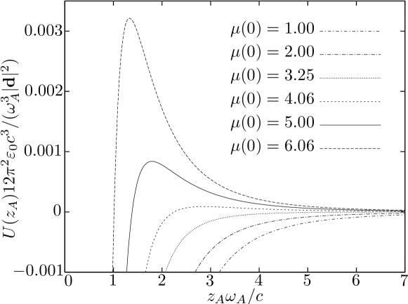
It is seen that repulsive force components may lead to a potential barrier at intermediate distances while attractive forces always dominate close to the surface due to their stronger power law. For a polarisable atom, repulsive force components are associated with the magnetic properties of the half space, so the barrier increases in height as increases. It follows from the retarded limit (421) that the threshold for barrier formation is for a weakly magnetoelectric half space and for a strongly magnetoelectric one.
Plate of finite thickness:
Finally, we consider a plate of arbitrary thickness . Use of the appropriate reflection coefficients (556) in Eqs. (411) and (412) leads to the potentials [115]
| (428) | |||||
| (429) | |||||

For a sufficiently thick plate, , one may approximate to recover the half-space results (418) and (419). In the opposite limit of a thin plate, , the approximation results in
| (430) | |||||
| (431) | |||||
As for the half space, these potentials reduce to simple power laws for large and small atom-surface separations. In the retarded limit, the thin-plate potentials read
| (432) | |||
| (433) |
while for nonretarded distances, they become
| (434) | |||||
| (435) |
for a purely electric plate and
| (436) | |||||
| (437) |
for a purely magnetic one. A comparison with the findings of Sec. 5.2.2 shows that when moving from a thick to a thin plate, all power laws are increased by one inverse power as a result of the linear dependence on . This similarity is due to the common microscopic origins of both forces (Sec. 5.4).
The general behaviour of the CP potential for a thin plate being very similar to that for thick plates, one may expect that repulsive force components may lead to potential barriers regardless of the plate thickness. This is confirmed in Fig. 20, where we display the potential (428) of a polarisable atom near plates of various thicknesses. We have chosen sufficiently strong magnetic properties to ensure the existence of a potential barrier. It is very low for a thin plate, reaches a maximal height for some intermediate thickness and then lowers slowly towards the asymptotic half space value as the thickness is further increased.
5.2.3 Atom in front of a sphere
As a second application of the general theory, let us consider an atom placed above at distance from the centre of a magneto-electric sphere of radius , permittivity and permeability , see Fig. 21.
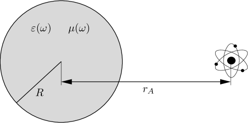
After substitution of the Green tensor (613) from App. A.4.3, the electric potential (405) in the presence of the sphere is given by [122]
| (439) |
where the sphere’s reflection coefficients for - and -polarised spherical waves read
| (440) | |||||
| (441) |
[, , , , , : spherical Hankel functions of the first kind, : spherical Bessel functions]. Using the duality invariance discussed in Sec. 5.2.1, the respective magnetic potential (406) can be obtained by making the replacements and , which as in the case of the half space amounts to an exchange :
| (442) |
In the limit of a large sphere, , the main contribution to the sums in Eqs. (439) and (442) is due to terms with large and one recovers the half-space results (423)–(426), as expected. For a sufficiently small sphere, , the sums effectively reduce to terms with , and one finds
| (443) | |||||
| (444) |
with and , where we have introduced the small sphere’s polarisability [118]
| (445) |
as well as its magnetisability
| (446) |
It is worth noting that in the small-sphere limit the electric and magnetic properties of the sphere completely separate. Furthermore, as will be seen in Sec. 5.3.2 below, the potentials (443) and (444) of an atom interacting with a small sphere have exactly the same form as that of two atoms, with the sphere’s polarisability and magnetisability replacing those of the second atom. In the retarded limit , the sphere potentials further reduce to
| (447) | |||||
| (448) |
while in the retarded limit one has
The hierarchy of signs and power laws of these potentials is closely analogous to that found for a half space or a thin plate: A polarisable atom is attracted to an electric sphere and repelled from a magnetic one, while the findings for a magnetisable atom are exactly opposite. Again, attractive and repulsive potentials follow the same () power laws in the retarded limit, while for short distances attractive potentials (with their power law) dominate over the repulsive () ones.
5.3 Van der Waals forces
The simultaneous interaction of two atoms with the electromagnetic field leads to the vdW force between them (for general literature and reviews, see [22, 97, 100, 123, 124, 125, 126, 127]), which may sensitively depend on their magneto-electric environment. In close analogy to the single-atom case, velocity-independent vdW forces between ground-state atoms can be derived from an atom-field coupling energy. Starting point is the two-atom generalisation
| (451) |
of the Hamiltonian (391), where the internal dynamics of the atoms is given by Hamiltonians of the type (392) and each atom individually interacts with the electromagnetic field via an interaction Hamiltonian of the form (393). Applying the Born–Oppenheimer approximation by integrating the internal atomic dynamics for given centre-of-mass positions , and momenta , , one obtains the effective Hamiltonian
| (452) |
Here, denotes the energy of the two uncoupled atoms and the field, and the energy shift
| (453) |
can be separated into a position-independent part (which contains the Lamb shifts of both atoms), two parts depending only on the positions of one of the atoms and a genuine two-atom part. The Hamiltonian (452) generates the following equations of motion for atom :
| (454) | |||
| (455) |
(similarly for atom ). The atom is thus subject to two forces, the CP force, which as discussed in the previous Sec. 5.2 can be derived from the CP potential (398), and the vdW force which is due to the additional atom. The associated vdW potential is given by the two-atom part of the energy shift
| (456) |
and it describes not only the direct, free-space interaction of the two atoms but also accounts for modifications of this interactions due to the presence of magnetoelectrics. As a consequence, Newton’s third law does not necessarily hold for the vdW force , due to the contribution of the bodies to the momentum balance.
5.3.1 Perturbation theory
In close analogy to the single-atom case, the vdW potential can for sufficiently weak atom-field coupling be obtained from a perturbative calculation of the energy shift. With each atom being linearly coupled to the electromagnetic field via an interaction (399), two-atom contributions start to appear in the fourth-order energy shift
| (457) |
where is now the (uncoupled) ground state of . In order to give a nonvanishing contribution to the energy shift, the intermediate states and must be such that one of the atoms and a single quantum of the fundamental fields are excited, while three possibilities exist for the intermediate states : Either both atoms are in the ground state and two field quanta are excited [], or both atoms are excited and the field is in its ground state or both atoms and two field quanta are excited. When invoking the additional requirement that each atom must undergo exactly two transitions, there is a total of ten possible combinations of intermediate states, which are listed in Tab. 4.
| Case | |||
|---|---|---|---|
| () | |||
| () | |||
| () | |||
| () | |||
| () | |||
| () | |||
| () | |||
| () | |||
| () | |||
| () |
The fourth-order energy shift (457) thus involves both transitions from zero- to single-quantum excitations and those between single- and two-quantum excitations of the electromagnetic field. The former are given by Eqs. (401) and (402), the latter can, upon recalling the field expansions (229) and (230), be found to be
| (458) |
| (459) |
with
| (460) |
Comparison with Eqs. (401) and (402) reveals that the matrix element for the one- to two-photon transition is equivalent to the two possible combinations of one photon being created and one propagating freely. This is schematically depicted in Fig. 22(a).
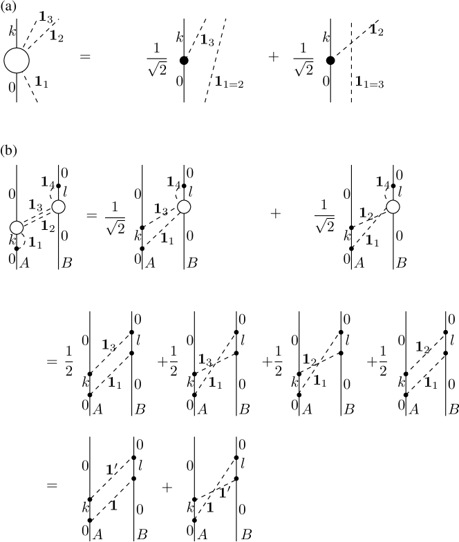
The various contributions to the vdW potential can be calculated by substituting the intermediate states from Tab. 4 and the matrix elements (401), (402), (5.3.1) and (5.3.1) into Eq. (457). Let us begin with the intermediate-state combination (1) from Tab. 4, the calculation of which is schematically represented in Fig. 22(b). After expanding the product in Eq. (457), evaluating the delta functions (460) and making use of the integral relation (234), one obtains
| (461) |
Note that the single- to two-photon transition (5.3.1) [or (5.3.1)] with its two possible processes [Fig. 22(a)] enters the energy shift quadratically, so after expanding the product, four different terms arise, see Fig. 22(b). They can be grouped into pairs of equal terms, so one ends up with only two distinct contributions. After assuming real dipole matrix elements, these two only differ in their frequency denominators and which are given in Tab. 5.
| Case | Sign | Denominator |
|---|---|---|
| () | , | |
| () | ||
| () | ||
| () | ||
| () | ||
| () | , | |
| () | ||
| () | ||
| () | ||
| () |
The energy shift (5.3.1) contains electric-electric contributions (where both atoms undergo purely electric transitions), magnetic-magnetic contributions (where both atoms undergo magnetic transitions) and mixed electric-magnetic and magnetic-electric ones. As in the single-atom case, we have assumed nonchiral atoms and discarded all those contributions where at least one atom undergoes an electric and a magnetic transition.
The contributions to the energy shift which are associated with the remaining intermediate-state combinations listed in Tab. 4 can be calculated in a similar way; all contributions are depicted in Fig. 23 (cf. also Ref. [22]).

The contributions (4)–(6), (9) and (10) contain two-photon states, so they correspond to two distinct terms, similar to the contribution (1) studied above. However, for the contributions (4), (5), (9) and (10), one of those two terms separates into two single-atom processes [diagrams (4b), (5b), (9b) and (10b) of Fig. 23] and does hence not contribute to the vdW potential. For real dipole matrix elements, all genuine two-atom contributions only differ from Eq. (5.3.1) by the frequency denominators and possibly also by the sign of the terms in the third and fourth lines of the equation; signs and denominators are listed in Tab. 5. The total vdW potential can be obtained by summing all contributions with the aid of the identity
| (462) |
which holds because the remaining parts of the integrands in Eq. (5.3.1) are symmetric with respect to an interchange of and . The -integral can be performed with the help of
| (463) |
Transforming the -integral to run along the positive imaginary axis, one finds [100, 128, 129, 130, 58]
| (464) |
| (465) |
| (466) |
| (467) |
| (468) |
where the atomic polarisabilities and magnetisabilities are given by Eqs. (407) and (408) and the respective second lines of these equalities hold for isotropic atoms. In close similarity to the single-atom CP potential (404)–(406), the two-atom vdW potential can hence be expressed in terms of the atomic response functions and the Green tensor of the electromagnetic field, where the latter connects the positions of the two atoms.
In order to treat the interaction of atoms which are embedded in a magnetoelectric, we have to generalise the above results by taking into account local-field effects. In close analogy to the single-atom case, this can be achieved via the real-cavity model by substituting the respective local-field corrected Green tensors (634), (636)–(638) from App. A.6 into Eqs. (5.3.1)–(5.3.1) resulting in [114, 58]
| (469) |
| (470) |
| (471) |
| (472) |
where and (and similarly for atom ).
The behaviour of the vdW potential under a duality transformation , follows immediately from the respective transformation laws of the Green tensor derived in Apps. A.2 and A.6. Using Eqs. (528)–(531), one sees that the free-space potentials (5.3.1)–(5.3.1) transform into one another according to , , so that the total vdW potential (464) is duality invariant [49]. The same is true for embedded atoms when including local-field corrections, as Eqs. (641)–(644) show. The duality invariance can be exploited when applying the general potentials to specific geometries; e.g., after calculation of for a certain magnetoelectric body, can be obtained by replacing and exchanging .
5.3.2 Two atoms inside a bulk medium
Let us first consider the vdW potential of two isotropic atoms that are embedded in an infinite homogeneous bulk medium of permittivity and permeability (Fig. 24).

Using the bulk Green tensor (537), the local-field corrected potentials (5.3.1) and (5.3.1) take the forms [114, 58, 131, 132]
| (473) | ||||
| (474) |
[; , refractive index of the medium] with and . Making use of duality invariance, we can apply the replacements , to directly infer the remaining two potentials [114, 58, 131, 132]
| (475) | ||||
| (476) |
These results and their retarded and nonretarded limits given below generalise the well-known free-space potentials [117, 133, 134, 135, 136]; in particular, reduces to the famous Casimir–Polder potential of two polarisable ground state atoms in free space for [94]. In free space, the potential between two electric or two magnetic atoms is attractive and that between an electric and a magnetic one is repulsive, in agreement with the general heuristic rule that dispersion forces between objects of the same electric/magnetic nature are attractive and those between objects of opposite nature are repulsive.
An inspection of Eqs. (473)–(476) reveals that a bulk magneto-electric medium can influence the strengths of the various two-atom interactions, but cannot change their signs. In order to discuss the effect of the medium in more detail, it is useful to consider the limits of large and small interatomic separations. In the retarded limit , the potentials are well approximated by
| (477) | |||||
| (478) | |||||
| (479) | |||||
| (480) |
In this case, the influence of the medium on all four types of potentials is very similar: The coupling of each atom to the field is screened by a factor for polarisable atoms, and a factor for magnetisable atoms; in addition, the reduced speed of light in the medium leads to a further reduction of the potential by a factor . In the nonretarded limit , the medium-assisted potentials simplify to
| (481) | ||||
| (482) | ||||
| (483) | ||||
| (484) |
The potentials and are thus again reduced, where in the nonretarded limit, is only influenced by the electric properties of the medium and only by the magnetic ones. On the contrary, the mixed potentials and are enhanced by a factor of up to in the nonretarded limit.
5.3.3 Two atoms near a half space
A modification of the vdW interaction does not only occur for atoms embedded in a medium, but can also be induced by a magnetoelectric body placed near to atoms in free space. To see this, let us consider the body-assisted vdW interaction of two atoms placed above () a semi-infinite half space of permittivity and permeability , see Fig. 25.

For simplicity, we assume both atoms to be isotropic and nonmagnetic, so that as given by Eq. (5.3.1). Separating the Green tensor into its bulk (free-space) and and scattering parts according to , the potential reads [130]
| (485) |
The first term is the free-space potential which is due to a direct exchange of two photons between the two atoms according to one of the various processes depicted in Fig. 23. The second and third terms represent the body-induced modification of the potential; they are due to processes where one or both of the two exchanged photons are scattered of the surface of the half space before being absorbed. The free-space part of the potential is just a special case of the bulk-medium potential (473) calculated in Sec. 5.3.2, while the body-induced change can be found by employing the free-space Green tensor (540) from App. A.3 together with the scattering tensor of the half space from App. A.4.1. As the resulting expressions are rather involved due to the large number of geometric parameters, we only give analytical formulae for some simple special cases.
Perfect mirror:
We first consider a perfect mirror, with the reflection coefficients being given by for a perfectly conducting plate and by for an infinitely permeable one. In the retarded limit , the vdW potential in the special case can be given in closed form [130, 137, 138]
| (486) |
(, ) where the first term in square brackets is the free-space potential due to the direct exchange of two photons and the second and third terms represent the mirror-induced modification of the potential due to scattering of one or two photons of the mirror surface (where the different signs refer to the two cases of a conducting or permeable mirror). An infinitely permeable plate thus always leads to an enhancement of the retarded interaction of two polarisable atoms whereas two cases need to be distinguished for a perfectly conducting one: When the atoms are aligned parallel to the plate (), Eq. (486) shows that the potential is always reduced due to the presence of the plate, while for a perpendicular alignment (), the potential of reduced if (atom being closer to the plate than atom ).
In the nonretarded limit , the vdW potential in the presence of a perfect mirror is found to be [130, 137, 138]
| (487) |
(). For a parallel alignment of the two atoms, a perfectly conducting plate thus reduces the vdW potential of two polarisable atoms while a permeable plate leads to an enhancement. In particular in the on-surface limit , the reduction and enhancement factors with respect to the free-space potential are given by and . On the contrary, for a vertical alignment the potential is reduced by a conducting plate while for a permeable plate it is reduced if (atom being closer to the plate than atom ).
The enhancement and reduction of the nonretarded vdW interaction due to a perfect mirror can be understood from the interaction of the fluctuating atomic dipole moments and and their images and in the plate, with
| (488) |
being the corresponding interaction Hamiltonian. Here, denotes the direct interaction between dipole and dipole , while and denote the indirect interaction between each dipole and the image induced by the other one in the plate. The leading contribution to the two-atom energy shift is of second order in ,
| (489) |
The three terms in Eq. (487) can be identified as different contributions to this energy shift: The first term is due to contributions that are quadratic in the direct interaction and is always attractive due to the global minus sign in Eq. (489). The third term which is associated with quadratic contributions of indirect dipole-image interactions or is attractive for the same reason and thus always acts as an enhancement of the free-space potential. The second term in Eq. (487) is due to mixed direct-indirect interactions, its sign is negative for attractive dipole-image interactions (thus tending to enhance the free-space potential) and positive for repulsive dipole-image interactions (leading to a reduction). The overall effect of the perfect mirror thus depends on the attraction or repulsion of the dipole-image interaction and, in the case of repulsion, on the relative strength of the mixed contributions compared to the purely indirect one.
We begin our investigations with the case of two (polarisable) atoms placed aligned parallel to a perfectly conducting plane. The image-dipole construction [Fig. 26(a)] reveals that the indirect interactions and are repulsive, explaining why the second term in Eq. (487) acts to reduce the interaction.
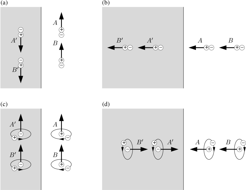
Equation (487) shows that it is always dominant over the enhancing purely indirect interaction, leading to an overall reduction of the free-space potential. The image-dipole construction further reveals that the quantity entering the mirror-induced modification of the potential is simply the distance between an atom and the image of the other atom. Let us consider next the case of perpendicular alignment of the two atoms. As seen from the image-dipole construction [Fig. 26(b)], the indirect interactions are attractive in this case, so that the mirror enhances the potential, in agreement with Eq. (487).

The case of two polarisable atoms near an infinitely permeable plate can be addressed by studying the interaction of two magnetisable atoms near a perfectly conducting plate instead, since the two problems are equivalent by virtue of duality. Noting that magnetic dipoles behave as pseudovectors under spatial reflection, one finds that for parallel alignment of the two atoms the dipole-image interaction is attractive [Fig. 26(c)] like the dipole-dipole interaction, so all mirror-induced terms enhance the free-space potential as predicted by Eq. (487). For perpendicular alignment the indirect dipole-image interaction is seen to be repulsive [Fig. 26(d)], so the mixed direct–indirect interaction tends to reduce the interaction [cf. the second term in Eq. (487)] while the purely indirect one acts towards an enhancement. For small atom-atom separations, the former clearly dominates due to the enhanced strength of the direct interaction, leading to a reduction of the overall potential while for large atom-atom separations, an enhancement due to the influence of the purely indirect interaction may be expected. The two cases are obviously separated by the inequality given below Eq. (487).
Magnetodielectric half space:
For a semi-infinite half space of finite permittivity and permeability , the vdW potential (5.3.3) is found by substitution of the free-space Green tensor (540) and the scattering Green tensor from App. A.4.1 together with the reflection coefficients (555) of the half space. The arising integrals over frequency and wave-vector components have to be solved numerically in order to obtain the half-space assisted potential for arbitrary interatomic and atom-half space distances. The results are shown in Figs. 27 and 28 for two identical two-level atoms with the permittivity and permeability of the half space being given by the single-resonance models (427), where we display the relative modification of the vdW potential with respect to its free-space value as found from Eq. (473).

Figure 27 shows the case of the two atoms being aligned parallel to the surface of the half space (). In agreement with the findings for a perfect mirror, Eqs. (486) and (487), the potential is always reduced by a purely dielectric half space [Fig. 27(a)] and enhanced by a purely magnetic one [Fig. 27(b)]. The relative reduction/enhancement becomes noticeable as soon as the interatomic separation becomes comparable to the atom-surface distance, it saturates for large interatomic separations. The figure further shows that the relative reduction for a dielectric half space has a pronounced minimum, the enhancement due to a magnetic one increases monotonically with interatomic distance.
In Fig. 28, we study the case of perpendicular alignment (). In agreement with the perfect-mirror results (486) and (487), a purely dielectric half space is found to always enhance the potential. The enhancement sets in when interatomic and atom-surface distances become equal, reaches a maximum in some cases (i.e., whenever the atom-surface separation of the closer atom is sufficiently small) and saturates for large interatomic distances. At first glance, the findings for a purely magnetic half-space seem to indicate a global enhancement which monotonically increases with the interatomic separation, thus being in contradiction with the perfect-mirror result (487). However, a closer look [cf. inset in Fig. 28(b)] reveals that for very small interatomic and atom-surface separations a reduction can indeed be found, as predicted by Eq. (487).
5.3.4 Two atoms near a sphere
In order to demonstrate the effect of different geometries on the vdW potential, consider next to polarisable atoms placed at distances and from the centre of a magneto-electric sphere of radius , permittivity and permeability , with the separation angle of the two atoms being denoted by , see Fig. 29.

The sphere-assisted vdW potential is given by Eq. (5.3.3) where the scattering Green tensor for the sphere can be found in App. A.4.3. For a small sphere () in the nonretarded limit (), one can show that the sphere-induced part of the potential reduces to [139]
| (490) |
[, , ] where is the polarisability of the sphere as given by Eq. (445). When replacing the sphere by a third atom (), our results coincides with the Axilrod–Teller potential of three atoms [140]. The sign of the three-body potential (490) depends on the geometric arrangement of the three objects. For instance, an attractive potential is found when they are placed in a straight line while the potential is repulsive when they form an equilateral triangle.
In Fig. 30, we show the total vdW potential of two identical two-level atoms placed at equal distance from a purely dielectric or purely magnetic sphere whose magnetoelectric response is given by Eqs. (427).

For small separation angles and atom-sphere separations, the sphere-induced modification of the vdW potential is very similar to our findings for two atoms placed in parallel alignment with respect to a half space: A dielectric sphere reduces the potential, while a magnetic one leads to an enhancement. However, the figure also shows that the behaviour is reversed as the angular separation grows. For an electric sphere, this enhancement of the potential for large angular separations can be understood from the fact that the Axilrod–Teller potential is attractive when the atoms and the sphere are situated on a straight line.
5.4 Relation between dispersion forces
The three types of dispersion forces considered in the previous three sections have a common origin and are thus closely related. To see this, let us start from the Casimir force (5.1) on a dielectric body of volume which is situated in free space and interacts with a second dielectric body of volume . Assuming the first body to consist of a dilute gas of atoms [number density , polarisability ] such that the linearised Clausius–Mosotti law [118]
| (491) |
holds, one can make use of the linear Born expansion given in App. A.5 to show that [105]
| (492) |
where is the Casimir–Polder potential (405). To leading order in the atomic polarisability, the Casimir force on the body is simply the sum of the CP forces on the atoms contained inside it. One can repeat the exercise for the second body to find
| (493) |
so the CP potential of each atom in body 1 with body 2 is due to its vdW interactions (5.3.1) with the atoms in body 2. Combining these results, one has [105]
| (494) |
Hence, to leading order the Casimir force between the two bodies is a sum over all possible vdW forces between atoms in body 1 and atoms in body 2. For weakly dielectric bodies, both Casimir and CP forces may thus be regarded as a consequence of two-atom vdW forces. These results naturally generalise to weakly magnetic bodies and magnetic atoms.
For bodies with a stronger magnetoelectric response, this simple additivity breaks down due to the influence of many-atom interactions [141, 142, 143, 144]. For instance, using the exact Clausius–Mosotti law [118]
| (495) |
together with the full Born expansion, one can show that the CP potential (493) generalises to [143, 144]
| (496) |
where denotes -atom vdW potentials [145, 146]. The full CP potential of a single atom in the presence of a body is just due to the whole hierarchy of its -atom interactions with the body atoms.
To illustrate the close relation between dispersion forces, let us look at a few simple examples, most of which have already been studied throughout this Sec. 5. In Tab. 6, we list signs and leading power laws of the dispersion forces between two atoms (Sec. 5.3.2), an atom interacting with a small sphere (Sec. 5.2.3), a thin ring [144], a thin plate (Sec. 5.2.2) and a semi-infinite half space (Sec. 5.2.2), and that between two half spaces [147, 148].
| Distance | Retarded | Nonretarded | ||
|---|---|---|---|---|
| Object combination | ||||
| Dual object combination | ||||
| (a) | ||||
| (b) | ||||
| (c) | ||||
| (d) | ||||
| (e) | ||||
| (f) | ||||
For weakly magnetoelectric objects, the rows (b)–(f) of the table follow by pairwise summation of the vdW forces displayed in row (a): Summation over the compact volumes of a small sphere (b) or a thin ring (c) does not change the respective power laws, while summation over an infinite volume lowers the leading inverse power according to the number of infinite dimensions. So, the leading inverse powers are lowered by two and three for the interaction of an atom with a thin plate of infinite lateral extension (d) and a half space (e), respectively. The power laws for the force between two half spaces (f) can then be obtained from the atom-half-space force (e) by integrating over the three infinite dimensions where integration over lowers the leading inverse powers by one while the trivial integrations over and yield an infinite force, i.e., a finite force per unit area. Note that all of these power laws remain valid for objects with stronger magnetoelectric bodies, so we can conclude that many-atom interactions do not change the asymptotic power laws.
The common features of all dispersion forces listed in the table are as follows: Forces between objects of the same (electric/magnetic) nature are attractive while those between objects of opposite nature are repulsive. The combinations and obviously lead to the same behaviour of the force as an immediate consequence of duality invariance, the same hold for the combinations and . Attractive and repulsive forces generally follow the same power law in the retarded limit, while in the nonretarded limit attractive forces are stronger by two inverse powers in the object separation.
5.5 Thermal effects
The Casimir–Polder force acting on a stationary atom at finite temperatures can be derived from the Lorentz force (381) which for a stationary nonmagnetic atom in electric dipole approximation takes the simple form
| (497) |
This expression can be evaluated using the statistical averages of the relevant electromagnetic field operators given in Eqs. (246)–(249). We use the multipolar-coupling Hamiltonian (298) in electric-dipole approximation to solve the coupled dynamics of the electromagnetic field and the atom which, upon using the solutions to the equations of motion for the internal atomic dynamics (Sec. 4), reads as [149]
| (498) |
After evaluating the integral in Markov approximation and the integral using countour-integral techniques, the thermal Casimir–Polder force on an atom in an incoherent superposition of energy eigenstates is given by with force components
| (499) |
[] and atomic polarisability
| (500) |
One important feature of the result (5.5) is the appearance of resonant force contributions proportional to and which are due to absorption and emission of photons, respectively. Even for ground-state atoms there exists a resonant force contribution
| (501) |
associated with absorption of thermal photons at the atomic transition frequency . This result is in contrast to the frequently used Lifshitz result [150]
| (502) |
which only contains the non-resonant force contributions. Clearly, because of the thermalisation of the atom, these resonant forces can only be observed on time scales that are short compared to the inverse ground-state heating rates . As their magnitude scales with the mean thermal number , the atomic transition frequency must not be too large in comparison with the ambient temperature, . Ideal candidates to observe these resonant force contributions would therefore be polar molecules whose vibrational and rotational frequencies are small enough to yield large thermal photon numbers at room temperature, and whose heating times can reach several seconds (see also Sec. 4.3) [78].
The atom thermalises after times much longer than and reaches its stationary (thermal) state
| (503) |
in the long-time limit. In this limit all resonant force contributions cancel, and the Casimir–Polder force can be written in the form (502) only if the atomic polarisability has been identified with the thermal polarisability
| (504) |
Without this identification, the equilibrium force (502) is generally larger than the one obtained from Eq. (5.5). The microscopic degrees of freedom of an atomic system thus give rise to a rich additional structure of CP forces, which is not explicitly present in the macroscopic Casimir force.
6 Cavity QED effects
In this final section, we turn our attention to the application of macroscopic QED to strong atom-field coupling scenarios. This is of particular interest in cases when the atom or molecule is confined in resonator-like structures in which the photon round-trip time is short compared to the atomic relaxation time.
6.1 Quantum-state extraction from a high- cavity
The interaction of a two-level atom with light in a resonant cavity is of fundamental importance to our understanding of quantum optics, and provides a playground to test ideas of quantum information processing such as the generation of entangled quantum states of two or more atoms [151] or the realization of single-photon sources. In a previous section (Sec. 2.2.4) we described the idealised situation of perfectly coherent atom-light interaction that led to the Jaynes–Cummings model. Within this model it is possible to completely transfer the excitation of a two-model atom to the cavity field and back coherently. The idea to use a high- cavity to deterministically generate single photons in well-defined quantum states is at the heart of cavity QED [152, 153]. Here we will examine the closely related problem of how to extract a photon from a cavity within the framework of macroscopic QED which provides us with the means to treat leaky cavities in a quantum-theoretically consistent way [51].
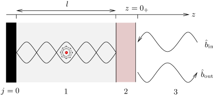
For simplicity, we will focus on one-dimensional cavities such as in Fig. 31 where region 0 denotes a perfect mirror, region 2 the semi-transparent mirror, region 1 the cavity interspace, and region 3 the free space surrounding the system. In order to calculate the response of the atom-cavity system, we assume that the atom is initially being prepared in its excited state and the cavity field is in its ground state . Then, the state vector at a later time can be expanded into
| (505) |
The Schrödinger equation with the electric-dipole Hamiltonian (301) yields coupled equations of motion for the unknown coefficients and as
| (507) |
[: cross-sectional area of the cavity]. Inserting the formal solution of Eq. (507) into Eq. (6.1) yields an integro-differential equation
| (508) |
with the integral kernel
| (509) |
The spectral response is carried by the Green function which has to be determined by adjusting the boundary conditions at the interfaces between the regions of piecewise constant permittivity. Because of multiple scattering inside the cavity region 1, the Green function has poles at the complex frequencies where the condition
| (510) |
[: generalised Fresnel reflection coefficient (556)] is met. We assume that the line widths are much smaller than the line separations so that the integration over frequency in the kernel can be restricted to subintervals . Near a cavity resonance, the time integral in Eq. (508) can then be performed in the Markov approximation to provide the cavity-induced shift of the atomic transition frequency as [51]
| (511) |
with
| (512) |
[]. Within these approximations, the kernel function for the excited-state probability amplitude is then
| (513) |
The solution for is the prerequisite for the calculation of the photon extraction efficiency from the cavity [51], which is defined as the probability of having the outgoing field prepared in a single-photon Fock state. The result for a typical situation is shown in Fig. 32.
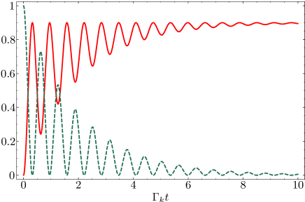
For very long times, a sufficiently high- cavity and almost exact resonance, the extraction efficiency approaches . Here, the is the radiative damping rate and the transmission coefficient . The decay rate of a cavity resonance is the sum of the radiative damping rate and the absorptive damping rate where is the absorption coefficient at the cavity resonance frequency . Hence, the extraction efficiency in the stationary limit is [154, 155]
| (514) |
For intermediate times, the efficiency shows an oscillating (tidal) behaviour. Thus, during each emission/re-absorption cycle within the cavity, the single-photon wave function builds up outside the cavity until the steady-state solution (empty cavity) is reached.
6.2 Spherical microcavities
Spherical microresonators possess a rich structure of field resonances to which an atom can be coupled when placed inside (whispering gallery modes) or outside (surface-guided modes) the resonator.
6.2.1 Atom inside a spherical microcavity
In cases in which the atom is embedded in a spherical microcavity, we can distinguish between large and small cavities, weak and strong coupling. In Sec. 4.1 we have discussed the case in which an atom was placed inside a very small cavity. This led us to the notion of local-field corrections. We now have a brief look at a cavity whose radius is much larger than the relevant atomic transition frequency. In view of the three-layered structure depicted in Fig. 33, we thus require that .
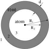
Then, the rate of spontaneous decay can be calculated from Eq. (346) in the limit of thick cavity walls as [156]
| (515) |
The left panel in Fig. 34 depicts the normalised decay rate as a function of frequency. We assume a single-resonance Drude–Lorentz model (427) with and . The microresonator has parameters and . One observes narrow-band enhancement () alternating with broadband suppression () of spontaneous decay. The narrow peaks are located at the cavity resonances.


When the atomic transition frequency approaches one of the cavity resonances, the atom-field coupling becomes stronger. At resonance, when where is one of the resonance frequencies of the microcavity, the time evolution for the excited-state occupation probability is the one of a damped oscillator with damping constant , the width of the cavity resonance. For small material absorption, , the cavity resonance line can be approximated by a Lorentzian with width
| (516) |
In the strong-coupling regime when the condition is fulfilled, the excited-state probability
| (517) |
shows damped Rabi oscillations with Rabi frequency . The right panel in Fig. 34 shows the temporal evolution of the excited-state occupation probability for , , and (solid line), (dashed line), and (dotted line). The other parameters are the same as those used for the curves in the left panel. For comparison, the exponential decay in free space is also shown (dashed-dotted line).
6.2.2 Atom outside a spherical microcavity
Atoms need not be located inside a closed dielectric or metallic structure in order to be coupled strongly to the electromagnetic field. Instead of whispering gallery modes that are due to total internal reflection inside a sphere, surface-guided modes can be excited on the outside surface of a spherical microcavity [157]. Assuming again a Drude–Lorentz model for the permittivity of the dielectric sphere that features a band gap between the transverse resonance frequency and the longitudinal resonance frequency . It is clear that for frequencies below () whispering gallery modes are excited, whereas for frequencies within the band gap () surface-guided modes are excited.
Figure 35 shows the rate of spontaneous decay of a radially oriented dipole very close () to a microsphere of radius .
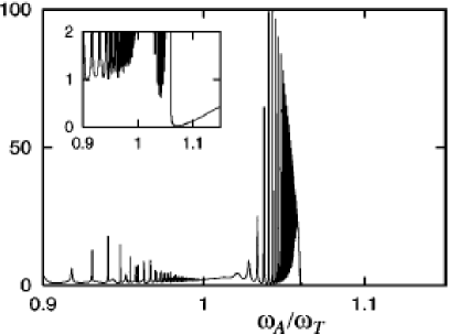

In this near-field limit, the decay rate is approximately given by Eq. (344) for a planar interface,
| (518) |
The strong enhancement in the band-gap region () is due to surface-guided modes.
These surface excitations can be used to induce entanglement between two atoms located diametrically opposite around the microsphere [157, 159]. If the two atoms and are initially prepared in their respective excited and ground states, their combined initial state can be written in terms of the (entangled) coherent superpositions which are initially equally excited. Associated with these superpositions are decay rates
| (519) | |||||
[; and , spherical Bessel and Hankel functions; , generalised reflection coefficient given in Sec. A.4.3]. If the atomic transition frequency coincides with one of the microsphere resonances , the single-atom decay rate can be approximated by [158]
| (520) |
and therefore the decay rates of the superposition states reduce to . This means that if is even (odd), the state () decays much faster than the state (). The frequency dependence of is shown on the right panel in Fig. 35. Hence, depending on one of the superposition states is superradiant while the other is subradiant. After the superradiant combination has decayed, the two atoms reside in the subradiant entangled state or .
7 Outlook
The theory of macroscopic quantum electrodynamics is a powerful tool that provides the link between isolated atomic ensembles and absorbing solid-state surfaces. It extends the well-established field of free-space quantum optics to new horizons. It is remarkable that, at least within the framework of causal linear response, one finds a Hamiltonian description of the medium-assisted electromagnetic field that does not have to fall back onto a master equation description. Instead, unitary evolution equations can be found that take into account absorption processes as well. Examples of such unitary evolutions include the absorbing beam splitter (Sec. 3.2) and internal atomic dynamics (Sec. 4). In many cases, macroscopic quantum electrodynamics can provide more information than perturbative calculations, as exemplified by the theory of thermal Casimir–Polder forces (Sec. 5.5).
Obvious extensions towards nonlinear interaction Hamiltonians (Sec. 3.4) will be further studied to bridge the gap between classical descriptions of nonlinear processes to include both linear and nonlinear absorption, and to establish the connection with microscopic models of effective nonlinear interactions. Such a theory is likely to provide detailed information on the quantum state of light that emerges from, e.g. spontaneous parametric down-conversion crystals, and on the effect of higher-order nonlinearities.
As it is evident from our collection of examples, for the time being we have always assumed that all macroscopic bodies as well as all atomic systems are at rest. Such a restriction is clearly not necessary. Centre-of-mass motion of atomic systems can be accounted for by either imposing a classical trajectory or more consistently by solving Newton’s equations of motion in addition to Maxwell’s equations. To assume a classical trajectory for an atom or a molecule means to neglect the backaction onto the motion which in many cases can be justified.
For example, from our discussion in Sec. 5 it is clear that an atom moving parallel to a planar dielectric surface will not only experience a Casimir–Polder force in the direction perpendicular to its motion, but also in the direction of its motion. This effect is sometimes called quantum friction and can be understood in two ways. In our intuitive picture of Casimir–Polder forces being caused by forces between the atomic dipole and image dipoles in the magnetoelectric material, one can view quantum friction as a drag effect acting on the image dipoles due to finite conductivity or even resonances. Another way to view quantum friction is as an interaction with the surface plasmon at the magnetoelectric interface.
Taking the quantum-mechanical character of atomic position and momentum into account will lead one to a theory of motional heating that is important in particular in ion traps. The opposite effect of cooling to the motional ground state, enhanced by coupling to a resonant microcavity, can also be understood within the framework of macroscopic quantum electrodynamics.
Eventually, understanding how motion affects dispersion forces acting on isolated atomic systems will lead to a theory of a quantum theory of moving dielectric materials which thus far only exists for strictly non-absorbing materials. This in of fundamental interest as it makes contact with the low-energy limit of effective action in quantum field theory.
This work was financially supported partially by the UK Engineering and Physical Sciences Research Council and the Alexander von Humboldt foundation. The authors are grateful to all our colleagues who contributed to the theory of macroscopic quantum electrodynamics, in particular D.-G. Welsch who was involved in developing this theory from the very beginning, J.A. Crosse, H.T. Dung, R. Fermani, M. Khanbekyan, L. Knöll, C. Raabe, H. Safari, A. Sambale, M.R. Tarbutt, A. Tip, and M.S. Tomaš. We thank E.A. Hinds and P.L. Knight at Imperial College London for their continuous support, and the staff at the Gloucester Arms for hospitality during our Doppelkopf sessions.
Appendix A Dyadic Green functions
The notorious problem one perpetually faces in macroscopic QED is to find the Green tensor or dyadic Green function (DGF) associated with the classical electromagnetic scattering problem. This is not unusual as the DGF generalizes the usual mode expansion in free space to the solution of a more general boundary value problem. In what follows we will restrict ourselves to the special case of spatially local magnetoelectric materials. Extensions to materials with spatial dispersion can be found in Ref. [38].
We will need to look for the fundamental solution to the Helmholtz equation
| (521) |
with the dielectric permittivity and inverse magnetic permeability being arbitrary. The solution to Eq. (521) can be written in terms of the DGF as
| (522) |
where the dyadic Green function satisfies
| (523) |
Together with the boundary condition that vanishes as , Eq. (523) has a unique solution provided that the strict inequalities and hold. Physically, these requirements mean that all dielectric materials have to be passive, i.e. absorbing, media.
A.1 General properties
The dyadic Green function inherits the analytical properties of the permittivity and permeability. That is, it is meromorphic in the upper complex frequency half-plane, and the Schwarz reflection principle
| (524) |
holds. The Onsager reciprocity theorem requires that the DGF satisfies the additional relation
| (525) |
Particularly useful is the following integral relation involving products of Green functions,
| (526) | |||||
This relation is essentially the linear fluctuation-dissipation theorem, written in terms of the dyadic Green function.
A.2 Duality relations
Another useful property of the DGF is its behaviour under a duality transformation. The dual DGF is defined by the equation
| (527) |
with , , i.e., it is the solution to the Helmholtz equation with and exchanged. By applying the duality transformation to the field expansions (236)–(239), using the transformation rules listed in Tab. 2 and comparing coefficients, one can easily verify the following relations between the original DGF and its dual [49]:
| (528) | |||||
| (529) | |||||
| (530) | |||||
| (531) |
In the next subsections, we will list the explicit forms of dyadic Green functions for important highly symmetric geometric arrangements of magnetoelectric bodies.
A.3 Bulk material
The simplest situation one can envisage is one of a homogeneous, isotropic dielectric medium. In this case, the dielectric permittivity and magnetic permeability do not depend on the spatial position. This means that the magnetoelectric material and hence the dyadic Green function that describes it must be translationally invariant. Thus, the DGF can only depend on the difference between the coordinates , . We can therefore use Fourier transform techniques to solve Eq. (523). Defining
| (532) |
the Fourier transformed Helmholtz equation is
| (533) |
This is now an algebraic equation that can be easily solved. To do so, we decompose the unit tensor into its transverse and longitudinal parts with respect to the wave vector ,
| (534) |
Note that
| (535) |
is transverse. Hence, the Green tensor is, after inserting into the inverse Fourier transform,
| (536) |
which can be transformed back into configuration space using contour integral methods. Noting that the dielectric permittivity and the magnetic permeability have no poles or zeros in the upper complex frequency half-plane, the result is
| (537) |
[]. After evaluating the derivatives one arrives at a decomposition into transverse and longitudinal parts as
| (538) | |||||
| (539) | |||||
In particular, in free space where , we find that
| (540) |
with and .
A.4 Layered media: planar, cylindrical, spherical
A more challenging situation arises if one considers magnetoelectric materials that are structured to form boundaries of certain symmetry. What we envisage here are examples of stratified materials in planar, cylindrical and spherical geometries. The idea is to expand the dyadic Green function in terms of vector wave functions associated with the symmetry of the problem. The success of this procedure is directly related to the problem of separability of the Helmholtz operator . There are only a few coordinate systems in which this operator is separable [160], namely the cartesian, cylindrical, spherical and spheroidal coordinate systems. Hence, only there can the solution to the three-dimensional Helmholtz operator be reduced to seeking the scalar solution of a one-dimensional wave equation.
The scalar Helmholtz equation takes the form
| (541) |
[]. Table 7 lists the scalar eigenfunctions that are regular at the origin for cartesian, cylindrical and spherical coordinate systems.
| coordinate system | pilot vector | scalar eigenfunctions |
|---|---|---|
| cartesian () | ||
| cylindrical () | ||
| spherical () |
The scalar wave function is then used to construct the irrotational () and solenoidal ( and ) eigenfunctions with respect to a pilot vector as [161]
| (542) | |||||
| (543) | |||||
| (544) |
Because of the orthogonality of the scalar eigenfunctions,
| (545) |
the vector wave function , and are mutually orthogonal.
Due to the Helmholtz theorem, these three types of eigenfunctions form a complete set of basis functions for the Helmholtz operator. The dyadic Green tensor, written in terms of these eigenfunctions, takes the form of a Fourier integral
| (546) |
with yet unknown expansion coefficients , and which can be obtained using the mutual orthogonality of the vector wave functions. The interested reader is referred to the excellent textbook [161] for further details.
For us, it suffices to know that these vector wave functions can be used to determine the (unbounded) dyadic Green function in various coordinate systems. Our interest is now focussed onto some physically relevant situations in which two (or more) dielectric materials form a planarly, cylindrically or spherically layered structure. More specifically, if one were to consider only two adjoining materials, one would be looking at two half-spaces joined by a planar interface, an infinitely long wire or a dielectric sphere, respectively (see Fig. 36).
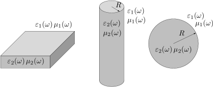
The unbounded DGFs for each individual dielectric material have to be joined at the common interface(s) across which the transverse field components of electric and magnetic fields have to be continuous. Let be a unit vector normal to the interface between two dielectrics. Then Maxwell’s equations imply that at the interface
| (547) | |||||
| (548) |
where the superscripts denote that the ource point connects to the ield point via a Green function . The dyadic Green function can then be decomposed into two parts, an unbounded DGF that represents direct propagation from to in an unbounded medium, and a scattering part that describes the contributions from multiply reflected and transmitted waves,
| (549) |
Mathematically speaking, the scattering part of the DGF has to be included in order to fix the boundary conditions at the medium interfaces, whereas the DGF of the unbounded medium is responsible for the correct boundary conditions at infinity.
A.4.1 Planarly layered media
There are two distinct methods for finding the dyadic Green function for planarly layered media. Here we will describe the Weyl expansion method [162, 41] that gives very compact expressions for the DGF. The second method using vector wave functions [163] is somewhat less transparent and will be reserved for cylindrically and spherically layered media.
The Weyl expansion is based on the translational invariance of the dyadic Green function with respect to the directions parallel to the planar interface,
| (550) |
[]. The matrix components for the scattering part of the DGF (we drop the superscript for notational convenience) associated with reflection from the interface are given by [162, 41]
| (551) | |||||
| (552) | |||||
| (553) | |||||
| (554) |
where and . The functions and are the Fresnel coefficients of - and -polarised waves,
| (555) |
The remaining vector components can be deduced by employing the replacement rule and the reciprocity theorem which translates into .
The Fresnel reflection coefficients (555) describe a single planar interface. For more than one interface, say a planar layer of thickness , the reflection coefficients can be combined (for both polarisations) as
| (556) |
where is the Fresnel coefficient for the interface between layers and .
The matrix components of the scattering DGF associated with transmission through the planar interface are
| (557) | |||||
| (558) | |||||
| (559) | |||||
| (560) | |||||
| (561) |
The transmission coefficients for - and -polarised waves are
| (562) |
The remaining vector components can again by symmetry arguments such as and , and .
A.4.2 Cylindrically layered media
For the two examples that follow here, we use the expansion of the DGF in terms of vector wave functions. We first define the cylindrical vector wave functions [164, 165] that depend on the radial () and axial () components of the wave number [] as
| (563) | |||||
The trigonometric functions have to be chosen appropriately for the ven and dd types of functions. In terms of those, the dyadic Green function for a cylindrical wire can be written in the form [164, 165]
| (565) | |||||
| (566) | |||||
| (567) | |||||
| (568) | |||||
In this compact notation, a superscript (1) means that the function in the respective vector wave function is a Hankel function of the first kind, . Without that superscript, it is understood that the Bessel function is used.
The reflection and transmission coefficients are determined by a -matrix equation
| (569) |
with
| (574) | |||||
| (579) |
and the abbreviations
| (580) |
With these preparations, the reflection and transmission coefficients can be derived as
| (587) | |||||
| (596) | |||||
| (603) | |||||
| (610) |
Note that, in contrast to planarly or spherically layered media, - and -polarised waves, represented by the and vector wave functions, becomes mixed for all angular momenta .
A.4.3 Spherically layered media
Similarly to the cylindrically layered case, we use the expansion of the dyadic Green function in terms of vector wave functions. The spherical vector wave functions are given by [166]
| (612) | |||||
With the help of those, the dyadic Green function for a dielectric sphere is [166]
| (613) | |||||
| (614) | |||||
| (615) | |||||
| (616) | |||||
For the following, it is convenient to define the Ricatti functions
| (617) |
In terms of those, the Mie scattering coefficients read
| (618) | |||||
| (619) |
| (620) | |||||
| (621) |
| (622) | |||||
| (623) |
| (624) | |||||
| (625) |
Note that the transmission coefficients can be further simplified by using the Wronski determinant between spherical Bessel and Hankel functions.
A.5 Born series expansion
In most situations, the geometric arrangement of dielectric bodies is not symmetrical enough to yield a separable Helmholtz operator in which case an expansion into vector wave functions would be feasible (Sec. A.4). Instead, we will describe an iterative method known from quantum mechanics and quantum field theory as Born (or Dyson) series expansion of the dyadic Green function. This method applies to an arbitrary arrangement of dielectric bodies but, in general, converges quickly only if the dielectric contrast between bodies and the surrounding material is sufficiently small.
Let us assume that from an arrangement of dielectric bodies, described by a dielectric permittivity , one can separate a part whose DGF is analytically known (e.g. vacuum, bulk material or layered media) and is described by a permittivity (see, for example, Fig. 37).
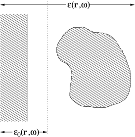
The dyadic Green functions are solutions to the respective Helmholtz equations
| (626) | |||||
| (627) |
Subtracting both equations from one another, we find that the difference between both DGFs [scattering Green function ] solves the inhomogeneous Helmholtz equation
| (628) |
where is the perturbation from the permittivity . Equation (A.5) bears some resemblance to the Helmholtz equation (521) for the electric field, with the current density being replaced by the rhs of Eq. (A.5). Its formal solution is therefore
| (629) |
Because the unknown scattering DGF appears on both sides of Eq. (629), making it a Fredholm integral equation of the second kind, one can solve it iteratively as [144]
| (630) | |||||
Equation (630) is known as the Born (or Dyson) series expansion of the scattering dyadic Green function . It has a simple diagrammatic representation as shown in Fig. 38.

The field propagates from the source point to the observation point via the intermediate positions . Each of the arrows represents the dyadic Green function (which we assumed to be analytically known), and each intermediate position (or vertex) carries a weight factor . The intermediate positions are integrated over, and the number of those points increases with the order of the iteration.
As the Born series (630) is a perturbation series in , it is clear that fast convergence is only guaranteed for small enough permittivity (or equivalently, refractive index) contrast. It should be noted, however, that the series does always eventually converge to its unique solution .
A.6 Local-field corrected Green tensors
While the DGF connects the macroscopic electric field with a macroscopic source [recall Eq. (522)], we are often interested in the coupling of the local electromagnetic field to microscopic sources such as atoms. For atoms which are embedded in a magnetoelectric medium, this difference between microscopic and macroscopic quantities leads to local-field corrections which can be implemented via the real-cavity model: One assumes that both field point and source point are not situated directly in the medium but surrounded by small free-space cavities of radius (cf. Fig. 39). Modifying the original permittivity and (inverse) permeability describing the present media to
| (631) |
the required local-field corrected DGF can be found as the solution to
| (632) |
The real-cavity model thus accounts for the fact that an atom occupies some space within the host medium, where the cavity radius is of the order of one half the lattice constant of the latter.
For magnetoelectrics (but not for metals), the condition is typically valid for the relevant frequencies of the electromagnetic field. In this case, the effect of the introduced cavities can be studied in a perturbative way by means of the spherical DGFs given in Sec. A.4.3. One finds that the local-field corrected single-point DGF is given by [167, 71]
| (633) |
where is the uncorrected DGF, denotes the permittvity of the unperturbed host medium at the source and field points (similarly for ) and is the respective refractive index. The first term in Eq. (633) represents contributions to the electric field which are reflected at the interior of the cavity and never reach the surrounding medium [type (i) in Fig. 39(a)]. The second term represents contributions which are transmitted into the host medium and, after possible transmissions and reflections, transmitted back into the cavity [type (ii)]; each of the transmissions through the cavity surface gives rise to one factor in round brackets. Processes where the field is backreflected from the outside of the cavity [type (iii)] have been neglected since they are of higher order in the small parameter .
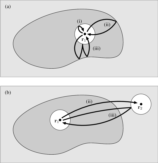
Similarly, the local-field corrected two-point DGF is found to be [71]
| (634) |
Equation (634) represents the transmission of the field out of the first cavity, transmissions and reflections within the host medium, followed by a transmission into the second cavity [type (ii) of Fig. 39(b)]; each of the transmissions at the cavity surfaces gives rise to one of the two factors. Again, reflections at the outside of either cavity have been neglected [type (iii)].
When describing magnetic interactions, the curl of the DGF typically arises. Local-field corrections in such situations cannot simply be obtained by taking the curl of Eqs. (633) and (634) above, since the implementation of the local-field correction via the real-cavity model does not commute with this vector operation. Instead, the local-field correction has to applied after taking the curl. One finds the single-point DGF [58]
| (635) |
and the two-point DGFs [58]
| (636) | |||
| (637) | |||
| (638) |
References
- [1] C. Itzykson and J.-B. Zuber: Quantum Field Theory, McGraw-Hill, Singapore 1980
- [2] M. Born and E. Wolf: Principles of Optics, Pergamon, London 1959
- [3] W. Vogel and D.-G. Welsch: Quantum Optics, Wiley-VCH, Weinheim 2006
- [4] L.D. Landau and E.M. Lifshitz: Electrodynamics of Continuous Media, Pergamon, London 1960
- [5] \referB. Yurke, S.L. McCall, J.R. Klauder Phys. Rev. A3319864033
- [6] \referS. Prasad, M.O. Scully, W. Martienssen Opt. Commun.621987139
- [7] \referZ.Y. Ou, C.K. Hong, L. MandelOpt. Commun. 631987118
- [8] \referH. Fearn, R. LoudonOpt. Commun. 641987485
- [9] \referR.A. Campos, B.E.A. Saleh, M.C. Teich Phys. Rev. A4013711989
- [10] \referU. LeonhardtPhys. Rev. A4819933265
- [11] R. Bhatia: Matrix analysis, Springer, New York 1997
- [12] H. Minc: Permanents, Addison–Welsey, Reading, MA 1978
- [13] S. Scheel: quant-ph/0406127 (2004)
- [14] S. Scheel: Conditional Linear Optical Networks, in Quantum Information Processing Chap. 28, ed. T. Beth and G. Leuchs, Wiley-VCH, Weinheim 2005
- [15] \referC.K. Hong, Z.Y. Ou, L. Mandel Phys. Rev. Lett.5919872044
- [16] \referH.B.G. CasimirProc. K. Ned. Akad. Wet.511948793
- [17] \referL.L. DeRaad Jr., K.A. MiltonAnn. Phys. (N.Y.)1361981229
- [18] \referT.H. BoyerPhys. Rev.17419681764
- [19] \referM. Babiker, E.A. Power, T. ThirunamachandranProc. R. Soc. Lond. A3381974235
- [20] \referE.A. Power, ZienauPhil. Trans. R. Soc. London Ser. A2511959427
- [21] \referR. G. WoolleyProc. R. Soc. London, Ser. A3211971557
- [22] D.P. Craig and T. Thirunamachandran: Molecular Quantum Electrodynamics, Academic Press, New York 1984
- [23] P.W. Milonni: The Quantum Vacuum, Academic Press, New York 1992
- [24] H.M. Nussenzveig: Causality and dispersion relations, Academic Press, New York 1972
- [25] \referE.T. Jaynes, F.W. CummingsProc. IEEE 51196389
- [26] S. Haroche: Cavity Quantum Electrodynamics in Fundamental Systems in Quantum Optics, Les Houches Summer School Session LIII, p. 767, ed. J. Dalibard, J.M. Raimond, J. Zinn-Justin, North-Holland, Amsterdam 1992
- [27] \referB.W. Shore, P.L. KnightJ. Mod. Opt. 4019931195
- [28] \referH. YamamotoAppl. Phys. A421987245
- [29] \referI. YanetkaPhysica B2701999371
- [30] \referB. Huttner, S.M. BarnettPhys. Rev. A4619924306
- [31] \referB. Huttner, S.M. BarnettEurophys. Lett.181992487
- [32] \referJ.J. HopfieldPhys. Rev.11219581555
- [33] L. Knöll, S. Scheel, and D.-G. Welsch: QED in dispersing and absorbing media, in Coherence and Statistics of Photons and Atoms, ed. J. Peřina, Wiley, New York 2001
- [34] \referU. FanoPhys. Rev.10319561202
- [35] \referE. Schmidt, J. Jeffers, S.M. Barnett, L. Knöll, D.-G. WelschJ. Mod. Opt.451997377
- [36] \referL.G. Suttorp, M. WubsPhys. Rev. A702004013816
- [37] D.B. Melrose and R.C. McPhedran: Electromagnetic Processes in Dispersive Media, Cambridge University Press, Cambridge 1991
- [38] \referC. Raabe, S. Scheel, D.-G. Welsch Phys. Rev. A752007053813
- [39] \referS. Scheel, L. Knöll, D.-G. WelschPhys. Rev. A581998700
- [40] \referHo Trung Dung, S.Y. Buhmann, L. Knöll, D.-G. Welsch, S. Scheel, J. KästelPhys. Rev. A682003043816
- [41] \referHo Trung Dung, L. Knöll, D.-G. WelschPhys. Rev. A5719983931
- [42] \referS.M. Barnett, C.R. Gilson, B. Huttner, N. ImotoPhys. Rev. Lett.7719961739
- [43] \referT. Gruner, D.-G. WelschPhys. Rev. A 5319961818
- [44] \referR. Matloob, R. LoudonPhys. Rev. A53 19964567
- [45] \referR. MatloobPhys. Rev. A60199950
- [46] \referO. DiStefano, S. Savasta, R. Girlanda Phys. Rev. A612000023803
- [47] \referL.G. SuttorpJ. Phys. A: Math. Theor 4020073697
- [48] \referJ.B. PendryPhys. Rev. Lett.8520003966
- [49] S.Y. Buhmann, S. Scheel: arXiv:0806.2211 (2008)
- [50] \referT. Gruner, D.-G. WelschPhys. Rev. A 5419961661
- [51] \referM. Khanbekyan, D.-G. Welsch, C. di Fidio, W. VogelPhys. Rev. A782008013822
- [52] \referL. Knöll, S. Scheel, E. Schmidt, D.-G. Welsch, A.V. ChizhovPhys. Rev. A5919994716
- [53] \referS. Scheel, L. Knöll, T. Opatrný, D.-G. WelschPhys. Rev. A622000043803
- [54] \referS. Scheel, D.-G. WelschPhys. Rev. A 642001063811
- [55] S. Scheel and D.-G. Welsch: Non-classical Gaussian states in noisy environments, in Quantum Information Processing Chap. 8, ed. T. Beth and G. Leuchs, Wiley-VCH, Weinheim 2005
- [56] \referG. Vidal, R.F. WernerPhys. Rev. A 652002032314
- [57] \referS.Y. Buhmann, L. Knöll, D.-G. Welsch, Ho Trung DungPhys. Rev. A702004052117
- [58] \referH. Safari, D.-G. Welsch, S.Y. Buhmann, S. ScheelPhys. Rev. A782008062901
- [59] M. Schubert and B. Wilhelmi: Nonlinear optics and quantum electronics, Wiley, New York 1986
- [60] \referS. Scheel, D.-G. WelschPhys. Rev. Lett. 962006073601
- [61] \referS. Scheel, D.-G. Welsch J. Phys. B: At. Mol. Opt. Phys.392006S711
- [62] \referS. Scheel, L. Knöll, D.-G. Welsch, S.M. BarnettPhys. Rev. A6019991590
- [63] \referS. Scheel, L. Knöll, D.-G. Welsch Phys. Rev. A6019994094
- [64] \referS. Scheel, L. Knöll, D.-G. Welsch Acta Phys. Slov.491999585
- [65] \referM.S. Yeung, T.K. GustafsonPhys. Rev. A 5519965227
- [66] \referJ.M. Wylie, J.E. SipePhys. Rev. A 3019841185
- [67] \referG. JuzeliūnasPhys. Rev. A551997R4015
- [68] \referM.S. Tomaš, Z. LenacPhys. Rev. A 5619974197
- [69] \referM. FleischhauerPhys. Rev. A 6019992534
- [70] \referR.J. Glauber, M. LewensteinPhys. Rev. A 431991467
- [71] \referHo Trung Dung, S.Y. Buhmann, D.-G. Welsch Phys. Rev. A742006023803
- [72] H.A. Bethe and E.E. Salpeter: Quantum Mechanics of One and Two-Electron Atoms, Springer, Berlin 1957
- [73] \referM. Altarelli, D.L. Dexter, H.M. Nussenzveig, D.Y. SmithPhys. Rev. B619724502
- [74] \referG. Frye, R.L. WarnockPhys. Rev.1301963478
- [75] \referS. ScheelPhys. Rev. A782008013841
- [76] \referS.M. Barnett, R. LoudonPhys. Rev. Lett. 7719962444
- [77] J. Brown and A. Carrington: Rotational Spectroscopy of Diatomic Molecules, Cambridge University Press, Cambridge 2003
- [78] \referS.Y. Buhmann, M.R. Tarbutt, S. Scheel, E.A. HindsPhys. Rev. A782008052901
- [79] \referN. Vanhaecke, O. DulieuMol. Phys. 10520071723
- [80] \referE.A. Hinds, I.A. HughesJ. Phys. D 321999R119
- [81] \referR. Folman, P. Krüger, J. Schmiedmayer, J. Denschlag, C. HenkelAdv. At. Mol. Opt. Phys.482002263
- [82] \referJ. Fortágh, C. Zimmermann Rev. Mod. Phys.792007235
- [83] \referA. Günther, M. Kemmler, S. Kraft, C.J. Vale, C. Zimmermann, J. FortághPhys. Rev. A712005063619
- [84] \referP.K. Rekdal, S. Scheel, P.L. Knight, E.A. Knight Phys. Rev. A702004013811
- [85] \referM.P.A. Jones, C.J. Vale, D. Sahagun, B.V. Hall, E.A. HindsPhys. Rev. Lett.912003080401
- [86] \referC. Henkel, S. Pötting, M. Wilkens Appl. Phys. B: Lasers Opt.B691999379
- [87] \referS. Scheel, P.K. Rekdal, P.L. Knight, E.A. HindsPhys. Rev. A722005042910
- [88] \referE.M. PurcellPhys. Rev.691946681
- [89] \referU. Hohenester, A. Eiguren, S. Scheel, E.A. HindsPhys. Rev. A762007033618
- [90] \referF. London, H. London Proc. R. Soc. London, Ser. A149193571
- [91] \referC.S. Gorter, H.B.G. CasimirZ. Phys. 351934963
- [92] \referE.M. LifshitzSov. Phys. JETP2195673
- [93] \referJ.E. Lennard–JonesTrans. Faraday Soc.281932333
- [94] \referH.B.G. Casimir, D. PolderPhys. Rev.731948360
- [95] \referF. LondonZ. Phys.631930245
- [96] \referS.Y. Buhmann, Ho Trung Dung, T. Kampf, D.-G. Welsch Eur. Phys. J. D35200515
- [97] \referS.Y. Buhmann, D.-G. WelschProg. Quantum Electron. 31200651
- [98] \referC. Henkel, K. Joulain, J. Mulet, J. Greffet J. Opt. A: Pure Appl. Opt.42002S109
- [99] J.D. van der Waals: Over de Continuiteit van den Gas- en Vloeistoftoestand (on the continuity of the gas and liquid state), Ph.D. thesis, Leiden 1873
- [100] J. Mahanty and B.W. Ninham: Dispersion Forces, Academic Press, London 1976
- [101] \referM. Bordag, U. Mohideen, V.M. Mostepanenko Phys. Rep.35320011
- [102] \referK.A. MiltonJ. Phys. A: Math. Gen.372004R209
- [103] \referS.K. LamoreauxRep. Prog. Phys.682005201
- [104] \referS.K. LamoreauxPhys. Today60200740
- [105] \referC. Raabe, D.-G. WelschPhys. Rev. A732006063822
- [106] \referC. Raabe, D.-G. WelschPhys. Rev. A712005013814
- [107] \referC. Raabe, L. Knöll, D.-G. Welsch Phys. Rev. A682003033810
- [108] \referE.A. HindsAdv. At. Mol. Opt. Phys.281991237
- [109] \referE.A. HindsAdv. At. Mol. Opt. Phys. Suppl.219941
- [110] \referA.D. McLachlanProc. R. Soc. Lond. Ser. A2711963387
- [111] \referG.S. AgarwalPhys. Rev. A111975243
- [112] \referJ. Schwinger, L.L. DeRaad Jr., K.A. MiltonAnn. Phys.115 19781
- [113] \referI.V. Bondarev, P. LambinPhys. Rev. B722005035451
- [114] \referA. Sambale, S.Y. Buhmann, D.-G. Welsch, M.S. Tomaš Phys. Rev. A752007042109
- [115] \referS.Y. Buhmann, T. Kampf, D.-G. WelschPhys. Rev. A 722005032112
- [116] \referM.J. Mehl, W.L. SchaichSurf. Sci.991980553
- [117] \referT.H. BoyerPhys. Rev.180196919
- [118] J.D. Jackson, Classical Electrodynamics, 3rd edn., Wiley, New York 1998
- [119] \referS. KryszewskiMol. Phys.7819931225
- [120] \referM.S. TomašPhys. Rev. A722005034104
- [121] \referY. Tikochinsky, L. SpruchPhys. Rev. A4819934236
- [122] \referS.Y. Buhmann, Ho Trung Dung, D.-G. Welsch J. Opt. B: Quantum Semiclass. Opt.62004S127
- [123] \referH. MargenauRev. Mod. Phys.1119391
- [124] H. Margenau and N.R. Kestner: Theory of Intermolecular Forces, Pergamon Press, Oxford 1969
- [125] \referG. Feinberg, J. SucherPhys. Rep.180198983
- [126] G. Compagno, R. Passante, F. Persico: Atom–Field Interactions and Dressed Atoms, Cambridge University Press, Cambridge 1995
- [127] \referA. SalamInt. Rev. Phys. Chem.272008405
- [128] \referA.D. McLachlanMol. Phys.71964381
- [129] \referJ. Mahanty, B.W. NinhamJ. Phys. A: Math. Gen.61973 1140
- [130] \referH. Safari, S.Y. Buhmann, D.-G. Welsch, Ho Trung Dung Phys. Rev. A742006042101
- [131] \referM.S. TomašJ. Phys. A: Math. Gen.3920066785
- [132] \referS. Spagnolo, D.A.R. Dalvit, P.W. MilonniPhys. Rev. A 752007052117
- [133] \referG. Feinberg, J. SucherJ. Chem. Phys.4819683333
- [134] \referG. Feinberg, J. SucherPhys. Rev. A219702395
- [135] \referC. Farina, F.C. Santos, A.C. TortAm. J. Phys.702002 421
- [136] \referC. Farina, F.C. Santos, A.C. TortJ. Phys. A: Math. Gen. 3520022477
- [137] \referE.A. Power, T. ThirunamachandranPhys. Rev. A251982 2473
- [138] \referS. Spagnolo, R. Passante, L. RizzutoPhys. Rev. A732006 062117
- [139] \referH. Safari, D.-G. Welsch, Ho Trung Dung, S.Y. Buhmann Phys. Rev. A772008053824
- [140] \referB.M. Axilrod, E. TellerJ. Chem. Phys.111943299
- [141] \referP.W. Milonni, P.B. LernerPhys. Rev. A4619921185
- [142] \referR. GolestanianPhys. Rev. Lett.952005230601
- [143] \referS.Y. Buhmann, H. Safari, D.-G. Welsch, Ho Trung Dung Open Syst. Inf. Dyn.132006427
- [144] \referS.Y. Buhmann, D.-G. WelschAppl. Phys. B822006189
- [145] \referE.A. Power, T. Thirunamachandran Proc. R. Soc. Lond. Ser. A4011985267
- [146] \referE.A. Power, T. ThirunamachandranPhys. Rev. A501994 3929
- [147] \referC. Henkel, K. JoulainEurophys. Lett.722005929
- [148] \referM.S. TomašPhys. Lett. A3422005381
- [149] \referS.Y. Buhmann, S. ScheelPhys. Rev. Lett. 1002008253201
- [150] \referI.E. Dzyaloshinskii, E.M. Lifshitz, L.P. PitaevskiiAdv. Phys.101961165
- [151] \referE. Hagley, X. Maître, G. Nogues, C. Wunderlich, M. Brune, J.M. Raimond, S. HarochePhys. Rev. Lett. 7919971
- [152] \referA. Kuhn, M. Hennrich, G. Rempe Phys. Rev. Lett.892002067901
- [153] \referJ. McKeever, A. Boca, A.D. Boozer, R. Miller, J.R. Buck, A. Kuzmich, H.J. Kimble Science30320041992
- [154] \referM. Khanbekyan, L. Knöll, A.A. Semenov, W. Vogel, D.-G. WelschPhys. Rev. A692004043807
- [155] \referG. Cui, M.G. RaymerOpt. Express1320059660
- [156] \referH. T. Dung, L. Knöll, D.-G. Welsch Phys. Rev. A622000053804
- [157] \referS. Götzinger, L. de S. Menezes, A. Mazzei, S. Kühn, V. Sandoghdar, O. BensonNanoletters620061151
- [158] \referH. T. Dung, L. Knöll, D.-G. Welsch Phys. Rev. A642001013804
- [159] \referH. T. Dung, S. Scheel, D.-G. Welsch, L. Knöll J. Opt. B: Quantum Semiklass. Opt.42002S169
- [160] P. Moon and D.E. Spencer: Field Theory Handbook, Including Coordinate Systems, Differential Equations, and Their Solutions, 2nd ed., Springer, New York 1988
- [161] W.C. Chew: Waves and Fields in Inhomogeneous Media, IEEE Press, New York 1994
- [162] \referM.S. TomašPhys. Rev. A5120002545
- [163] \referL.W. Li, P.S. Kooi, M.S. Leong, T.S. YeoJ. Electromagn. Waves Appl.81994663
- [164] C.T. Tai: Dyadic Green’s Functions in Electromagnetic Theory, IEEE Press, Piscataway, New Jersey 1991
- [165] \referL.W. Li, P.S. Kooi, M.S. Leong, T.S. YeoJ. Electromagn. Waves Appl.142000961
- [166] \referL.W. Li, P.S. Kooi, M.S. Leong, T.S. YeoIEEE Transactions on Microwave Theory and Techniques4219942302
- [167] \referM.S. TomašPhys. Rev. A632001053811