On the valuation of compositions in Lévy term structure models

Abstract.

We derive explicit valuation formulae for an exotic path-dependent interest rate derivative, namely an option on the composition of LIBOR rates. The formulae are based on Fourier transform methods for option pricing. We consider two models for the evolution of interest rates: an HJM-type forward rate model and a LIBOR-type forward price model. Both models are driven by a time-inhomogeneous Lévy process.

1. Introduction

The main aim of this paper is to derive simple and analytically tractable valuation formulae for an exotic path dependent interest rate derivative, namely an option on the composition of LIBOR rates. The formulae make use of Fourier transform techniques, see e.g. Eberlein, Glau, and Papapantoleon EberleinGlauPapapantoleon08, and the change-of-numeraire technique. There are two models for the term structure of interest rates considered in this paper: a Heath–Jarrow–Morton-type forward rate model and a LIBOR-type forward price model, both driven by a general time-inhomogeneous Lévy process.

A standard approach to modeling the term structure of interest rates is that of HeathJarrowMorton92. In the Heath–Jarrow–Morton (henceforth HJM) framework subject to modeling are instantaneous continuously compounded forward rates which are driven by a $d$-dimensional Wiener process. However, data from bond markets do not support the use of the normal distribution. Empirical evidence for the non-Gaussianity of daily returns from bond market data can be found in [chapter 5]Raible00; the fit of the normal inverse Gaussian distribution to the same data is particularly good, supporting the use of Lévy processes for modeling interest rates. Similar evidence appears in the risk-neutral world, i.e. from caplet implied volatility smiles and surfaces; see EberleinKluge04.

The Lévy forward rate model was developed in EberleinRaible99 and extended to time-inhomogeneous Lévy processes in Eberlein, Jacod, and Raible EberleinJacodRaible05. In these models, forward rates are driven by a (time-inhomogeneous) Lévy process; therefore, the model allows to accurately capture the empirical dynamics of interest rates, while it is still analytically tractable, so that closed form valuation formulae for liquid derivatives can be derived. Valuation formulae for caps, floors, swaptions and range notes have been derived in EberleinKluge04 EberleinKluge04,EberleinKluge05, while estimation and calibration methods are discussed in EberleinKluge04 EberleinKluge04,EberleinKluge06.

Moreover, EberleinJacodRaible05 provide a complete classification of all equivalent martingale measures in the Lévy forward rate model. They also prove that in certain situations – essentially, if the driving process is $1$-dimensional – the set of equivalent martingale measures becomes a singleton.

The main pitfall of the HJM framework is the assumption of continuously compounded rates, while in real markets interest accrues according to a discrete grid, the tenor structure. LIBOR market models, that is, arbitrage-free term structure models on a discrete tenor, were constructed in a series of articles by SandmannSondermannMiltersen95, MiltersenSandmannSondermann97, BraceGatarekMusiela97, and Jamshidian97. In addition, LIBOR market models are consistent with the market practice of pricing caps and floors using Black’s formula (cf. Black76).

Nevertheless, a familiar phenomenon appears: since the model is driven by a Brownian motion, it cannot be calibrated accurately to the whole term structure of volatility smiles. As a remedy, EberleinOezkan05 developed a LIBOR model driven by time inhomogeneous Lévy processes. Valuation methods for caps and floors, using approximation arguments, were presented in EberleinOezkan05 and Kluge05, while calibration issues for this model are discussed in EberleinKluge06.

The Lévy forward price model is a market model based on the forward price – rather than the LIBOR rate – and driven by time inhomogeneous Lévy processes; it was put forward by EberleinOezkan05 (2005, pp. 342–343). A detailed construction of the model is presented in Kluge05 (2005, Chapter 3); there, it is also shown how this model can be embedded in the Lévy forward rate model.

Although the forward LIBOR rate and the forward price differ only by an additive and a multiplicative constant, the two specifications lead to models with very different qualitative and quantitative behavior. In the LIBOR model, LIBOR rates change by an amount relative to their current level, while in the forward price model changes do not depend on the actual level (cf. [p. 60]Kluge05). There are authors who claim that models based on the forward process – also coined “arithmetic” or “Bachelier” LIBOR models – are able to better describe the dynamics of the market than (log-normal) LIBOR market models; see Henrard05.

Another advantage of the forward price model is that the driving process remains a time-inhomogeneous Lévy process under each forward measure, hence this model is particularly suitable for practical implementation. The downside is that negative LIBOR rates can occur, like in an HJM model.

This paper is organized as follows: in section 2 we review some basic properties of the driving time-inhomogeneous Lévy processes and in section 3 we describe the forward rate and forward price frameworks for modeling the term structure of interest rates. In section 4 the payoff of the option on the composition is described and valuation formulae are derived in the two modeling frameworks. Finally, section 5 concludes.

2. Time-inhomogeneous Lévy processes

Let ($\Omega,\mathcal{F},\mathrm{I\kern-1.99997ptF},\mathrm{I\kern-1.99997ptP}$) be a complete stochastic basis, where $\mathcal{F}=\mathcal{F}_{T^{*}}$ and the filtration $\mathrm{I\kern-1.99997ptF}=(\mathcal{F}_{t})_{t\in[0,T^{*}]}$ satisfies the usual conditions; we assume that $T^{*}\in\mathbb{R}_{+}$ is a finite time horizon. The driving process $L=(L_{t})_{t\in[0,T^{*}]}$ is a time-inhomogeneous Lévy process, or a process with independent increments and absolutely continuous characteristics, in the sequel abbreviated PIIAC. Therefore, $L$ is an adapted, càdlàg, real-valued stochastic process with independent increments, starting from zero, where the law of $L_{t}$, $t\in[0,T^{*}]$, is described by the characteristic function

$$\mathrm{I\kern-1.99997ptE}\left[\mathrm{e}^{iuL_{t}}\right]=\exp\int_{0}^{t}\bigg{(}ib_{s}u-\frac{c_{s}}{2}u^{2}+\int_{\mathbb{R}}(\mathrm{e}^{iux}-1-iux)\lambda_{s}(\mathrm{d}x)\bigg{)}\mathrm{d}s,$$ (2.1)

where $b_{t}\in\mathbb{R}$, $c_{t}\in\mathbb{R}_{+}$ and $\lambda_{t}$ is a Lévy measure, i.e. it satisfies $\lambda_{t}(\{0\})=0$ and $\int_{\mathbb{R}}(1\wedge|x|^{2})\lambda_{t}(\mathrm{d}x)<\infty$, for all $t\in[0,T^{*}]$. In addition, the process $L$ satisfies Assumptions ($\mathbb{AC}$) and ($\mathbb{EM}$) given below.

Assumption ($\mathbb{AC}$).

The triplets ($b_{t},c_{t},\lambda_{t}$) satisfy

$$\int_{0}^{T^{*}}\bigg{(}|b_{t}|+c_{t}+\int_{\mathbb{R}}(1\wedge|x|^{2})\lambda_{t}(\mathrm{d}x)\bigg{)}\mathrm{d}t<\infty.$$ (2.2)

Assumption ($\mathbb{EM}$).

There exist constants $M,\varepsilon>0$ such that for every $u\in[-(1+\varepsilon)M,(1+\varepsilon)M]$

$$\int_{0}^{T^{*}}\int_{\{|x|>1\}}\exp(ux)\lambda_{t}(\mathrm{d}x)\mathrm{d}t<\infty.$$ (2.3)

Moreover, without loss of generality, we assume that $\int_{\{|x|>1\}}\mathrm{e}^{ux}\lambda_{t}(\mathrm{d}x)<\infty$ for all $t\in[0,T^{*}]$ and all $u\in[-(1+\varepsilon)M,(1+\varepsilon)M]$.

These assumptions render the process $L=(L_{t})_{0\leq t\leq T^{*}}$ a special semimartingale, therefore it has the canonical decomposition (cf. Jacod and Shiryaev [II.2.38]JacodShiryaev03, and EberleinJacodRaible05)

$$L_{t}=\int_{0}^{t}b_{s}\mathrm{d}s+\int_{0}^{t}\sqrt{c_{s}}\mathrm{d}W_{s}+\int_{0}^{t}\int_{\mathbb{R}}x(\mu^{L}-\nu)(\mathrm{d}s,\mathrm{d}x),$$ (2.4)

where $\mu^{L}$ is the random measure of jumps of the process $L$ and $W=(W_{t})_{0\leq t\leq T^{*}}$ is a $\mathrm{I\kern-1.99997ptP}$-standard Brownian motion. The triplet of predictable or semimartingale characteristics of $L$ with respect to the measure $P$, $\mathbb{T}(L|P)=(B,C,\nu)$, is

$$B_{t}=\int_{0}^{t}b_{s}\mathrm{d}s, C_{t}=\int_{0}^{t}c_{s}\mathrm{d}s,\quad\nu([0,t]\times A)=\int_{0}^{t}\int_{A}\lambda_{s}(\mathrm{d}x)\mathrm{d}s,$$ (2.5)

where $A\in\mathcal{B}(\mathbb{R})$. The triplet ($b,c,\lambda$) represents the local or differential characteristics of $L$. In addition, the triplet of semimartingale characteristics ($B,C,\nu$) determines the distribution of $L$.

We denote by $\theta_{s}$ the cumulant generating function (i.e. the logarithm of the moment generating function) associated with the infinitely divisible distribution with Lévy triplet ($b_{s},c_{s},\lambda_{s}$), i.e. for $z\in[-(1+\varepsilon)M,(1+\varepsilon)M]$

$$\theta_{s}(z):=b_{s}z+\frac{c_{s}}{2}z^{2}+\int_{\mathbb{R}}(\mathrm{e}^{zx}-1-zx)\lambda_{s}(\mathrm{d}x).$$ (2.6)

Subject to Assumption $(\mathbb{EM})$, $\theta_{s}$ is well defined and can be extended to the complex domain $\mathbb{C}$, for $z\in\mathbb{C}$ with $\Re z\in[-(1+\varepsilon)M,(1+\varepsilon)M]$ and the characteristic function of $L_{t}$ can be written as

$$\mathrm{I\kern-1.99997ptE}\left[\mathrm{e}^{iuL_{t}}\right]=\exp\int_{0}^{t}\theta_{s}(iu)\mathrm{d}s.$$ (2.7)

If $L$ is a (time-homogeneous) Lévy process, then ($b_{s},c_{s},\lambda_{s}$) and thus also $\theta_{s}$ do not depend on $s$, and $\theta$ equals the cumulant generating function of $L_{1}$.

Lemma 2.1.

Let $L=(L_{t})_{0\leq t\leq T^{*}}$ be a time-inhomogeneous Lévy process satisfying assumption $(\mathbb{EM})$ and $f:\mathbb{R}_{+}\rightarrow\mathbb{C}$ a continuous function such that $|\Re(f)|\leq M$. Then

$$\mathrm{I\kern-1.99997ptE}\Bigg{[}\exp\int_{0}^{t}f(s)\mathrm{d}L_{s}\Bigg{]}=\exp\int_{0}^{t}\theta_{s}\big{(}f(s)\big{)}\mathrm{d}s.$$ (2.8)

(The integrals are to be understood componentwise for real and imaginary part.)

Proof.

The proof is similar to the proof of Lemma 3.1 in Eberlein and Raible EberleinRaible99; see also [Proposition 1.9]Kluge05. ∎

3. Lévy term structure models

In this section we review two approaches to modeling the term structure of interest rates, where the driving process is a time-inhomogeneous Lévy process.

3.1. The Lévy forward rate model

In the Lévy forward rate framework for modeling the term structure of interest rates, the dynamics of forward rates are specified and the prices of zero coupon bonds are then deduced. Let $T^{*}$ be a fixed time horizon and assume that for every $T\in[0,T^{*}]$, there exists a zero coupon bond maturing at $T$ traded in the market; in addition, let $U\in[0,T^{*}]$.

The forward rates are driven by a time-inhomogeneous Lévy process $L=(L_{t})_{t\in[0,T^{*}]}$ on the stochastic basis $(\Omega,\mathcal{F},\mathrm{I\kern-1.99997ptF},\mathrm{I\kern-1.99997ptP})$ with semimartingale characteristics ($B,C,\nu$) or local characteristics $(b,c,\lambda)$. The dynamics of the instantaneous continuously compounded forward rates for $T\in[0,T^{*}]$ is given by

$$f(t,T)=f(0,T)+\int_{0}^{t}\alpha(s,T)\mathrm{d}s-\int_{0}^{t}\sigma(s,T)\mathrm{d}L_{s},\quad 0\leq t\leq T.$$ (3.1)

The initial values $f(0,T)$ are deterministic, and bounded and measurable in $T$. In general, $\alpha$ and $\sigma$ are real-valued stochastic processes defined on $\Omega\times[0,T^{*}]\times[0,T^{*}]$ that satisfy the following conditions:

(A1):

for $s>T$ we have $\alpha(\omega;s,T)=0$ and $\sigma(\omega;s,T)=0$.

(A2):

$(\omega,s,T)\mapsto\alpha(\omega;s,T),\sigma(\omega;s,T)$ are $\mathcal{P}\otimes\mathcal{B}([0,T^{*}])$-measurable.

(A3):

$S(\omega):=\sup_{s,T\leq T^{*}}(|\alpha(\omega;s,T)|+|\sigma(\omega;s,T)|)<\infty$.

Then, (3.1) is well defined and we can find a “joint” version of all $f(t,T)$ such that $(\omega;t,T)\mapsto f(t,T)(\omega)1_{\{t\leq T\}}$ is $\mathcal{O}\otimes\mathcal{B}([0,T^{*}])$-measurable. Here $\mathcal{P}$ and $\mathcal{O}$ denote the predictable and optional $\sigma$-fields on $\Omega\times[0,T^{*}]$.

Taking the dynamics of the forward rates as the starting point, explicit expressions for the dynamics of zero coupon bond prices and the money market account can be deduced (cf. Proposition 5.2 in BjoerkDimasiKabanovRunngaldier97). From [(2.6)]EberleinKluge05, we get that the time-$T$ price of a zero coupon bond maturing at time $U$ is

$$B(T,U) =\frac{B(0,U)}{B(0,T)}\exp\left(\int_{0}^{T}\Sigma(s,T,U)\mathrm{d}L_{s}-\int_{0}^{T}A(s,T,U)\mathrm{d}s\right),$$ (3.2)

where the following abbreviations are used:

$$\Sigma(s,T,U) :=\Sigma(s,U)-\Sigma(s,T),$$

$$A(s,T,U) :=A(s,U)-A(s,T),$$

and

$$A(s,T):=\int_{s\wedge T}^{T}\alpha(s,u)\mathrm{d}u\quad\mathrm{and}\quad\Sigma(s,T):=\int_{s\wedge T}^{T}\sigma(s,u)\mathrm{d}u.$$

Similarly, using [(2.5)]EberleinKluge05, we have for the money market account

$$B_{T}^{M} =\frac{1}{B(0,T)}\exp\left(\int_{0}^{T}A(s,T)\mathrm{d}s-\int_{0}^{T}\Sigma(s,T)\mathrm{d}L_{s}\right).$$ (3.3)

In the sequel we will consider only deterministic volatility structures. Therefore, $\Sigma$ and $A$ are assumed to be deterministic real-valued functions defined on $\Delta:=\{(s,T)\in[0,T^{*}]\times[0,T^{*}];s\leq T\}$, whose paths are continuously differentiable in the second variable. Moreover, they satisfy the following conditions.

(B1):

The volatility structure $\Sigma$ is continuous in the first argument and bounded in the following way: for $(s,T)\in\Delta$ we have

$$0\leq\Sigma(s,T)\leq M,$$

where $M$ is the constant from Assumption ($\mathbb{EM}$). Furthermore, we have that $\Sigma(s,T)\neq 0$ for $s<T$ and $\Sigma(T,T)=0$ for $T\in[0,T^{*}]$.

(B2):

The drift coefficients $A(\cdot,T)$ are given by

$$A(s,T)=\theta_{s}(\Sigma(s,T)),$$ (3.4)

where $\theta_{s}$ is the cumulant generating function associated with the triplet $(b_{s},c_{s},\lambda_{s})$, $s\in[0,T]$.

Remark 3.1.

The drift condition (3.4) guarantees that bond prices discounted by the money market account are martingales; hence, $\mathrm{I\kern-1.99997ptP}$ is a martingale measure. In addition, from Theorem 6.4 in EberleinJacodRaible05, we know that the martingale measure is unique.

3.2. The Lévy forward price model

In the Lévy forward price model the dynamics of forward prices, i.e. ratios of successive bond prices, are specified. Let $0=T_{0}<T_{1}<\cdots<T_{N}<T_{N+1}=T^{*}$ denote a discrete tenor structure where $\delta_{i}=T_{i+1}-T_{i}$, $i\in\{0,1,\dots,N\}$; the model is constructed via backward induction, hence we denote by $T_{j}^{*}:=T_{N+1-j}$ for $j\in\{0,1,\dots,N+1\}$ and $\delta^{*}_{j}:=\delta_{N+1-j}$ for $j\in\{1,\dots,N+1\}$.

Consider a complete stochastic basis $(\Omega,\mathcal{F},\mathrm{I\kern-1.99997ptF},\mathrm{I\kern-1.99997ptP}_{T^{*}})$ and let $L=(L_{t})_{t\in[0,T^{*}]}$ be a time-inhomogeneous Lévy process satisfying Assumption $(\mathbb{EM})$. $L$ has semimartingale characteristics ($0,C,\nu^{T^{*}}$) or local characteristics $(0,c,\lambda^{T^{*}})$ and its canonical decomposition is

$$L_{t}=\int_{0}^{t}\sqrt{c_{s}}\mathrm{d}W_{s}^{T^{*}}+\int_{0}^{t}\int_{\mathbb{R}}x(\mu^{L}-\nu^{T^{*}})(\mathrm{d}s,\mathrm{d}x),$$ (3.5)

where $W^{T^{*}}$ is a $\mathrm{I\kern-1.99997ptP}_{T^{*}}$-standard Brownian motion, $\mu^{L}$ is the random measure associated with the jumps of $L$ and $\nu^{T^{*}}$ is the $\mathrm{I\kern-1.99997ptP}_{T^{*}}$-compensator of $\mu^{L}$. Moreover, we assume that the following conditions are in force.

(FP1):

For any maturity $T_{i}$ there exists a bounded, continuous, deterministic function $\eta(\cdot,T_{i}):[0,T_{i}]\rightarrow\mathbb{R}$, which represents the volatility of the forward price process $F(\cdot,T_{i},T_{i}+\delta_{i})$. Moreover, we require that the volatility structure satisfies

$$\Big{|}\sum_{k=1}^{i}\eta(s,T_{k})\Big{|}\leq M, \qquad\forall\;i\in\{1,\dots,N\},$$

for all $s\in[0,T^{*}]$, where $M$ is the constant from Assumption ($\mathbb{EM}$) and $\eta(s,T_{i})=0$ for all $s>T_{i}$.

(FP2):

The initial term structure $B(0,T_{i})$, $1\leq i\leq N+1$ is strictly positive. Consequently, the initial term structure of forward price processes is given, for $1\leq i\leq N$, by

$$F(0,T_{i},T_{i}+\delta_{i})=\frac{B(0,T_{i})}{B(0,T_{i}+\delta_{i})}.$$

The construction starts by postulating that the dynamics of the forward process with the longest maturity $F(\cdot,T_{1}^{*},T^{*})$ are driven by the time-inhomogeneous Lévy process $L$, and evolve as a martingale under the terminal forward measure $\mathrm{I\kern-1.99997ptP}_{T^{*}}$. Then, the dynamics of the forward processes for the preceding maturities are constructed by backward induction; therefore, they are driven by the same process $L$ and evolve as martingales under their associated forward measures.

Let us denote by $\mathrm{I\kern-1.99997ptP}_{T^{*}_{j-1}}$ the forward measure associated with the settlement date $T^{*}_{j-1}$, $j\in\{1,\dots,N+1\}$. The dynamics of the forward price process $F(\cdot,T^{*}_{j},T^{*}_{j-1})$ is given by

$$F(t,T^{*}_{j}\!,T^{*}_{j-1})\!=\!F(0,T^{*}_{j}\!,T^{*}_{j-1})\exp\!\left(\int_{0}^{t}b(s,T^{*}_{j}\!,T^{*}_{j-1})\mathrm{d}s\!+\!\!\int_{0}^{t}\!\eta(s,T^{*}_{j})\mathrm{d}L^{T^{*}_{j-1}}_{s}\!\right)$$

where

$$L^{T^{*}_{j-1}}_{t} =\int_{0}^{t}\sqrt{c_{s}}\mathrm{d}W^{T^{*}_{j-1}}_{s}+\int_{0}^{t}\int_{\mathbb{R}}x(\mu^{L}-\nu^{T^{*}_{j-1}})(\mathrm{d}s,\mathrm{d}x)$$

is a time-inhomogeneous Lévy process. Here $W^{T^{*}_{j-1}}$ is a $\mathrm{I\kern-1.99997ptP}_{T^{*}_{j-1}}$-standard Brownian motion and $\nu^{T^{*}_{j-1}}$ is the $\mathrm{I\kern-1.99997ptP}_{T^{*}_{j-1}}$-compensator of $\mu^{L}$. The forward price process evolves as a martingale under its corresponding forward measure, hence, we specify the drift of the forward price process to be

$$b(s,T^{*}_{j},T^{*}_{j-1}) =-\frac{1}{2}(\eta(s,T^{*}_{j}))^{2}c_{s}$$

$$\quad\;-\int_{\mathbb{R}}\left(\mathrm{e}^{\eta(s,T^{*}_{j})x}-1-\eta(s,T^{*}_{j})x\right)\lambda_{s}^{T^{*}_{j-1}}(\mathrm{d}x).$$ (3.6)

The forward measure $\mathrm{I\kern-1.99997ptP}_{T^{*}_{j-1}}$, which is defined on $(\Omega,\mathcal{F},(\mathcal{F}_{t})_{0\leq t\leq T^{*}_{j-1}})$, is related to the terminal forward measure $\mathrm{I\kern-1.99997ptP}_{T^{*}}$ via

$$\frac{\mathrm{d}\mathrm{I\kern-1.99997ptP}_{T^{*}_{j-1}}}{\mathrm{d}\mathrm{I\kern-1.99997ptP}_{T^{*}}}=\prod_{k=1}^{j-1}\frac{F(T^{*}_{j-1},T^{*}_{k},T_{k-1}^{*})}{F(0,T_{k}^{*},T^{*}_{k-1})}=\frac{B(0,T^{*})}{B(0,T_{j-1}^{*})}\prod_{k=1}^{j-1}F(T^{*}_{j-1},T^{*}_{k},T_{k-1}^{*}).$$

In addition, the $\mathrm{I\kern-1.99997ptP}_{T^{*}_{j-1}}$-Brownian motion is related to the $\mathrm{I\kern-1.99997ptP}_{T^{*}}$-Brownian motion via

$$W_{t}^{T^{*}_{j-1}} =W_{t}^{T^{*}_{j-2}}-\int_{0}^{t}\eta(s,T^{*}_{j-1})\sqrt{c_{s}}\mathrm{d}s=\dots$$

$$=W_{t}^{T^{*}}-\int_{0}^{t}\left(\sum_{k=1}^{j-1}\eta(s,T^{*}_{k})\right)\sqrt{c_{s}}\mathrm{d}s.$$ (3.7)

Similarly, the $\mathrm{I\kern-1.99997ptP}_{T^{*}_{j-1}}$-compensator of $\mu^{L}$ is related to the $\mathrm{I\kern-1.99997ptP}_{T^{*}}$-compensator of $\mu^{L}$ via

$$\nu^{T^{*}_{j-1}}(\mathrm{d}s,\mathrm{d}x) =\exp\Big{(}\eta(s,T^{*}_{j-1})x\Big{)}\nu^{T^{*}_{j-2}}(\mathrm{d}s,\mathrm{d}x)=\dots$$

$$=\exp\left(x\sum_{k=1}^{j-1}\eta(s,T^{*}_{k})\right)\nu^{T^{*}}(\mathrm{d}s,\mathrm{d}x).$$ (3.8)

Remark 3.2.

The process $L=L^{T^{*}}$, driving the most distant forward price, and $L^{T^{*}_{j-1}}$, driving the forward price $F(\cdot,T^{*}_{j},T^{*}_{j-1})$, are both time-inhomogeneous Lévy processes, sharing the same martingale parts and differing only in the finite variation parts. Applying Girsanov’s theorem for semimartingales yields that the $\mathrm{I\kern-1.99997ptP}_{T^{*}_{j-1}}$-finite variation part of $L$ is

$$\int_{0}^{\cdot}c_{s}\left(\sum_{k=1}^{j-1}\eta(s,T^{*}_{k})\right)\mathrm{d}s+\int_{0}^{\cdot}\int_{\mathbb{R}}x\left(\exp\Big{(}x\sum_{k=1}^{j-1}\eta(s,T^{*}_{k})\Big{)}-1\right)\nu^{T^{*}}(\mathrm{d}s,\mathrm{d}x).$$

4. Valuation of options on compositions

Consider a discrete tenor structure $0=T_{0}<T_{1}<\cdots<T_{N}<T_{N+1}=T^{*}$, where the accrual factor for the time period $[T_{i},T_{i+1}]$ is $\delta_{i}=T_{i+1}-T_{i}$, $i\in\{0,1,\dots,N\}$ and let $L(s_{i},T_{i})$ denote the time-$s_{i}$ forward LIBOR for the time period $[T_{i},T_{i+1}]$. The composition pays a floating rate, typically the LIBOR, compounded on several consecutive dates. The rates are fixed at the dates $s_{i}\leq T_{i}$ and the value of the composition is

$$\prod_{i=1}^{N}\big{(}1+\delta_{i}L(s_{i},T_{i})\big{)};$$

therefore, the composition equals an investment of one currency unit at the LIBOR rate for $N$ consecutive periods. The value of the composition is subjected to a cap (or floor) denoted by $K$ and is settled in arrears, at time $T^{*}$. Hence, a cap on the composition pays off at maturity the excess of the composition over $K$, i.e.

$$\left(\prod_{i=1}^{N}\big{(}1+\delta_{i}L(s_{i},T_{i})\big{)}-K\right)^{+},$$

and similarly, the payoff of a floor on the composition is

$$\left(K-\prod_{i=1}^{N}\big{(}1+\delta_{i}L(s_{i},T_{i})\big{)}\right)^{+}.$$

Notice that without the cap (resp. floor), the payoff of the composition would simply be that of a floating rate note, where the proceeds are reinvested. Similarly, if we only consider a single compounding date, then we are dealing with a caplet (resp. floorlet), with strike $\mathscr{K}:=\frac{K-1}{\delta}$.

In the following sections, we present methods for the valuation of a cap on the composition in the Lévy-driven forward rate and forward price frameworks. The value of a floor on the composition can either be deduced via analogous valuation formulae or via the cap-floor parity for compositions, which reads

$$\mathbf{C}(T^{*};K)=\mathbf{F}(T^{*};K)+B(0,T_{1})-KB(0,T^{*}).$$

Here $\mathbf{C}(T^{*};K)$ and $\mathbf{F}(T^{*};K)$ denote the time-$T_{0}$ value of a cap, resp. floor, on the composition with cap, resp. floor, equal to $K$.

4.1. Forward rate framework

In this section we derive an explicit formula for the valuation of a cap on the composition in the Lévy forward rate model, making use of the methods developed in EberleinGlauPapapantoleon08. As a special case, we get valuation formulae for caplets in the Lévy forward rate framework that generalize the results of EberleinKluge04, since we do not require the existence of a Lebesgue density (which is essential in the convolution representation of option prices; cf. [Chapter 3]Raible00).

Firstly, we calculate the quantity that appears in the composition. By an elementary calculation, we have that

$$\frac{B(s_{i},T_{i})}{B(s_{i},T_{i+1})}=\frac{B(0,T_{i})}{B(0,T_{i+1})}\exp\left(\int_{0}^{s_{i}}A(s,T_{i},T_{i+1})\mathrm{d}s-\int_{0}^{s_{i}}\Sigma(s,T_{i},T_{i+1})\mathrm{d}L_{s}\right)\!\!.$$

Using the fact that $1+\delta_{i}L(s_{i},T_{i})=\frac{B(s_{i},T_{i})}{B(s_{i},T_{i+1})}$ we immediately get

$$\prod_{i=1}^{N}\!\big{(}1\!+\!\delta_{i}L(s_{i},T_{i})\big{)}\! =\prod_{i=1}^{N}\frac{B(s_{i},T_{i})}{B(s_{i},T_{i+1})}$$

$$=\frac{B(0,T_{1})}{B(0,T^{*})}$$

$$\times\exp\!\left(\sum_{i=1}^{N}\int_{0}^{s_{i}}A(s,T_{i},T_{i+1})\mathrm{d}s\!-\!\sum_{i=1}^{N}\int_{0}^{s_{i}}\Sigma(s,T_{i},T_{i+1})\mathrm{d}L_{s}\right)\!\!.$$

Next, we define the forward measure associated with the date $T^{*}$ via the Radon–Nikodym derivative

$$\frac{\mathrm{d}\mathrm{I\kern-1.99997ptP}_{T^{*}}}{\mathrm{d}\mathrm{I\kern-1.99997ptP}} :=\frac{1}{B^{M}_{T^{*}}B(0,T^{*})}$$

$$\phantom{:}=\exp\left(-\int_{0}^{T^{*}}A(s,T^{*})\mathrm{d}s+\int_{0}^{T^{*}}\Sigma(s,T^{*})\mathrm{d}L_{s}\right).$$

The measures $\mathrm{I\kern-1.99997ptP}$ and $\mathrm{I\kern-1.99997ptP}_{T^{*}}$ are equivalent, since the density is strictly positive; moreover, we immediately note that $\mathrm{I\kern-1.99997ptE}\big{[}\frac{1}{B^{M}_{T^{*}}B(0,T^{*})}\big{]}=1$. The density process related to the change of measure is given by the restriction of the Radon–Nikodym derivative to the $\sigma$-field $\mathcal{F}_{t}$, $t\leq T^{*}$, therefore

$$\mathrm{I\kern-1.99997ptE}\left[\frac{\mathrm{d}\mathrm{I\kern-1.99997ptP}_{T^{*}}}{\mathrm{d}\mathrm{I\kern-1.99997ptP}}\Big{|}\mathcal{F}_{t}\right] =\frac{B(t,T^{*})}{B^{M}_{t}B(0,T^{*})}$$

$$=\exp\left(-\int_{0}^{t}A(s,T^{*})\mathrm{d}s+\int_{0}^{t}\Sigma(s,T^{*})\mathrm{d}L_{s}\right).$$

This allows us to determine the tuple of functions that characterize the process $L$ under this change of measure and we can conclude, using Theorems III.3.24 and II.4.15 in JacodShiryaev03, that the driving process $L=(L_{t})_{t\in[0,T^{*}]}$ remains a time-inhomogeneous Lévy process under the measure $\mathrm{I\kern-1.99997ptP}_{T^{*}}$.

According to the first fundamental theorem of asset pricing the price of an option on the composition is equal to its discounted expected payoff under the martingale measure. Combined with the forward measure defined above, this gives

$$\mathbf{C}(T^{*};K) =\mathrm{I\kern-1.99997ptE}_{\mathrm{I\kern-1.39998ptP}}\left[\frac{1}{B^{M}_{T^{*}}}\left(\prod_{i=1}^{N}\frac{B(s_{i},T_{i})}{B(s_{i},T_{i+1})}-K\right)^{+}\right]$$

$$=B(0,T^{*})\mathrm{I\kern-1.99997ptE}_{\mathrm{I\kern-1.39998ptP}_{T^{*}}}\left[\left(\prod_{i=1}^{N}\frac{B(s_{i},T_{i})}{B(s_{i},T_{i+1})}-K\right)^{+}\right]$$

$$=B(0,T^{*})\mathrm{I\kern-1.99997ptE}_{\mathrm{I\kern-1.39998ptP}_{T^{*}}}\left[\left(\exp H-K\right)^{+}\right],$$

where the random variable $H$ is defined as

$$H:=\log\frac{B(0,T_{1})}{B(0,T^{*})}+\sum_{i=1}^{N}\int_{0}^{s_{i}}A(s,T_{i},T_{i+1})\mathrm{d}s-\sum_{i=1}^{N}\int_{0}^{s_{i}}\Sigma(s,T_{i},T_{i+1})\mathrm{d}L_{s}.$$

Let us denote by $M^{T^{*}}_{H}$ the moment generating function of $H$ under the measure $\mathrm{I\kern-1.99997ptP}_{T^{*}}$. The next theorem provides an analytical expression for the value of a cap on the composition. Preceding that, we provide an expression for $M^{T^{*}}_{H}(z)$ for suitable complex arguments $z$.

Lemma 4.1.

Let $M$ and $\varepsilon$ be suitably chosen such that $\Sigma(s,T)\leq M^{\prime}$ for all $s,T\in[0,T^{*}]$ and $\Sigma(s,T_{i+1})1_{[s_{i},s_{i+1}]}(s)\leq M^{\prime\prime}$ for all $s,s_{i},T_{i+1}\in[0,T^{*}]$, where $0<M^{\prime\prime}<M^{\prime}<M$ and $\frac{M}{M^{\prime\prime}}>N+1$. Then, for each $R\in\mathcal{I}_{2}=[1-\frac{M-M^{\prime\prime}(N+1)}{M^{\prime}+M^{\prime\prime}(N+1)},1+\frac{M-M^{\prime\prime}(N+1)}{M^{\prime}+M^{\prime\prime}(N+1)}]$, we have that $M^{T^{*}}_{H}(R)<\infty$ and for every $z\in\mathbb{C}$ with $\Re z=R$

$$M^{T^{*}}_{H}(z) =\mathcal{Z}^{z}\exp\left(\int_{0}^{T^{*}}\left(z\sum^{N}_{i=1}A(s,T_{i},T_{i+1})1_{[0,s_{i}]}(s)-\theta_{s}\Big{(}\Sigma(s,T^{*})\Big{)}\right.\right.$$

$$\qquad\qquad\left.\phantom{\int_{0}^{T^{*}}}\left.+\theta_{s}\Big{(}\Sigma(s,T^{*})-z\sum^{N}_{i=1}\Sigma(s,T_{i},T_{i+1})1_{[0,s_{i}]}(s)\Big{)}\right)\mathrm{d}s\right)$$

where $\mathcal{Z}:=\frac{B(0,T_{1})}{B(0,T^{*})}$.

Proof.

Fix an $R\in\mathcal{I}_{2}$. Then, for $z\in\mathbb{C}$ with $\Re z=R$, and denoting by $\underline{\overline{\Sigma}}(s,T)=\sum_{i=0}^{N}\Sigma(s,T_{i+1})1_{[s_{i},s_{i+1}]}(s)$, we get that

$$\Big{|}\Re\Big{(}-z\sum^{N}_{i=1}\Sigma(s,T_{i},T_{i+1})1_{[0,s_{i}]}(s)\Big{)}+\Sigma(s,T^{*})\Big{|}$$ (4.1)

$$= \Big{|}\Re\Big{(}z\sum_{i=0}^{N}\Sigma(s,T_{i+1})1_{[s_{i},s_{i+1}]}(s)-z\Sigma(s,T^{*})\Big{)}+\Sigma(s,T^{*})\Big{|}$$

$$= \Big{|}\Re\Big{(}(1-z)\big{(}\Sigma(s,T^{*})-\underline{\overline{\Sigma}}(s,T)\big{)}\Big{)}+\underline{\overline{\Sigma}}(s,T)\Big{|}$$

$$\leq |1-R||\Sigma(s,T^{*})-\underline{\overline{\Sigma}}(s,T)|+|\underline{\overline{\Sigma}}(s,T)|$$

$$\leq \frac{M-M^{\prime\prime}(N+1)}{M^{\prime}+M^{\prime\prime}(N+1)}(M^{\prime}+M^{\prime\prime}(N+1))+M^{\prime\prime}(N+1)=M.$$

Now, define the constants

$$\mathcal{Z}_{0}:=\exp\left(z\bigg{(}\log\frac{B(0,T_{1})}{B(0,T^{*})}+\int_{0}^{T^{*}}\sum^{N}_{i=1}A(s,T_{i},T_{i+1})1_{[0,s_{i}]}(s)\mathrm{d}s\bigg{)}\right)$$

and $\mathcal{Z}_{1}:=\mathcal{Z}_{0}\times\exp\left(-\int_{0}^{T^{*}}A(s,T^{*})\mathrm{d}s\right)$. Hence, the moment generating function of $H$ is

$$M^{T^{*}}_{H}(z) =\mathrm{I\kern-1.99997ptE}_{\mathrm{I\kern-1.39998ptP}_{T^{*}}}\Big{[}\exp(zH)\Big{]}$$

$$=\mathrm{I\kern-1.99997ptE}_{\mathrm{I\kern-1.39998ptP}_{T^{*}}}\left[\exp\left(z\bigg{(}\log\frac{B(0,T_{1})}{B(0,T^{*})}+\sum_{i=1}^{N}\int_{0}^{s_{i}}A(s,T_{i},T_{i+1})\mathrm{d}s\right.\right.$$

$$\qquad\qquad\qquad\qquad\qquad\left.\left.-\sum_{i=1}^{N}\int_{0}^{s_{i}}\Sigma(s,T_{i},T_{i+1})\mathrm{d}L_{s}\bigg{)}\right)\right]$$

$$=\exp\left(-\int_{0}^{T^{*}}A(s,T^{*})\mathrm{d}s\right)\times\mathcal{Z}_{0}$$

$$\qquad\times\mathrm{I\kern-1.99997ptE}_{\mathrm{I\kern-1.39998ptP}}\left[\exp\left(-z\sum_{i=1}^{N}\int_{0}^{s_{i}}\Sigma(s,T_{i},T_{i+1})\mathrm{d}L_{s}+\int_{0}^{T^{*}}\Sigma(s,T^{*})\mathrm{d}L_{s}\right)\right]$$

$$=\mathcal{Z}_{1}\mathrm{I\kern-1.99997ptE}_{\mathrm{I\kern-1.39998ptP}}\left[\exp\int_{0}^{T^{*}}\left(-z\sum_{i=1}^{N}\Sigma(s,T_{i},T_{i+1})1_{[0,s_{i}]}(s)+\Sigma(s,T^{*})\right)\mathrm{d}L_{s}\right]$$

$$=\mathcal{Z}_{1}\exp\int_{0}^{T^{*}}\left(\theta_{s}\Big{(}-z\sum^{N}_{i=1}\Sigma(s,T_{i},T_{i+1})1_{[0,s_{i}]}(s)+\Sigma(s,T^{*})\Big{)}\right)\mathrm{d}s,$$

where for the last equality we have applied Lemma 2.1, which is justified by (4.1). In addition, we get that $M^{T^{*}}_{H}(R)<\infty$ for $R\in\mathcal{I}_{2}$. ∎

Theorem 4.2.

Assume that forward rates are modeled according to the Lévy forward rate model. The price of a cap on the composition is

$$\mathbf{C}(T^{*};K)=\frac{B(0,T^{*})}{2\pi}\int_{\mathbb{R}}M^{T^{*}}_{H}(R-iu)\frac{K^{1+iu-R}}{(iu-R)(1+iu-R)}\mathrm{d}u,$$

where $M^{T^{*}}_{H}$ is given by Lemma 4.1 and $R\in(1,1+\frac{M-M^{\prime\prime}(N+1)}{M^{\prime}+M^{\prime\prime}(N+1)}]$.

Proof.

Firstly, let us recall that the Fourier transform of the payoff function $f(x)=(\mathrm{e}^{x}-K)^{+}$, $K\in\mathbb{R}_{+}$, corresponding to a call option is

$$\widehat{f}(z)=\frac{K^{1+iz}}{iz(1+iz)},$$ (4.2)

for $z\in\mathbb{C}$ with $\Im z\in(1,\infty)=:\mathcal{I}_{1}$; cf. Example 3.15 in Papapantoleon06.

Now, since the prerequisites of Theorem 2.2 in EberleinGlauPapapantoleon08 are satisfied for $R\in\mathcal{I}_{1}\cap\mathcal{I}_{2}$, we immediately have that

$$\mathbf{C}(T^{*};K) =B(0,T^{*})\mathrm{I\kern-1.99997ptE}_{\mathrm{I\kern-1.39998ptP}_{T^{*}}}\left[\left(\mathrm{e}^{H}-K\right)^{+}\right]$$

$$=\frac{B(0,T^{*})}{2\pi}\int_{\mathbb{R}}M^{T^{*}}_{H}(R-iu)\frac{K^{1+iu-R}}{(iu-R)(1+iu-R)}\mathrm{d}u,$$

and the assertion is proved. ∎

4.2. Forward price framework

The aim of this section is to derive an explicit formula for the valuation of a cap on the composition in the Lévy forward price model. Once again, the valuation formulae will be based on the methods developed in EberleinGlauPapapantoleon08.

We begin by noticing that the quantity that appears in the composition can be expressed in terms of forward prices, since

$$1+\delta_{i}L(\cdot,T_{i})=F(\cdot,T_{i},T_{i+1}),$$

and the forward prices are the modeling object in this framework. We know that each forward price process evolves as a martingale under its corresponding forward measure; moreover, we know that all forward price processes are driven by the same time-inhomogeneous Lévy process (see also Remark 3.2). Therefore, we will carry out the following program to arrive at the valuation formulae:

1. lift all forward price processes from their forward measure to the terminal forward measure;

2. calculate the product of the composition factors;

3. price the cap on the composition as a call option on this product.

Appealing to the structure of the forward price process and the connection between the Brownian motions and the compensators under the different measures, cf. equations (3.2) and (3.2), we get that

$$F(t,T^{*}_{j}\!,T^{*}_{j-1}) =F(0,T^{*}_{j}\!,T^{*}_{j-1})\exp\!\left(\int_{0}^{t}b(s,T^{*}_{j}\!,T^{*}_{j-1})\mathrm{d}s+\!\int_{0}^{t}\!\eta(s,T^{*}_{j})\mathrm{d}L^{T^{*}_{j-1}}_{s}\!\right)$$

$$=F(0,T^{*}_{j}\!,T^{*}_{j-1})\exp\!\left(\int_{0}^{t}b(s,T^{*}_{j}\!,T^{*})\mathrm{d}s+\!\int_{0}^{t}\!\eta(s,T^{*}_{j})\mathrm{d}L^{T^{*}}_{s}\!\right),$$ (4.3)

for all $j\in{\{1,\dots,N+1\}}$. Here $L^{T^{*}}$ is the driving time-inhomogeneous Lévy process with $\mathrm{I\kern-1.99997ptP}_{T^{*}}$-canonical decomposition

$$L^{T^{*}}_{t}=\int_{0}^{t}\sqrt{c_{s}}\mathrm{d}W_{s}^{T^{*}}+\int_{0}^{t}\int_{\mathbb{R}}x(\mu^{L}-\nu^{T^{*}})(\mathrm{d}s,\mathrm{d}x),$$ (4.4)

and the drift term of the forward process $F(\cdot,T^{*}_{j},T^{*}_{j-1})$ under the terminal measure $\mathrm{I\kern-1.99997ptP}_{T^{*}}$, is

$$b(s,T^{*}_{j}\!,T^{*}) =-c_{s}\left(\frac{1}{2}(\eta(s,T_{j}^{*}))^{2}+\eta(s,T_{j}^{*})\sum_{k=1}^{j-1}\eta(s,T_{k}^{*})\right)$$

$$\quad-\int_{\mathbb{R}}\left(\big{(}\mathrm{e}^{x\eta(s,T_{j}^{*})}-1\big{)}\mathrm{e}^{x\sum_{k=1}^{j-1}\eta(s,T_{k}^{*})}-x\eta(s,T_{j}^{*})\right)\lambda_{s}^{T^{*}}(\mathrm{d}x).$$ (4.5)

It is immediately obvious from (4.2), (4.4) and (4.2) that $F(\cdot,T^{*}_{j},T^{*}_{j-1})$ is not a $\mathrm{I\kern-1.99997ptP}_{T^{*}}$-martingale, unless $j=1$ (where we use the convention that $\sum_{j=1}^{0}=0$).

Now, the composition takes the following form

$$\prod_{i=1}^{N}\big{(}1+\delta_{i}L(s_{i},T_{i})\big{)} =\prod_{j=1}^{N}F(s^{*}_{j},T^{*}_{j},T^{*}_{j-1})$$

$$=\frac{B(0,T_{N}^{*})}{B(0,T^{*})}$$ (4.6)

$$\;\;\times\exp\left(\sum_{j=1}^{N}\int_{0}^{s_{j}^{*}}b(s,T_{j}^{*},T^{*})\mathrm{d}s+\sum_{j=1}^{N}\int_{0}^{s_{j}^{*}}\eta(s,T_{j}^{*})\mathrm{d}L^{T^{*}}_{s}\right)\!\!.$$

where $s_{j}^{*}=s_{N+1-j}$, $j\in\{1,\cdots,N\}$. Define the random variable

$$H:=\log\frac{B(0,T_{N}^{*})}{B(0,T^{*})}+\sum_{j=1}^{N}\int_{0}^{s_{j}^{*}}b(s,T_{j}^{*},T^{*})\mathrm{d}s+\sum_{j=1}^{N}\int_{0}^{s_{j}^{*}}\eta(s,T_{j}^{*})\mathrm{d}L^{T^{*}}_{s}$$ (4.7)

and now we can express the option on the composition as an option depending on this random variable. The next theorem provides a formula for the valuation of a cap on the composition.

Theorem 4.3.

Let forward prices be modeled according to the Lévy forward process framework. Then, the price of a cap on the composition is

$$\mathbf{C}(T^{*};K)=\frac{B(0,T^{*})}{2\pi}\int_{\mathbb{R}}M_{H}(R-iu)\frac{K^{1+iu-R}}{(iu-R)(1+iu-R)}\mathrm{d}u,$$ (4.8)

where the moment generating function of $H$ is given by Lemma 4.4 and $R\in(1,\frac{M}{M^{\prime}}]$.

Proof.

The option on the composition is priced under the terminal forward martingale measure $\mathrm{I\kern-1.99997ptP}_{T^{*}}$. Using (4.2) and (4.7), we can express the cap on the composition as a call option depending on the random variable $H$. Then we get

$$\mathbf{C}(T^{*};K) =B(0,T^{*})\mathrm{I\kern-1.99997ptE}_{\mathrm{I\kern-1.39998ptP}_{T^{*}}}\left[\left(\prod_{j=1}^{N}F(s^{*}_{j},T^{*}_{j},T^{*}_{j-1})-K\right)^{+}\right]$$

$$=B(0,T^{*})\mathrm{I\kern-1.99997ptE}_{\mathrm{I\kern-1.39998ptP}_{T^{*}}}\left[\left(\mathrm{e}^{H}-K\right)^{+}\right]$$

$$=\frac{B(0,T^{*})}{2\pi}\int_{\mathbb{R}}M_{H}(R-iu)\frac{K^{1+iu-R}}{(iu-R)(1+iu-R)}\mathrm{d}u$$

where we have applied Theorem 2.2 in EberleinGlauPapapantoleon08 and used (4.2) once again. ∎

Lemma 4.4.

Let $M$ and $\varepsilon$ be suitably chosen such that $|\sum_{k=1}^{N}\eta(s,T_{k})|\leq M^{\prime}$ for some $M^{\prime}<M$ and for all $s\in[0,T^{*}]$. Then, for each $R\in[0,\frac{M}{M^{\prime}}]$ we have that $M_{H}(R)<\infty$, and for every $z\in\mathbb{C}$ with $\Re z\in[0,\frac{M}{M^{\prime}}]$ the moment generating function of $H$ is

$$M_{H}(z) =\mathcal{Z}^{z}\exp\left(\int_{0}^{T^{*}}\bigg{(}z\sum_{j=1}^{N}b(s,T^{*}_{j},T^{*})+\theta_{s}^{T^{*}}\Big{(}z\sum_{j=1}^{N}\eta(s,T^{*}_{j})\Big{)}\bigg{)}\mathrm{d}s\right),$$

where $\mathcal{Z}=\frac{B(0,T^{*}_{N})}{B(0,T^{*})}$ and $\theta_{s}^{T^{*}}$ is the cumulant generating function associated with the triplet $(0,c_{s},\lambda_{s}^{T^{*}})$.

Proof.

Fix an $R\in[0,\frac{M}{M^{\prime}}]$ and then for $z\in\mathbb{C}$ with $\Re z=R$ we get

$$\left|\Re\left(z\sum_{k=1}^{N}\eta(s,T_{k})\right)\right|=R\left|\sum_{k=1}^{N}\eta(s,T_{k})\right|\leq\frac{M}{M^{\prime}}M^{\prime}=M.$$ (4.9)

Now, define the constant

$$\mathcal{Z}_{2}:=\left(\frac{B(0,T^{*}_{N})}{B(0,T^{*}_{1})}\right)^{z}\exp\left(z\sum_{j=1}^{N}\int_{0}^{s^{*}_{j}}b(s,T^{*}_{j},T^{*})\mathrm{d}s\right).$$

Then, similarly to the proof of Lemma 4.1, we get

$$M_{H}(z) =\mathcal{Z}_{2}\mathrm{I\kern-1.99997ptE}_{\mathrm{I\kern-1.39998ptP}_{T^{*}}}\left[\exp\left(\int_{0}^{T^{*}}z\sum_{j=1}^{N}\eta(s,T_{j}^{*})1_{[0,s^{*}_{j}]}(s)\mathrm{d}L^{T^{*}}_{s}\right)\right]$$

$$=\mathcal{Z}_{2}\exp\left(\int_{0}^{T^{*}}\theta_{s}^{T^{*}}\Big{(}z\sum_{j=1}^{N}\eta(s,T^{*}_{j})\Big{)}\mathrm{d}s\right),$$

where for the last equality we have applied Lemma 2.1, which is justified by (4.9). Note also that $\eta(s,T_{j}^{*})=0$ for $s>s^{*}_{j}$, which is the fixing date for the rate; accordingly, $b(s,T^{*}_{j},T^{*})=0$ for $s>s^{*}_{j}$, cf. (4.2).

In addition, we get that $M_{H}(R)<\infty$ for $R\in[0,\frac{M}{M^{\prime}}]$. ∎

4.3. Numerical illustration

In order to get an idea about the difference in the prices of an option on the composition of LIBOR rates between the classical, Brownian-driven, HJM model and the Lévy forward rate model, we set up an artificial but reasonable market. Our aim here is not to give a complete analysis but rather a flavor of the impact we can expect. As an example, we look at a 5 year caplet on a composition of LIBOR rates.

Rates are assumed to be flat at 4% across all maturities and instruments. Moreover, we assume that all volatilities are marked according to the SABR model (cf. HaganKumarLesniewskiWoodward02) with parameters $\sigma=1\%$, $\alpha=40\%$, $\beta=0\%$ and $\rho=30\%$. For the calibration, we choose the Vasiček volatility structure with a fixed parameter $a=0.05$. Not surprisingly, the normal inverse Gaussian Lévy model calibrates well to the market smile whereas the classical HJM model only gets the ATM point right but cannot reproduce any smile or skew; see Figure 1.

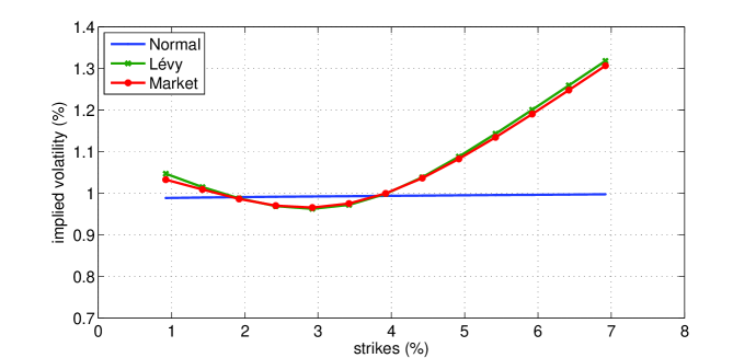
Figure 1. Implied normal volatilities for a 5Y option on the 3M LIBOR.

The results for a 5Y caplet on a composition of LIBOR rates are shown in Figure 2. It should not be surprising that the classical model does not produce any smile whereas the Lévy model does; note that the ATM prices are also different, where ATM $\approx 1.22$. Moreover, as has been observed in many other situations, the Brownian-driven model overprices the ATM options and underprices the in- and out-of-the-money options compared to the more realistic Lévy model.

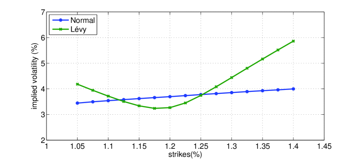
Figure 2. Implied normal volatilities for a 5Y option on composition.

5. Conclusion

We have presented valuation formulas, based on Fourier transforms, for pricing an option on the composition of LIBOR rates in the forward rate and forward price models driven by time-inhomogeneous Lévy processes. Analogous formulas can also be derived for the affine ‘forward price’-type framework proposed by KellerResselPapapantoleonTeichmann09; this framework combines the analytical tractability of the forward price framework described here with positive LIBOR rates.

The challenge ahead is to derive valuation formulas in the LIBOR model driven by a time-inhomogeneous Lévy process. This task requires some sophisticated approximations due to the structure of the dynamics in LIBOR market models; the interested reader is referred to SiopachaTeichmann07 SiopachaTeichmann07 and HubalekPapapantoleonSiopacha09 for a detailed analysis.

References

- [\citeauthoryearBjörk, Di Masi, Kabanov, and RunggaldierBjörk et al.1997] Björk, T., G. Di Masi, Y. Kabanov, and W. Runggaldier (1997). Towards a general theory of bond markets. Finance Stoch. 1, 141–174.
- [\citeauthoryearBlackBlack1976] Black, F. (1976). The pricing of commodity contracts. J. Financ. Econ. 3, 167–179.
- [\citeauthoryearBrace, Ga̧tarek, and MusielaBrace et al.1997] Brace, A., D. Ga̧tarek, and M. Musiela (1997). The market model of interest rate dynamics. Math. Finance 7, 127–155.
- [\citeauthoryearEberlein, Glau, and PapapantoleonEberlein et al.2008] Eberlein, E., K. Glau, and A. Papapantoleon (2008). Analysis of valuation formulae and applications to exotic options in Lévy models. Preprint, TU Vienna (arXiv/0809.3405).
- [\citeauthoryearEberlein, Jacod, and RaibleEberlein et al.2005] Eberlein, E., J. Jacod, and S. Raible (2005). Lévy term structure models: no-arbitrage and completeness. Finance Stoch. 9, 67–88.
- [\citeauthoryearEberlein and KlugeEberlein and Kluge2006a] Eberlein, E. and W. Kluge (2006a). Exact pricing formulae for caps and swaptions in a Lévy term structure model. J. Comput. Finance 9(2), 99–125.
- [\citeauthoryearEberlein and KlugeEberlein and Kluge2006b] Eberlein, E. and W. Kluge (2006b). Valuation of floating range notes in Lévy term structure models. Math. Finance 16, 237–254.
- [\citeauthoryearEberlein and KlugeEberlein and Kluge2007] Eberlein, E. and W. Kluge (2007). Calibration of Lévy term structure models. In M. Fu, R. A. Jarrow, J.-Y. Yen, and R. J. Elliott (Eds.), Advances in Mathematical Finance: In Honor of Dilip B. Madan, pp. 155–180. Birkhäuser.
- [\citeauthoryearEberlein and ÖzkanEberlein and Özkan2005] Eberlein, E. and F. Özkan (2005). The Lévy LIBOR model. Finance Stoch. 9, 327–348.
- [\citeauthoryearEberlein and RaibleEberlein and Raible1999] Eberlein, E. and S. Raible (1999). Term structure models driven by general Lévy processes. Math. Finance 9, 31–53.
- [\citeauthoryearHagan, Kumar, Lesniewski, and WoodwardHagan et al.2002] Hagan, P. S., D. Kumar, A. S. Lesniewski, and D. E. Woodward (2002). Managing smile risk. Wilmott magazine 18(11), 84–108.
- [\citeauthoryearHeath, Jarrow, and MortonHeath et al.1992] Heath, D., R. Jarrow, and A. Morton (1992). Bond pricing and the term structure of interest rates: a new methodology for contingent claims valuation. Econometrica 60, 77–105.
- [\citeauthoryearHenrardHenrard2005] Henrard, M. (2005). Swaptions: 1 price, 10 deltas, and … 6 1/2 gammas. Working paper.
- [\citeauthoryearHubalek, Papapantoleon, and SiopachaHubalek et al.2009] Hubalek, F., A. Papapantoleon, and M. Siopacha (2009). Taylor approximation of stochastic differential equations and application to the Lévy LIBOR model. Preprint, TU Vienna.
- [\citeauthoryearJacod and ShiryaevJacod and Shiryaev2003] Jacod, J. and A. N. Shiryaev (2003). Limit Theorems for Stochastic Processes (2nd ed.). Springer.
- [\citeauthoryearJamshidianJamshidian1997] Jamshidian, F. (1997). LIBOR and swap market models and measures. Finance Stoch. 1, 293–330.
- [\citeauthoryearKeller-Ressel, Papapantoleon, and TeichmannKeller-Ressel et al.2009] Keller-Ressel, M., A. Papapantoleon, and J. Teichmann (2009). A new approach to LIBOR modeling. Preprint, TU Vienna.
- [\citeauthoryearKlugeKluge2005] Kluge, W. (2005). Time-inhomogeneous Lévy processes in interest rate and credit risk models. Ph. D. thesis, University of Freiburg.
- [\citeauthoryearMiltersen, Sandmann, and SondermannMiltersen et al.1997] Miltersen, K. R., K. Sandmann, and D. Sondermann (1997). Closed form solutions for term structure derivatives with log-normal interest rates. J. Finance 52, 409–430.
- [\citeauthoryearPapapantoleonPapapantoleon2007] Papapantoleon, A. (2007). Applications of semimartingales and Lévy processes in finance: duality and valuation. Ph. D. thesis, University of Freiburg.
- [\citeauthoryearRaibleRaible2000] Raible, S. (2000). Lévy processes in finance: theory, numerics, and empirical facts. Ph. D. thesis, University of Freiburg.
- [\citeauthoryearSandmann, Sondermann, and MiltersenSandmann et al.1995] Sandmann, K., D. Sondermann, and K. R. Miltersen (1995). Closed form term structure derivatives in a Heath–Jarrow–Morton model with log-normal annually compounded interest rates. In Proceedings of the Seventh Annual European Futures Research Symposium Bonn, pp. 145–165. Chicago Board of Trade.
- [\citeauthoryearSiopacha and TeichmannSiopacha and Teichmann2007] Siopacha, M. and J. Teichmann (2007). Weak and strong Taylor methods for numerical solutions of stochastic differential equations. Preprint, TU Vienna. (arXiv/0704.0745).