Recoil-induced subradiance in a cold atomic gas

Abstract

Subradiance, i.e. the cooperative inhibition of spontaneous emission by destructive interatomic interference, can be realized in a cold atomic sample confined in a ring cavity and lightened by a two-frequency laser. The atoms, scattering the photons of the two laser fields into the cavity-mode, recoil and change their momentum. Under proper conditions the atomic initial momentum state and the first two momentum recoil states form a three-level degenerate cascade. A stationary subradiant state is obtained after that the scattered photons have left the cavity, leaving the atoms in a coherent superposition of the three collective momentum states. After a semiclassical description of the process, we calculate the quantum subradiant state and its Wigner function. Anti-bunching and quantum correlations between the three atomic modes of the subradiant state are demonstrated.

I Introduction

Recent experiments with Bose-Einstein Condensates (BEC) driven by a far off-resonant laser beam have demonstrated collective Superradiant Rayleigh MIT:1 ; MIT:2 ; Tokio ; LENS and Raman scattering Schneble ; Yoshi , sharing strong analogies with the superradiant emission from excited two-level atoms SR:review . In these experiments an elongated BEC scatters the pump photons into the end-fire modes along the major dimensions of the condensate, acquiring a momentum multiple of the two-photon recoil momentum $\hbar\vec{q}$, where $\vec{q}=\vec{k}-\vec{k}_{s}$ and $\vec{k}$ and $\vec{k}_{s}$ are the wave vectors of the pump and the scattered field. Theoretical works have shown that the Superradiant Rayleigh Scattering relies on the quantum collective atomic recoil (QCARL) gain mechanism, in which the fast escape of the emitted radiation from the active medium leads to the superradiant emission Gatelli ; JoB ; SR:CARL . The quantum regime of CARL CARL:1 ; CARL:2 occurs when the two-photon recoil frequency $\omega_{r}=\hbar q^{2}/2m$ is larger than the gain bandwidth, such that the recoil frequency shifts the atoms out of resonance inhibiting further scattering processes. As a consequence in the QCARL each atom coherently scatters a single pump photon, changing momentum by $\hbar q$. The process in which the atoms make a transition between two momentum states ($\vec{p}=0$ and $\vec{p}=\hbar\vec{q}$) has strong analogies with that of two-level atoms prepared in the excited state and decaying to the lower state by spontaneous and stimulated emission. However, the incoherent spontaneous emission dominating the two-level atomic decay is absent in the momentum transition, where spontaneous emission is associated to momentum diffusion due to the scattering force, which can be made very small if the laser is sufficiently detuned from the atomic resonance. The absence of Doppler broadening and the long decoherence time of a BEC allows to observe superradiance and coherent spontaneous emission much more easily than from electronic transitions in excited atoms, in which the decay is dominated by the incoherent spontaneous emission.

Another example of cooperative phenomena from excited two-level atoms is subradiance, i.e. the cooperative inhibition of spontaneous emission by a destructive interatomic interference. This phenomenon, whose existence has been proposed by Dicke (1954) in the same article predicting superradiance Dicke , has received less consideration than the more popular superradiance, also due to the difficulty of its experimental observation. In fact, the only experimental evidence has been done on 1985 by Pavolini et al. Pav . Among different schemes of multi-level systems in which subradiance was predicted, Crubellier et al., in a series of theoretical papers Cru1 ; Cru2 ; Cru3 ; Cru4 , proposed a three-level degenerate cascade configuration in which cooperative spontaneous emission is expected to exhibit new and striking subradiance effects.

In this paper we show that subradiance in a three-level degenerate cascade can be realized in a BEC inserted in a ring cavity and lightened by two laser fields with frequency difference twice the two-photon recoil frequency, as illustrated by fig.1.

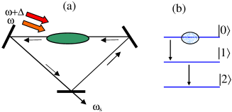
Figure 1: (a): Schematic diagram illustrating the geometry of a two-frequency pump CARL experiment; (b): three-level cascade scheme.

The frequency of the scattered photon is determined by energy and momentum conservation. The process consists in two steps. In the first step the atoms initially at rest scatter the laser photons of frequency $\omega$ into the cavity mode of frequency $\omega_{s}=\omega-\omega_{r}$, changing momentum from $0$ to $\vec{p}=\hbar\vec{q}$. In the second step the atom scatters the laser photon of frequency $\omega+\Delta$ changing their momentum from $\vec{p}=\hbar\vec{q}$ to ${\vec{p}}\,\,^{\prime}=2\hbar\vec{q}$. Since the change of the kinetic energy of the atom is $\Delta E=(p\,^{\prime}\,{}^{2}-p^{2})/2m=3\hbar\omega_{r}$, by energy conservation the frequency of the scattered photon is $\omega+\Delta-3\omega_{r}$ which coincides with the frequency generated in the first step when $\Delta=2\omega_{r}$. In this way a three-momentum-level degenerate cascade is realized in which the atoms, initially with momentum $\vec{p}=0$, change momentum to the intermediate value $\hbar\vec{q}$ and then to the final value $2\hbar\vec{q}$, emitting two degenerate photons of frequency $\omega_{s}=\omega-\omega_{r}$. In general the process, as described in ref.ASR , will continue with an other scattering of the photon of frequency $\omega+\Delta$ changing the atomic momentum from $2\hbar\vec{q}$ to $3\hbar\vec{q}$ with the emission of a photon of frequency $\omega+\Delta-5\omega_{r}=\omega-3\omega_{r}$ and so on. However, if the cavity linewidth is much narrower than the frequency difference, $\kappa\ll 2\omega_{r}$, these other frequencies will be damped out. Then, the oscillation of only the frequency $\omega_{s}=\omega-\omega_{r}$ in the cavity will restrict the momentum cascade to the three momentum states, $0$, $\hbar\vec{q}$ and $2\hbar\vec{q}$. A basic feature of this system is that the transition rates are proportional to the pump intensities, so that they can be varied with continuity. This makes the subradiance observation much easier than with a three-level cascade between electronic energy levels, where the transition rates are fixed by the branching ratios.

II Semiclassical treatment

II.1 General model

The quantum collective atomic recoil laser (QCARL) with a two-frequency pump is described by the following equations for the order parameter $\Psi(z,t)$ of the matter field and the cavity mode field amplitude $a(t)$ ASR :

$$i\noindent\frac{\partial\Psi}{\partial t} = -\frac{\hbar}{2m}\frac{\partial^{2}\Psi}{\partial z^{2}}+ig\left[\alpha(t)a^{*}e^{i(qz-\delta t)}-{\rm cc.}\right]\Psi$$ (1)

$$\noindent\frac{da}{dt} = gN\alpha(t)\int dz|\Psi|^{2}e^{i(qz-\delta t)}-\kappa a,$$ (2)

where $z$ is the coordinate along the cavity axis and $\alpha(t)=1+\epsilon\exp(-i\Delta t)$. These equations have been derived performing the adiabatic elimination of the atomic internal degrees of freedom Gatelli but replacing the pump field with $E_{p}=e^{i(\vec{k}\cdot\vec{x}-\omega t)}\left(E_{0}+E_{1}e^{-i\Delta t}\right)$. In Eqs.(1) and (2) $a(t)=(\epsilon_{0}V/2\hbar\omega_{s})^{1/2}E_{s}(t)$ is the dimensionless electric field amplitude of the scattered radiation beam with frequency $\omega_{s}$, $g=(\Omega_{0}/2\Delta_{0})(\omega d^{2}/2\hbar\epsilon_{0}V)^{1/2}$ is the coupling constant, $\Omega_{0}=dE_{0}/\hbar$ is the Rabi frequency of the pump laser incident with an angle $\phi$ with respect to the $z$ axis ($\phi=\pi$ if counterpropagating), with electric field $E_{0}$ and frequency $\omega$ detuned from the atomic resonance frequency $\omega_{0}$ by $\Delta_{0}=\omega-\omega_{0}$. The pump laser has a sideband with frequency $\omega+\Delta$, with $\Delta=2\omega_{r}$ [where $\omega_{r}=\hbar q^{2}/2m$ and $q=2k\sin(\phi/2)$], and electric field $E_{1}$ with $\epsilon=E_{1}/E_{0}$. The other parameters are: $d=\hat{\epsilon}\cdot\vec{d}$, the electric dipole moment of the atom along the polarization direction $\hat{\epsilon}$ of the laser, $V$, the cavity mode volume, $N$ the total number of atoms in the condensate, $\delta=\omega-\omega_{s}$, and $\kappa$, the cavity linewidth. The emitted frequency $\omega_{s}$ is within the cavity frequency linewidth, whereas the pump field is external to the cavity so that its frequencies are not dependent on the cavity ones. The order parameter $\Psi$ of the matter field is normalized such that $\int dz|\Psi|^{2}=1$.

If the condensate is much longer than the radiation wavelength and approximately homogeneous, then periodic boundary conditions can be applied on the atomic sample and the order parameter can be written as $\Psi(z,t)=\sum_{n}c_{n}(t)u_{n}(z)e^{-in\delta t}$, where $u_{n}(z)=(q/2\pi)^{1/2}\exp[in(qz)]$ are the momentum eigenstates with eigenvalues $p_{z}=n(\hbar q)$. Using this expansion, Eqs.(1) and (2) become:

$$\frac{dc_{m}}{dt} = -i\omega_{m}c_{m}+g[\alpha(t)a^{*}c_{m-1}-\alpha^{*}(t)ac_{m+1}]$$ (3)

$$\frac{da}{dt} = gN\alpha(t)\sum_{n}c_{m}c^{*}_{m+1}-\kappa a,$$ (4)

where $\omega_{n}=n(n\omega_{r}-\delta)$.

II.2 Three-level approximation

As as been discussed elsewhere Gatelli ; QCARL , if the gain rate is smaller than the recoil frequency the atoms recoil only along the positive direction of $\vec{q}$, absorbing a photon from the laser and emitting it into the cavity mode. Backward recoil, in which an atom absorbs a photon from the cavity mode and emits it into the laser mode, is inhibited by energy conservation. In this way, the laser photon of frequency $\omega$ induces a momentum transition from $m=0$ to $m=1$, emitting in the cavity a photon with frequency $\omega_{s}=\omega-\omega_{r}$; the laser photon of frequency $\omega+\Delta$ [with $\Delta=2\omega_{r}$] induces a momentum transition from $m=1$ and $m=2$, emitting an other photon of the same frequency $\omega_{s}$. If the cavity linewidth $\kappa$ is smaller less than $2\omega_{r}$, only the photons with frequency $\omega_{s}$ will survive in the cavity. Since further scattering would generate photons with frequencies $\omega-m\omega_{r}$, with $m=3,5,\dots$, which can not oscillate in the cavity, then the Hilbert space of the atoms is spanned by only the first three recoil momentum levels, $m=0,1,2$, and Eqs.(3) and (4) reduce to:

$$\frac{dc_{0}}{dt} = -g\alpha^{*}(t)ac_{1}$$ (5)

$$\frac{dc_{1}}{dt} = i(\delta-\omega_{r})c_{1}+g[\alpha(t)a^{*}c_{0}-\alpha^{*}(t)ac_{2}]$$ (6)

$$\frac{dc_{2}}{dt} = 2i(\delta-2\omega_{r})c_{2}+g\alpha(t)a^{*}c_{1}$$ (7)

$$\frac{da}{dt} = gN\alpha(t)(c_{0}c^{*}_{1}+c_{1}c^{*}_{2})-\kappa a.$$ (8)

Eqs.(5)-(8) contain fast oscillating terms. They can be eliminated introducing the slowly varying variable $\tilde{c}_{2}=c_{2}\exp(i\Delta t)$ and approximating Eqs.(5)-(8) neglecting the fast oscillating terms proportional to $\exp(\pm i\Delta t)$. In this way Eqs.(5)-(8) reduce to:

$$\frac{dc_{0}}{dt} = -gac_{1}$$ (9)

$$\frac{dc_{1}}{dt} = i(\delta-\omega_{r})c_{1}+g(a^{*}c_{0}-\epsilon a\tilde{c}_{2})$$ (10)

$$\frac{d\tilde{c}_{2}}{dt} = 2i(\delta-\omega_{r})\tilde{c}_{2}+g\epsilon a^{*}c_{1}$$ (11)

$$\frac{da}{dt} = gN(c_{0}c^{*}_{1}+\epsilon c_{1}\tilde{c}^{*}_{2})-\kappa a.$$ (12)

Eqs.(9)-(12) describe the three-level degenerate cascade of the atoms driven by two laser fields at frequencies $\omega$ and $\omega+2\omega_{r}$, respectively, and interacting with the self-generated cavity mode at the frequency $\omega_{s}=\omega-\omega_{r}$. Notice that the second transition rate, from $m=1$ to $m=2$, is proportional to the two pump amplitude ratio, $\epsilon$.

II.3 Subradiance in three-level degenerate cascade

Asymptotically, in a time much longer than $1/\kappa$, the photons leak the cavity and the total polarization in Eq.(12) vanishes:

$$c_{0}c^{*}_{1}+\epsilon c_{1}\tilde{c}^{*}_{2}=0.$$ (13)

On resonance ($\delta=\omega_{r}$) and with the atoms initially at rest ($c_{0}(0)=1$), the variables $c_{0}$, $c_{1}$, $c_{2}$ and $a$ are real and Eqs.(9)-(12) keep invariant the following quantity:

$$J=\epsilon^{2}c_{0}^{2}+\tilde{c}_{2}^{2}+2\epsilon c_{0}\tilde{c}_{2}=\epsilon^{2}.$$ (14)

From it we see that the atoms can not populate completely the final state $m=2$ (with $c_{2}=1$ and $c_{0}=0$) unless $\epsilon=1$. Hence, when $\epsilon\neq 1$ the atoms remain in the intermediate levels $m=0$ and $m=1$ in a subradiant state. Condition (13), together with the constraints (14) and the normalization $c_{0}^{2}+c_{1}^{2}+\tilde{c}_{2}^{2}=1$, determine univocally the steady-state solution reached asymptotically by the atoms. It is easy to show that for $\epsilon<1/\sqrt{3}$,

$$c_{0}=-\epsilon\tilde{c}_{2}=\frac{\epsilon^{2}}{1-\epsilon^{2}},\quad c_{1}=\left[1-\frac{\epsilon^{2}(1+\epsilon^{2})}{(1-\epsilon^{2})^{2}}\right]^{1/2}$$ (15)

whereas for $\epsilon>1/\sqrt{3}$,

$$c_{0}=\frac{1-\epsilon^{2}}{1+\epsilon^{2}},\quad c_{1}=0,\quad\tilde{c}_{2}=-\frac{2\epsilon}{1+\epsilon^{2}}$$ (16)

Fig.2 shows the steady-state populations $P_{i}=|c_{i}|^{2}$ for $i=0,1,2$ plotted vs. $\epsilon$. We observe that increasing $\epsilon$ from zero the population of the intermediate state, $P_{1}$, decreases and the population of the final state, $P_{2}$, increases. They are equal for $\epsilon=1/2$, with $c_{0}=1/3$ and $c_{1}=-c_{2}=2/3$. The population of the initial state $P_{0}$ increases too and reaches a local maximum for $\epsilon=1/\sqrt{3}$ with $c_{0}=1/2$, $c_{1}=0$ and $c_{2}=\sqrt{3}/2$. Then, for $\epsilon>1/\sqrt{3}$ the intermediate state $m=1$ is empty ($c_{1}=0$) and the population of the initial state $P_{0}$ decreases to zero for $1/\sqrt{3}<\epsilon<1$; then for $\epsilon>1$ it increases until it equals the population of the final state $P_{2}$ when $\epsilon=1+\sqrt{2}$. For $\epsilon>1+\sqrt{2}$ the population of the initial state, $P_{0}$, is larger than that of the final state, $P_{2}$. However, this case appears stationary only because the semiclassical model neglects spontaneous emission. The quantum treatment, reported in the next section, shows that the stationary subradiant state may exist only for $0<\epsilon<1+\sqrt{2}$.

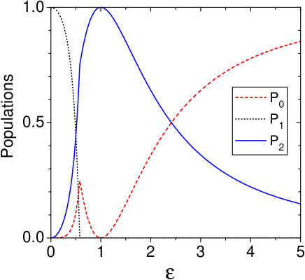
Figure 2: Semiclassical subradiance solution: populations of the three states, $P_{0}$ (dashed red line), $P_{1}$ (dotted gray line) and $P_{2}$ ( continuous blue line) as a function of $\epsilon$, as given by Eqs. (15) and (16).

In order to illustrate how the system evolves toward the subradiance state, fig.3 shows the time evolution of the field $|a|^{2}$ (fig.3a), and the three populations, (fig.3b) [$P_{0}$ (dashed blue line), $P_{1}$ (red continuous line) and $P_{2}$ (dashed-dotted black line)], obtained solving the complete equations (3) and (4) for $g\sqrt{N}=0.01\omega_{r}$, $\kappa=0.006\omega_{r}$, $\delta=\omega_{r}$ and $\epsilon=1/2$, with initial condition $c_{0}(0)=1$, $c_{i\neq 0}(0)=0$ and $a(0)=0.01$. The final populations are $P_{0}=1/9$ and $P_{1}=P_{2}=4/9$, according to Eq. (15).

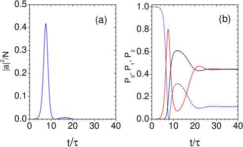
Figure 3: Time evolution of the radiated intensity $|a|^{2}$, (a), and the three populations $P_{0}$ (dashed blue line), $P_{1}$ (red continuous line) and $P_{2}$ (dashed-dotted black line) vs. $t/\tau$, where $\tau=(g\sqrt{N})^{-1}$, for $g\sqrt{N}=0.01\omega_{r}$, $\kappa=0.006\omega_{r}$, $\delta=\omega_{r}$ and $\epsilon=1/2$.

In order to test the dependence of the subradiance state on the frequency difference $\Delta$ between the two pump fields, figure 4 shows the asymptotic coherence $C_{1,2}=|c_{1}c_{2}^{*}|$ between the intermediate and the final states vs. $\Delta$ for $g=0.01\omega_{r}$, $\delta=\omega_{r}$, $\epsilon=1/2$, $\kappa=0.003\omega_{r}$ (dashed blue line), $\kappa=0.006\omega_{r}$ (dashed-dot red line) and $\kappa=0.012\omega_{r}$ (continuous black line). The result shows that subradiance requires a very fine tuning of the pump frequency difference near $2\omega_{r}$, within a precision $\delta\omega\ll g\sqrt{N}$.

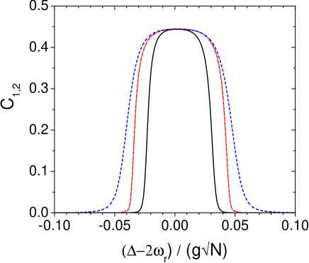
Figure 4: Asymptotic coherence $C_{1,2}=|c_{1}c_{2}^{*}|$ between the intermediate and the final states vs. $(\Delta-2\omega_{r})/g\sqrt{N}$ for $g=0.01\omega_{r}$, $\delta=\omega_{r}$, $\epsilon=1/2$, $\kappa=0.003\omega_{r}$ (dashed blue line), $\kappa=0.006\omega_{r}$ (dashed-dot red line) and $\kappa=0.012\omega_{r}$ (continuous black line).

As a second example, figs. 5 and 6 show that same case as in figs.3 and 4 but with $\epsilon=1+\sqrt{2}$. In this case $P_{1}=0$ and $P_{0}=P_{2}=1/2$. We note that whereas in the case $\epsilon=1/2$ the resonance linewidth of fig.4 decreases when the cavity losses $\kappa$ increases, on the contrary in the case $\epsilon=1+\sqrt{2}$ the linewidth increases with $\kappa$ and it is about a factor $100$ larger. Hence the subradiance with $\epsilon=1/2$ is more sensible to the frequency mismatch than that with $\epsilon=1+\sqrt{2}$.

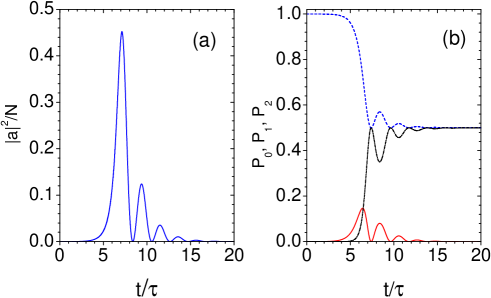
Figure 5: Time evolution of the radiated intensity $|a|^{2}$ (a) and the three populations $P_{0}$ (dashed blue line), $P_{1}$ (red continuous line) and $P_{2}$ (dashed-dotted black line) as a function of $t/\tau$, where $\tau=(g\sqrt{N})^{-1}$, for the same parameters of fig.3 and $\epsilon=1+\sqrt{2}$.

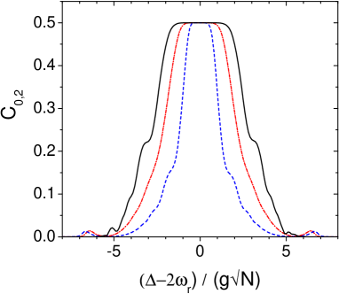
Figure 6: Asymptotic coherence $C_{0,2}=|c_{0}c_{2}^{*}|$ between the initial and the final states vs. $(\Delta-2\omega_{r})/g\sqrt{N}$ for $g=0.01\omega_{r}$, $\delta=\omega_{r}$, $\epsilon=1+\sqrt{2}$, $\kappa=0.003\omega_{r}$ (dashed blue line), $\kappa=0.006\omega_{r}$ (dashed-dot red line) and $\kappa=0.012\omega_{r}$ (continuous black line).

III quantum treatment

III.1 The subradiant state

Let now obtain the subradiant state quantum-mechanically, treating the amplitude $c_{n}$ as bosonic operators $\hat{c}_{n}$ with commutation rules $[\hat{c}_{m},\hat{c}_{n}^{\dagger}]=\delta_{m,n}$. Then, according to Eq.(13) the subradiant state $|sr\rangle$ satisfies:

$$(\hat{c}_{0}\hat{c}_{1}^{\dagger}+\epsilon\hat{c}_{1}\hat{c}_{2}^{\dagger})|sr\rangle=0$$ (17)

(we omit the tilde on $\hat{c}_{2}$). It is possible to demonstrate (see Appendix A) that for a system of $N$ atoms (with $N$ even) there are $N/2$ subradiant states $|sr\rangle_{p}$, with $p=1,2,\dots,N/2$, defined as

$$|sr\rangle_{p} = C_{p}\sum_{k=0}^{p}\frac{(-1/2\epsilon)^{k}}{k!}\sqrt{\frac{(2k)!(N-p-k)!}{(p-k)!}}$$ (18)

$$\times|p-k,2k,N-p-k\rangle,$$

where $|m,n,l\rangle=|m\rangle_{0}|n\rangle_{1}|l\rangle_{2}$ and $C_{p}$ is a normalization constant. The index $p$ is related to the population difference between the initial and final states, since $N_{0}-N_{2}=2p-N$. The case $p=0$ corresponds to the state $|0,0,N\rangle$. The link between the subradiant state $|sr\rangle_{p}$ and the semiclassical solution (15) and (16) is provided by the correspondence between $p$ and the population difference $N_{0}-N_{2}=N(c_{0}^{2}-c_{2}^{2})$ in the limit $N\gg 1$. For $\epsilon<1/\sqrt{3}$, $p=(N/2)(1-2\epsilon^{2})/(1-\epsilon^{2})$ and for $\epsilon>1/\sqrt{3}$, $p=N[1-4\epsilon^{2}/(1+\epsilon^{2})^{2}]$. As particular cases, $p=N/3$ for $\epsilon=1/2$ and $p=N/4$ for $\epsilon=1/\sqrt{3}$. Furthermore, $p=0$ for $\epsilon=1$ and $p=N/2$ for $\epsilon=1+\sqrt{2}$. Hence $1+\sqrt{2}$ is the maximum value of $\epsilon$, giving the following subradiant state:

$$|sr\rangle_{N/2} = C_{N/2}\sum_{k=0}^{N/2}\frac{(-1/2\epsilon)^{k}}{k!}\sqrt{(2k)!}$$ (19)

$$\times\left|\frac{N}{2}-k,2k,\frac{N}{2}-k\right\rangle.$$

For large $N$, the average value of $k$ is $\langle k\rangle=1/4\epsilon=(\sqrt{2}-1)/4$, with variance $\sigma_{k}^{2}=\langle k\rangle$.

From the state (18) and the correspondence between $p$ and $\epsilon$ we may evaluate the average populations $P_{i}=\langle N_{i}\rangle/N$, with $i=0,1,2$, as a function of $\epsilon$. The result is compared in fig.7 with the semiclassical solution (15) and (16), for $N=32$. We observe that the quantum solution has not a sharp transition at $\epsilon=1/\sqrt{3}$ as the classical one, but there a tail which becomes negligible for $N\gg 1$.

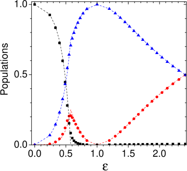
Figure 7: Quantum subradiance solution: population fraction of the three states, $P_{0}$ (red circles), $P_{1}$ (black squares) and $P_{2}$ (blue triangles) vs. $\epsilon$, obtained from Eq. (18) with $N=32$. The dashed lines show for comparison the semiclassical solution of fig.2.

III.2 Wigner function

Here we show the Wigner function of the subradiance state $|sr\rangle$ in order to get some more properties of the system. We start from the definition

$$W(\alpha_{0},\alpha_{1},\alpha_{2})=\int\prod_{i=0}^{2}\frac{d^{2}\xi_{i}}{\pi^{2}}\;e^{\xi_{i}^{*}\alpha_{i}-\alpha_{i}^{*}\xi_{i}}\chi(\xi_{0},\xi_{1},\xi_{2})\>,$$ (20)

where $\alpha_{i}$ and $\xi_{i}$ are complex numbers and $\chi$ is the characteristic function defined as

$$\chi(\xi_{0},\xi_{1},\xi_{2}) = \langle sr|\hat{D}_{0}(\xi_{0})\hat{D}_{1}(\xi_{1})\hat{D}_{2}(\xi_{2})|sr\rangle,$$ (21)

where $\hat{D}_{j}(\xi_{j})=\exp(\xi_{j}\hat{c}^{\dagger}_{j}-\xi^{*}_{j}\hat{c}_{j})$ is a displacement operator for the $j$-th mode. A straightforward calculation, reported in the Appendix B, yields

$$\chi(\xi_{0},\xi_{1},\xi_{2})=e^{-(|\xi_{0}|^{2}+|\xi_{1}|^{2}+|\xi_{2}|^{2})/2}\times$$

$$\sum_{k=0}^{p}\beta_{k}\;L_{p-k}(|\xi_{0}|^{2})\;L_{2k}(|\xi_{1}|^{2})\;L_{N-p-k}(|\xi_{2}|^{2}),$$ (22)

and

$$W(\alpha_{0},\alpha_{1},\alpha_{2})=\left(\frac{2}{\pi}\right)^{3}e^{-2(|\alpha_{0}|^{2}+|\alpha_{1}|^{2}+|\alpha_{2}|^{2})}\times$$

$$\sum_{k=0}^{p}\beta_{k}\;L_{p-k}(4|\alpha_{0}|^{2})\;L_{2k}(4|\alpha_{1}|^{2})\;L_{N-p-k}(4|\alpha_{2}|^{2}),$$ (23)

where

$$\beta_{k}=C_{p}^{2}\;\frac{(2k)!(N-p-k)!}{(p-k)!(k!)^{2}}\left(\frac{1}{2\epsilon}\right)^{2k}$$ (24)

and $L_{n}(x)$ is the Laguerre polynomial. Notice that the Wigner function depends only on the modulus of $\alpha_{i}$ and not from its phase. As expected, in general it is negative due to the presence of the Laguerre polynomials. By integrating over the other two mode variables, from Eq.(23) we obtain the single-mode Wigner functions:

$$W(\alpha_{0}) = \frac{2}{\pi}e^{-2|\alpha_{0}|^{2}}\sum_{k=0}^{p}(-1)^{p-k}\beta_{k}\;L_{p-k}(4|\alpha_{0}|^{2})$$ (25)

$$W(\alpha_{1}) = \frac{2}{\pi}e^{-2|\alpha_{1}|^{2}}\sum_{k=0}^{p}\beta_{k}\;L_{2k}(4|\alpha_{1}|^{2})$$ (26)

$$W(\alpha_{2}) = \frac{2}{\pi}e^{-2|\alpha_{2}|^{2}}\sum_{k=0}^{p}(-1)^{N-p-k}\beta_{k}\;$$ (27)

$$\times L_{N-p-k}(4|\alpha_{2}|^{2}).$$

In order to investigate the characteristics of the subradiance state, let’s consider some specific example. An interesting case is when $\epsilon=1/2$ and $p=N/3$, for which the semiclassical theory yields $P_{1}=P_{2}=4/9$. Fig.8(a) shows the probability $\beta_{k}$ vs. $k$ for $N=36$ and $p=12$. The probability is maximum for $k=8$, the average value is $\langle k\rangle=7.14$ and the standard deviation is $\sigma_{k}=2.64$. The single-mode Wigner functions $W_{i}=W(\alpha_{i})$ are shown in fig.8(b-d): $W_{0}$ has a maximum at $|\alpha_{0}|=2$ and $W_{1}$ and $W_{2}$ have a maximum at $|\alpha_{1}|=|\alpha_{2}|=4$, in agreement with the population values predicted by the semiclassical solution. However, $W_{1}$ differs considerably from $W_{2}$ with a strong oscillation near $|\alpha_{1}|=0$, probably due to the tail of the distribution at small $k$ observed in fig.8(a). The single-mode Wigner functions present a pronounced maximum around which they are positive, plus an oscillating quantum background.

As a second example we consider the case $\epsilon=1+\sqrt{2}$, for which the semiclassical theory yields $P_{1}=0$ and $P_{0}=P_{2}=1/2$. In the quantum model it corresponds to the maximally anti-symmetric state (19) with $p=N/2$. Fig.9(a) shows the probability $\beta_{k}$ vs. $k$ for $N=36$ and $p=18$. The probability is maximum for $k=0$ and decreases rapidly to zero for larger $k$, with $\langle k\rangle=0.1$ and $\sigma_{k}=0.35$. The single-mode Wigner functions $W_{i}$ are shown in fig.9(b-d). $W_{0}$ and $W_{2}$ are equal and very similar to the Wigner function of the number state $|N/2\rangle$, $W(\alpha)=(4/\pi)\exp(-2|\alpha|^{2})L_{N/2}(4|\alpha|^{2})$ Walls . Furthermore, $W_{1}$ is equal to the vacuum Wigner function $W(\alpha)=(4/\pi)\exp(-2|\alpha|^{2})$. In this case $N/2$ pairs of atoms with momentum $0$ and $2\hbar q$ are produced.

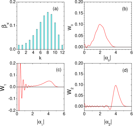
Figure 8: Subradiant state for $N=36$, $p=12$ and $\epsilon=1/2$: (a) probability $\beta_{k}$ vs. $k$; (b) $W_{0}$ vs. $|\alpha_{0}|$; (c) $W_{1}$ vs. $|\alpha_{1}|$; (d) $W_{2}$ vs. $|\alpha_{2}|$.

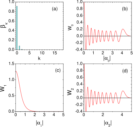
Figure 9: Subradiant state for $N=36$, $p=18$ and $\epsilon=1+\sqrt{2}$: (a) probability $\beta_{k}$ vs. $k$; (b) $W_{0}$ vs. $|\alpha_{0}|$; (c) $W_{1}$ vs. $|\alpha_{1}|$; (d) $W_{2}$ vs. $|\alpha_{2}|$.

The three-mode Wigner function (23), after integrating one mode variable, yields the following two-mode Wigner functions:

$$W(\alpha_{0},\alpha_{1}) = \left(\frac{2}{\pi}\right)^{2}e^{-2(|\alpha_{0}|^{2}+|\alpha_{1}|^{2})}\sum_{k=0}^{p}(-1)^{p+k}\beta_{k}L_{p-k}(4|\alpha_{0}|^{2})L_{2k}(4|\alpha_{1}|^{2})$$ (28)

$$W(\alpha_{0},\alpha_{2}) = \left(\frac{2}{\pi}\right)^{2}e^{-2(|\alpha_{0}|^{2}+|\alpha_{2}|^{2})}\sum_{k=0}^{p}\beta_{k}L_{p-k}(4|\alpha_{0}|^{2})L_{N-p-k}(4|\alpha_{2}|^{2})$$ (29)

$$W(\alpha_{1},\alpha_{2}) = \left(\frac{2}{\pi}\right)^{2}e^{-2(|\alpha_{1}|^{2}+|\alpha_{2}|^{2})}\sum_{k=0}^{p}(-1)^{p-k}\beta_{k}L_{p-k}(4|\alpha_{1}|^{2})L_{2k}(4|\alpha_{2}|^{2})$$ (30)

Figures 10, 11 and 12 (color online) show the two-mode Wigner functions $W_{i,j}=W(\alpha_{i},\alpha_{j})$ as a function of $|\alpha_{i}|$ and $|\alpha_{j}|$, for $i,j=0,1,2$ for the case $N=36$ and $p=12$, corresponding to $\epsilon=1/2$ (see fig.8): The red color corresponds to a negative value of the functions. We observe several zones of negativity indicating non classical correlations between the two modes. In particular, $W_{0,1}$ and $W_{1,2}$ show strong correlations of the modes $0$ and $2$ with the mode $1$, which has strong oscillations, whereas $W_{0,2}$ is larger near the vacuum value $(0,0)$. Hence, we can say that qualitatively the modes $0$ and $2$ behave quasi-classically whereas the mode $1$ has feature similar to a number state. Figures 13, shows $W_{0,2}$ vs. $|\alpha_{0}|$ and $|\alpha_{2}|$ for the case $N=36$ and $p=18$, corresponding to $\epsilon=1+\sqrt{2}$ (see fig.9). The two-mode Wigner function looks the product of two single-mode number Wigner functions shown in fig.9(b) and (d), with a bi-dimensional regular mesh of positive and negative zones.

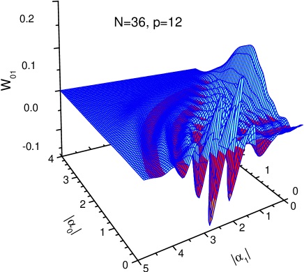
Figure 10: Two-mode Wigner function $W(\alpha_{0},\alpha_{1})$ for $N=36$, $p=12$.

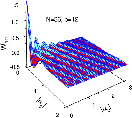
Figure 11: Two-mode Wigner function $W(\alpha_{0},\alpha_{2})$ for $N=36$, $p=12$.

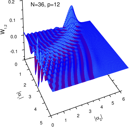
Figure 12: Two-mode Wigner function $W(\alpha_{1},\alpha_{2})$ for $N=36$, $p=12$.

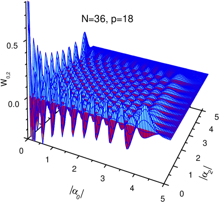
Figure 13: Two-mode Wigner function $W(\alpha_{0},\alpha_{2})$ for $N=36$, $p=18$.

III.3 Atom statistics

We calculate now the equal-time intensity correlation and cross-correlation functions, defined respectively as:

$$g_{i}^{(2)}(0) = \frac{\langle\hat{c}_{i}^{{\dagger}}\hat{c}_{i}^{{\dagger}}\hat{c}_{i}\hat{c}_{i}\rangle}{\langle\hat{N}_{i}\rangle^{2}}$$ (31)

$$g_{i,j}^{(2)}(0) = \frac{\langle\hat{N}_{i}\hat{N}_{j}\rangle}{\langle\hat{N}_{i}\rangle\langle\hat{N}_{j}\rangle},$$ (32)

with $i=0,1,2$, $i\neq j$ and $\hat{N}_{i}=\hat{c}_{i}^{{\dagger}}\hat{c}_{i}$. For a classical field there is an upper limit to the second-order equal-time cross correlation function given by the Cauchy-Schwartz inequality

$$g_{i,j}^{(2)}(0)\leq[g_{i}^{(2)}(0)\;g_{j}^{(2)}(0)]^{1/2}.$$ (33)

Quantum-mechanical fields, however, can violate this inequality and are instead constrained by

$$g_{i,j}^{(2)}(0)\leq\left[g_{i}^{(2)}(0)+\frac{1}{\langle\hat{N}_{i}\rangle}\right]^{1/2}\left[g_{j}^{(2)}(0)+\frac{1}{\langle\hat{N}_{j}\rangle}\right]^{1/2}$$ (34)

which reduces to the classical results in the limit of large occupation numbers. We obtain the following expressions for the subradiant state:

$$g_{0}^{(2)}(0) = 1+\frac{\sigma_{k}^{2}-\langle\hat{N}_{0}\rangle}{\langle\hat{N}_{0}\rangle^{2}}$$ (35)

$$g_{1}^{(2)}(0) = 1+\frac{4\sigma_{k}^{2}-\langle\hat{N}_{1}\rangle}{\langle\hat{N}_{1}\rangle^{2}}$$ (36)

$$g_{2}^{(2)}(0) = 1+\frac{\sigma_{k}^{2}-\langle\hat{N}_{2}\rangle}{\langle\hat{N}_{2}\rangle^{2}}$$ (37)

where $\sigma_{k}^{2}=\langle k^{2}\rangle-\langle k\rangle^{2}$ and

$$\langle k^{m}\rangle=\sum_{k=0}^{p}k^{m}\beta_{k}.$$

The cross-correlation functions are

$$g_{0,1}^{(2)}(0) = 1-\frac{2\sigma_{k}^{2}}{\langle\hat{N}_{0}\rangle\langle\hat{N}_{1}\rangle}$$ (38)

$$g_{0,2}^{(2)}(0) = 1+\frac{\sigma_{k}^{2}}{\langle\hat{N}_{0}\rangle\langle\hat{N}_{2}\rangle}$$ (39)

$$g_{1,2}^{(2)}(0) = 1-\frac{2\sigma_{k}^{2}}{\langle\hat{N}_{1}\rangle\langle\hat{N}_{2}\rangle}.$$ (40)

From (35)-(40) it follows that

$$g_{0,1}^{(2)}(0)^{2} = \left(g_{0}^{(0)}(0)+\frac{1}{\langle\hat{N}_{0}\rangle}\right)\left(g_{1}^{(2)}(0)+\frac{1}{\langle\hat{N}_{1}\rangle}\right)-\sigma^{2}\left(\frac{1}{\langle\hat{N}_{0}\rangle}+\frac{2}{\langle\hat{N}_{1}\rangle}\right)^{2}$$ (41)

$$g_{0,2}^{(2)}(0)^{2} = \left(g_{0}^{(0)}(0)+\frac{1}{\langle\hat{N}_{0}\rangle}\right)\left(g_{2}^{(2)}(0)+\frac{1}{\langle\hat{N}_{2}\rangle}\right)-\sigma^{2}\left(\frac{1}{\langle\hat{N}_{0}\rangle}-\frac{1}{\langle\hat{N}_{2}\rangle}\right)^{2}$$ (42)

$$g_{1,2}^{(2)}(0)^{2} = \left(g_{1}^{(2)}(0)+\frac{1}{\langle\hat{N}_{1}\rangle}\right)\left(g_{2}^{(2)}(0)+\frac{1}{\langle\hat{N}_{2}\rangle}\right)-\sigma^{2}\left(\frac{2}{\langle\hat{N}_{1}\rangle}+\frac{1}{\langle\hat{N}_{2}\rangle}\right)$$ (43)

showing that $g_{ij}^{(2)}(0)$ are consistent with the quantum inequality (34). Fig.14 shows the intensity correlation functions $g_{i}^{(2)}(0)$ for $i=0,1,2$, for the subradiance state (18). We obtain that $g_{2}^{(2)}(0)$ (continuous red line) is less than unity for all the values of $\epsilon$ and $g_{0}^{(2)}(0)$ (dotted blue line) is less than unity for $\epsilon>0.56$. So anti-bunching occurs for the momentum states $m=0$ and $m=2$, but not for the state $m=1$.

Fig.15-17 show the eventual violation of the Cauchy-Schwartz inequality (33) for $g_{i,j}^{(2)}$ (continuous line). The dashed line is the classical upper limit $[g_{i}^{(2)}(0)g_{j}^{(2)}(0)]^{1/2}$ and the dotted line is the quantum upper limit $[(g_{i}^{(2)}(0)+1/\langle\hat{N}_{i}\rangle)(g_{j}^{(2)}(0)+1/\langle\hat{N}_{j}\rangle)]^{1/2}$. We found that $g_{0,1}^{(2)}$ is always consistent with the classical inequality, whereas $g_{0,2}^{(2)}$ and $g_{1,2}^{(2)}$ violate the Cauchy-Schwartz inequality (33) for all the $\epsilon$ and for $\epsilon<0.47$, respectively, showing the existence of quantum correlations between the modes $m=0$ and $m=2$ and between the modes $m=1$ and $m=2$. For $\epsilon>1/\sqrt{3}$, $g_{0,2}^{(2)}$ is close to the upper limit of the quantum inequality (34).

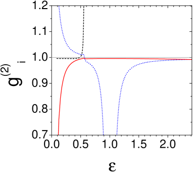
Figure 14: Intensity correlation functions vs. $\epsilon$: $g_{0}^{(2)}(0)$ (dotted blue line), $g_{1}^{(2)}(0)$ (dashed black line) and $g_{2}^{(2)}(0)$ (continuous red line).

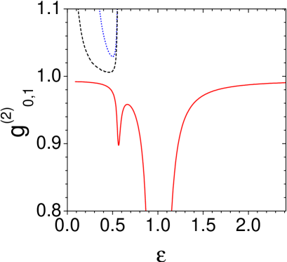
Figure 15: Cross correlation function $g_{0,1}^{(2)}(0)$ (continuous red line) vs. $\epsilon$. The dashed black line indicates the classical upper limit of the inequality (33); the dotted blue line indicates the quantum upper limit of the inequality (34).

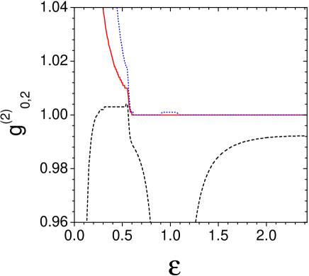
Figure 16: Same as in fig.15 but for $g_{0,2}^{(2)}(0)$.

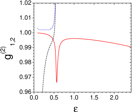
Figure 17: Same as in fig.15 but for $g_{1,2}^{(2)}(0)$.

IV conclusions

We have investigated a possible way to observe subradiance in a Bose-Einstein condensate in a high-finesse ring cavity, scattering photons from a two-frequency pump laser into a single-frequency cavity mode via the quantum collective atomic recoil lasing (QCARL) mechanism. Subradiance occurs in a degenerate cascade between three motional levels separated by the two-photon momentum recoil $\hbar\vec{q}$, where $\vec{q}=\vec{k}-\vec{k}_{s}$ is the momentum transfer between pump and cavity mode. The observation of subradiance in momentum transitions of cold atomic samples presents several advantages and differences with respect to the electronic transitions of excited two-level atoms. First, the momentum transitions are not affected by the spontaneous emission if the pump laser is sufficiently detuned from the atomic resonance. Second, the atomic condensates have a long life and a very long coherence time, allowing the preparation and the further manipulation of the subradiant state. Third, the subradiance is realized among collective motional states containing a large number of atoms. Subradiance as well superradiance do not need that the dimension of the sample is smaller than the radiation wavelength, as in superradiance by excited atoms. For these reasons, subradiance between motional states of ultracold atoms may be important for the study of the decoherence-free subspaces sought in quantum information dfss . Other recent proposals of realizing subradiance in matter wave require a very fine control of single atoms in optical cavities foldi , which can be very problematic experimentally. On the other hand, the experimental activity on Superradiant Rayleigh scattering and CARL with Bose-Einstein condensates MIT:1 ; Tub:PRL has achieved important progresses and a subradiance experiment with BEC in a ring cavity could be feasible with the present day techniques. At ultracold temperature and with a coupling constant $g\sqrt{N}$ much less than the recoil frequency $\omega_{r}$ should be possible, using two laser fields with frequency difference $2\omega_{r}$, to restrict the momentum transition to only the first two recoil momentum states. Recent experiments on superradiant scattering from a BEC pumped by a two-frequency laser beam TFP:1 ; TFP:2 have shown that the momentum transitions are enhanced by the presence of the second pump detuned by $2\omega_{r}$. However, only inserting the BEC in a high-finesse ring cavity it will possible to limit the transition sequence to only two. Then, varying the relative intensity of the two pump laser beams should be possible to probe the transition from superradiance to subradiance. As an example of possible parameters, subradiance could be observed in a ring cavity similar to that realized in Tübingen Tub:PRA (with length $L=87$mm, beam waist $w=100\,\mu m$ and finesse $F=5\times 10^{5}$, about 5 times the presently achieved value) with $\kappa=0.2\omega_{r}$ and $g\sqrt{N}=0.2\omega_{r}$. This last value can be obtained using a ⁸⁷Rb condensate (with $\omega_{r}=(2\pi)15$kHz) with $N=10^{4}$ atoms at a temperature of some tens of nK, driven by two laser beams with $P_{0}=174$mW, $\Delta_{0}=-(2\pi)3$THz and a frequency difference precision of $\delta\omega\leq 5$kHz. Subradiance will be reached in about $100\mu$s, less than the decoherence time of the BEC.

Appendix A The subradiance state

In order to demonstrate Eq.(18) let’s consider a state of the form

$$|sr\rangle=\sum_{n_{1}=0}^{N}\sum_{(n_{0},n_{2})}f(n_{0},n_{2})|n_{0},n_{1},n_{2}\rangle$$

where the second sum is over all the pairs $(n_{0},n_{2})$ such that $n_{0}+n_{2}=N-n_{1}$. When substituted in (17), it yields

$$\sum_{n_{1}=0}^{N-1}\sum_{\begin{array}[]{c}{{}_{(n_{0},n_{2})}}_{,}{{}_{n_{0}\neq 0}}\\ _{n_{0}+n_{2}=N-n_{1}}\end{array}}f(n_{0},n_{2})\sqrt{n_{0}(n_{1}+1)}|n_{0}-1,n_{1}+1,n_{2}\rangle$$ (46)

$$+ \epsilon\sum_{n_{1}=1}^{N}\sum_{\begin{array}[]{c}{{}_{(n_{0},n_{2})}}_{,}{{}_{n_{2}\neq N}}\\ _{n_{0}+n_{2}=N-n_{1}}\end{array}}f(n_{0},n_{2})\sqrt{n_{1}(n_{2}+1)}|n_{0},n_{1}-1,n_{2}+1\rangle=0.$$ (49)

After having redefined the indexes $n_{1}$ and $n_{2}$ in the sums, it becomes

$$\left\{\sum_{n_{1}=1}^{N}\sum_{\begin{array}[]{c}{{}_{(n_{0},n_{2})}}\\ {{}_{n_{0}\neq N}}\end{array}}f(n_{0}+1,n_{2})\sqrt{(n_{0}+1)n_{1}}+\epsilon\sum_{n_{1}=0}^{N-1}\sum_{\begin{array}[]{c}{{}_{(n_{0},n_{2})}}\\ {{}_{n_{2}\neq 0}}\end{array}}f(n_{0},n_{2}-1)\sqrt{(n_{1}+1)n_{2}}\right\}|n_{0},n_{1},n_{2}\rangle=0.$$ (50)

The terms in the curl bracket of Eq. (50) vanish when the following conditions are met:

1. In the second sum on $n_{1}$ in the curl bracket the term with $n_{1}=N$ is missing: since in the first sum $n_{0}=n_{2}=0$ when $n_{1}=N$, it yields $f(1,0)=0$.

2. In the first sum on $n_{1}$ in the curl bracket the term with $n_{1}=0$ is missing: then the second sum on $n_{1}$ with $n_{1}=0$, $n_{2}=N-n_{0}$ and $n_{2}\neq 0$ yields

   $$f(n_{0},N-n_{0}-1)=0\quad,\quad n_{0}=0\dots,N-1.$$ (51)

3. The remaining sum in (50) yields:

   $$\sum_{\begin{array}[]{c}{{}_{(n_{0},n_{2})}}\\ {}_{n_{0}+n_{2}=N-n_{1}}\end{array}}f(n_{0}+1,n_{2})\sqrt{(n_{0}+1)n_{1}}+\epsilon\sum_{\begin{array}[]{c}{{}_{(n_{0},n_{2})}}_{,}{{}_{n_{2}\neq 0}}\\ {}_{n_{0}+n_{2}=N-n_{1}}\end{array}}f(n_{0},n_{2}-1)\sqrt{(n_{1}+1)n_{2}}=0,$$ (52)

   with $n_{1}=1,\dots,N-1$. In the second sum of Eq.(50) the term $n_{2}=0$ is missing, so in the first sum the term with $n_{2}=0$ and $n_{0}=N-n_{1}$ vanishes and yields $f(k,0)=0$ with $k=2,\dots,N$. Together with the result of item 1, it yields

   $$f(k,0)=0\quad,\qquad k=1,2,\dots,N$$ (53)

   whereas the remaining terms of Eq.(52) yield

   $$\sqrt{(n_{0}+1)n_{1}}f(n_{0}+1,N-n_{0}-n_{1})=-\epsilon\sqrt{(n_{1}+1)(N-n_{0}-n_{1})}f(n_{0},N-n_{0}-n_{1}-1)$$ (54)

   with $n_{1}=1,\dots,N-1$ and $n_{0}=0,\dots,N-n_{1}$.

For $n_{1}=2$ Eq.(54) yields

$$\sqrt{2(n_{0}+1)}f(n_{0}+1,N-n_{0}-2)=-\epsilon\sqrt{3(N-n_{0}-3)}f(n_{0},N-n_{0}-3)\quad,\quad n_{0}=0,\dots,N-3$$ (55)

Since from Eq.(51) $f(n_{0}+1,N-n_{0}-2)=0$, then

$$f(n_{0},N-n_{0}-3)=0\quad,\quad n_{0}=0\dots,N-3.$$ (56)

Continuing with all the even values of $n_{1}$, it is easy to show that

$$f(n_{0},N-n_{0}-k)=0\quad,\quad k=1,3,\dots,N-n_{0}\,(odd),\quad n_{0}=0\dots,N-k.$$ (57)

Hence, the only terms different from zero are those with $n_{1}=2q+1$ and $q=0,\dots,N/2-1$, yielding:

$$f(n_{0}+1,N-n_{0}-2q-1)=-\epsilon\sqrt{\frac{(2q+2)(N-n_{0}-2q-1)}{(n_{0}+1)(2q+1)}}f(n_{0},N-n_{0}-2q-2),$$ (58)

where $n_{0}=0,\dots,N-(2q+1)$. Eq.(58) provides a recurrence relation for the index $n_{0}$ with a given $n_{0}+q$. In fact the difference between the first and second index of $f(a,b)$ in both the left and right terms of Eq.(58) is $\Delta=b-a=N-2(n_{0}+q+1)$. So, introducing the new index $p=n_{0}+q+1$, Eq.(58) can be written, for $p=1,\dots,N/2$, as:

$$f(p-q-1,N-p-q-1)=-\frac{1}{\epsilon}\sqrt{\frac{(2q+1)(p-q)}{(2q+2)(N-p-q)}}f(p-q,N-p-q)\quad,\quad q=0,\dots,p$$ (59)

By iteration of Eq.(59) we obtain

$$f(p-q,N-p-q)=\left(-\frac{1}{\epsilon}\right)^{q}\sqrt{\frac{(2q+1)!!}{(2q)!!}\frac{p!(N-p-q)!}{(p-q)!(N-p)!}}f(p,N-p)\quad,\quad q=0,\dots,p$$ (60)

where $(2k)!!=2k\cdot(2k-2)\dots 2\cdot 1$ and $(2k+1)!!=(2k+1)\cdot(2k-1)\dots 3\cdot 1$. Since $(2q+1)!!/(2q)!!=(2q)!/(2^{q}q!)^{2}$, finally we obtain :

$$|sr\rangle=C_{p}\sum_{q=0}^{p}\left(-\frac{1}{2\epsilon}\right)^{q}\sqrt{\frac{(2q)!(N-p-q)!}{(q!)^{2}(p-q)!}}|p-q,2q,N-p-q\rangle$$ (61)

where $C_{p}=[p!/(N-p)!]^{1/2}f(p,N-p)$.

Appendix B Derivation of the subradiant Wigner function

We demonstrate Eq.(22). Writing the displacement operator as a product of operators, $\hat{D}(\xi)=\exp(-|\xi|^{2}/2)\exp(\xi\hat{c}^{\dagger})\exp(-\xi^{*}\hat{c})$ and using the formula

$$\exp(-\xi^{*}\hat{c})|k\rangle=\sum_{n=0}^{k}\frac{(-\xi^{*})^{n}}{n!}\sqrt{\frac{k!}{(k-n)!}}|k-n\rangle$$

we obtain

$$\langle k^{\prime}|\hat{D}(\xi)|k\rangle=e^{-|\xi|^{2}/2}L_{k}(|\xi|^{2})\delta_{k,k^{\prime}}$$ (62)

where

$$L_{k}(x)=\sum_{n=0}^{k}(-1)^{n}\begin{pmatrix}k\\ n\\ \end{pmatrix}\frac{x^{n}}{n!}$$

is the Laguerre Polynomial of order $k$. Using (62) in (21) with the subradiant state (18) we obtain

$$\chi(\xi_{0},\xi_{1},\xi_{2})=e^{-(|\xi_{0}|^{2}+|\xi_{1}|^{2}+|\xi_{2}|^{2})/2}\times$$

$$\sum_{k=0}^{p}\beta_{k}\;L_{p-k}(|\xi_{0}|^{2})\;L_{2k}(|\xi_{1}|^{2})\;L_{N-p-k}(|\xi_{2}|^{2}).$$ (63)

In order to evaluate the Wigner function (20) we must calculate an integral of the form:

$$I_{m}(\alpha)=\int d^{2}\xi\;e^{\xi^{*}\alpha-\alpha^{*}\xi-|\xi|^{2}/2}L_{m}(|\xi|^{2}).$$ (64)

Introducing polar coordinates $\xi=-ir\exp(i\phi)$ and $\alpha=|\alpha|\exp(i\psi)$ it transforms into

$$I_{m}(\alpha)=\int_{0}^{\infty}dr\;re^{-r^{2}/2}L_{m}(r^{2})\int_{0}^{2\pi}d\phi e^{2ir|\alpha|\cos(\phi-\psi)}=$$

$$2\pi\int_{0}^{\infty}dr\;re^{-r^{2}/2}L_{m}(r^{2})J_{0}(2r|\alpha|)$$ (65)

Where $J_{0}(x)$ is the Bessel function of zero order. Using the formula Grad :

$$\int_{0}^{\infty}dx\;xe^{-ax^{2}/2}L_{n}(bx^{2}/2)J_{0}(xy)=$$

$$\frac{(a-b)^{n}}{a^{n+1}}e^{-y^{2}/2a}L_{n}\left(\frac{by^{2}}{2a(b-a)}\right)$$ (66)

we obtain

$$I_{m}(\alpha)=2\pi(-1)^{m}e^{-2|\alpha|^{2}}L_{m}(4|\alpha|^{2})$$ (67)

So, from the definition of Wigner function (20) and using Eqs. (63) and (67) we obtain

$$W(\alpha_{0},\alpha_{1},\alpha_{2})=\frac{1}{\pi^{6}}\sum_{k=0}^{p}\beta_{k}\;I_{p-k}(\alpha_{0})I_{2k}(\alpha_{1})I_{N-p-k}(\alpha_{2})$$ (68)

which coincides with Eq.(23). Using the formula Grad

$$\int_{0}^{\infty}dx\;e^{-x/a}L_{m}(x)=a(1-a)^{n}$$ (69)

we have

$$\frac{1}{\pi^{2}}\int d^{2}\alpha\;I_{m}(\alpha)=1.$$ (70)

From (67), (68) and (70) we obtain the expressions (25)-(27) and (28)-(30) of the one-mode and two-mode reduced Wigner functions, respectively.

References

- (1) S. Inouye, A.P. Chikkatur, D.M. Stamper-Kurn, J. Stenger, D.E. Pritchard and W. Ketterle, Science 285, 571 (1999).
- (2) S. Inouye, T. Pfau, S. Gupta, A.P. Chikkatur, A. Görlitz, D.E. Pritchard and W. Ketterle, Nature 402, 641 (1999).
- (3) M. Kozuma, Y. Suzuki, Y. Torii, T. Sugiura, T. Kugam, E.W. Hagley, L. Deng, Science 286, 2309 (1999).
- (4) L. Fallani, C. Fort, N. Piovella, M.M. Cola, F.S. Cataliotti, M. Inguscio, and R. Bonifacio, Phys. Rev. A 71, 033612 (2005).
- (5) D. Schneble et al.,Phys. Rev. A 69, 041601(R) (2004).
- (6) Y. Yoshikawa et al., Rev. A 69, 041603(R) (2004).
- (7) M. Gross and S. Haroche, Phys. Rep. 93, 301 (1982).
- (8) N. Piovella, M. Gatelli and R. Bonifacio, Optics Comm. 194, 167 (2001).
- (9) G.R.M. Robb, N. Piovella, and R. Bonifacio, J. Opt. B: Quantum Semiclass. Opt. 7 93 (2005).
- (10) N. Piovella, M. Gatelli, L. Martinucci, R. Bonifacio, B.W.J. McNeil, and G.R.M. Robb, Laser Physics, 12, 188 (2002).
- (11) R. Bonifacio and L. De Salvo Souza, Nucl. Instrum. and Meth. in Phys. Res. A 341, 360 (1994).
- (12) R. Bonifacio, L. De Salvo, L.M. Narducci and E.J. D’Angelo, Phys. Rev. A 50, 1716 (1994).
- (13) R.H. Dicke, Phys. Rev. 93, 99 (1954).
- (14) D. Pavolini, A. Crubellier, P. Pillet, L. Cabaret, and S. Liberman, Phys. Rev. Lett. 54, 1917 (1985).
- (15) A. Crubellier, S. Liberman, D. Pavolini, and P. Pillet, J. Phys. B: At. Mol. Phys. 18, 3811 (1985).
- (16) A. Crubellier, and D. Pavolini, J. Phys. B: At. Mol. Phys. 19, 2109 (1986).
- (17) A. Crubellier, J. Phys. B: At. Mol. Phys. 20, 971 (1987).
- (18) A. Crubellier, and D. Pavolini, J. Phys. B: At. Mol. Phys. 20, 1451 (1987).
- (19) M.M. Cola, L. Volpe, and N. Piovella, Phys. Rev. A 79, 013613 (2009).
- (20) N. Piovella, M. M. Cola and R. Bonifacio, Phys. Rev. A 67, 013817 (2003).
- (21) D.F.Walls, and G.J. Milburn, Quantum Optics, (Springer, Berlin, 1994) p. 64.
- (22) D.A. Lidar, I.L. Chuang, and K.B. Whaley, Phys. Rev. Lett. 81, 2594 (1998).
- (23) P. Földi, M.G. Benedict, and A. Czirják, Phys. Rev. A 65, 021802(R) (2002).
- (24) S. Slama, S. Bux, G. Krenz, C. Zimmermann, and Ph.W. Courteille, Phys. Rev. Lett. 98, 053603 (2007).
- (25) N. Bar-Gill, E.E. Rowen, and N. Davidson, Phys. Rev. A 76, 043603 (2007).
- (26) F. Yang, X. Zhou, J. Li, Y. Chen, L. Xia, and X. Chen, Phys. Rev. A 78, 043611 (2008).
- (27) S. Slama, G. Krenz, S. Bux, C. Zimmermann, Ph.W. Courteille, Phys. Rev. A 75, 063620 (2007).
- (28) I.S. Gradshteyn and I.M. Ryzhuk, Table of Intagrals, Series and Products, (Academic Press, San Diego, 2000), p. 803-805.