Heat transport and phonon localization in mass-disordered harmonic crystals

Abstract

We investigate the steady state heat current in two and three dimensional disordered harmonic crystals in a slab geometry, connected at the boundaries to stochastic white noise heat baths at different temperatures. The disorder causes short wavelength phonon modes to be localized so the heat current in this system is carried by the extended phonon modes which can be either diffusive or ballistic. Using ideas both from localization theory and from kinetic theory we estimate the contribution of various modes to the heat current and from this we obtain the asymptotic system size dependence of the current. These estimates are compared with results obtained from a numerical evaluation of an exact formula for the current, given in terms of a frequency transmission function, as well as from direct nonequilibrium simulations. These yield a strong dependence of the heat flux on boundary conditions. Our analytical arguments show that for realistic boundary conditions the conductivity is finite in three dimensions but we are not able to verify this numerically, except in the case where the system is subjected to an external pinning potential. This case is closely related to the problem of localization of electrons in a random potential and here we numerically verify that the pinned three dimensional system satisfies Fourier’s law while the two dimensional system is a heat insulator. We also investigate the inverse participation ratio of different normal modes.

I Introduction

Energy transport in dielectric crystals at low temperatures is limited by isotope mass disorder and by anharmonicities. For a crystal coupled to thermal heat baths, in a slab geometry, the total energy transported may in addition depend on how the bath is coupled to the boundaries of the bulk. In this paper we will ignore anharmonicities but study the two other effects in considerable depth.

Based on empirical evidence, one generically expects the validity of Fourier’s law, i.e. , for a slab in contact with heat reservoirs at different temperatures the average energy current, $J$, should be proportional to $1/N$, with $N$ being the slab length. There have been many attempts to derive Fourier’s law from microscopic dynamics. Using very reasonable physical assumptions of local equilibrium and the notion of the mean free path traveled by phonons between collisions yields a heuristic derivation of Fourier’s law. There is however no fully convincing derivation. There have also been many computer simulations of the heat flux in the nonequilibrium stationary states of anharmonic crystals kept in contact with thermal reservoirs at different temperatures, and theoretical analysis based on the Green-Kubo formalism dharrev09 ; LLP03 ; BLR00 . These studies suggest (but there is no proof despite some claims) that Fourier’ law is not valid for one and two dimensional systems, even in the presence of anharmonic interactions, unless the system is also subjected to an external substrate pinning potential. Generically it is found that, for a system in contact with heat reservoirs at different fixed temperatures, the heat current density $J$ scales anomalously with system length $N$ as

$$J\sim\frac{1}{N^{\mu}}~{},$$ (1)

with $\mu\neq 1$. The effective thermal conductivity behaves then as $\kappa\sim N^{\alpha}$ where $\alpha=1-\mu$. For two dimensional systems there are some analytic studies which suggest $\kappa\sim\ln(N)$. Recent experiments on heat conduction in nanotubes and graphene flakes have reported observations which indicate such divergence of $\kappa$ with system size chang08 ; nika09 .

For heat conduction in the ordered harmonic crystal there are exact results from which one has $\mu=0$ in all dimensions rieder67 ; nakazawa70 . Heat conduction in a disordered harmonic crystal will be affected by Anderson localization anderson58 and by phonon scattering.

In this paper we report results of heat conduction studies in $2D$ and $3D$ disordered harmonic lattices with scalar displacements, connected to heat baths modeled by Langevin equations with white noise. We pay particular attention to the interplay between localization effects, boundary effects, and the role of long wavelength modes. The steady state heat current is given exactly as an integral over all frequencies of a phonon transmission coefficient. Using this formula and heuristic arguments, based on localization theory and kinetic theory results, we estimate the system size dependence of the current. The main idea behind our arguments is that the phonon states can be classified as ballistic modes, diffusive modes and localized modes. The classification refers both to the character of the eigenfunctions as well as to their transmission properties. Ballistic modes are spatially extended and approximately periodic; their transmission is independent of system size. Diffusive modes are extended but non-periodic and their transmission decays as $1/N$. For localized modes transmission decays exponentially with $N$. In the context of kinetic theory calculations, the ballistic modes are the low frequency modes with phonon mean free path $\ell_{K}(\omega)\stackrel{{\scriptstyle>}}{{\sim}}N$, and their contribution to the current leads to divergence of the thermal conductivity. Here we will carefully examine the effect of boundary conditions on these modes.

Numerically we use two different approaches to study the nonequilibrium stationary state. The first is a numerical one which relies on the result that the current can be expressed in terms of a transmission coefficient. This transmission coefficient can be written in terms of phonon Green’s functions and we implement efficient numerical schemes to evaluate this. The second approach is through direct nonequilibrium simulations of the Langevin equations of motion and finding the steady state current and temperature profiles. We have also studied properties of the isolated system, i.e., of the disordered lattice without coupling to heat baths and looked at the normal mode frequency spectrum and the wavefunctions. One measure of the degree of localization of the normal modes of the isolated system is the so-called inverse participation ratio [IPR, defined in Eq. (10) below]. We have carried out studies of the IPR and linked these with the results from the transmission study.

Phonon localization: This is closely related to the electron localization problem. The effect of localization on linear waves in disordered media has been most extensively studied in the context of the Schrödinger equation for non-interacting electrons moving in a disordered potential. Looking at the eigenstates and eigenfunctions of the isolated system of a single electron in a disordered potential one finds that, in contrast to the spatially extended Bloch states in periodic potentials, there are now many eigenfunctions which are exponentially localized in space. It was argued by Mott and Twose mott61 and by Borland borland63 , and proven rigorously by Goldsheid et al. goldsheid77 , that in one dimension ($1D$) all states are exponentially localized. In two dimensions ($2D$) there is no proof but it is believed that again all states are localized. In three dimensions ($3D$) there is expected to be a transition from extended to localized states as the energy is moved towards the band edges lee85 . The transition from extended to localized states, which occurs when the disorder is increased, changes the system from a conductor to an insulator. The connection between localization and heat transport in a crystal is complicated by the fact that phonons of all frequencies can contribute to energy transmission across the system. In particular account has to be taken of the fact that low frequency phonon modes are only weakly affected by disorder and always remain extended. The heat current carried by a mode which is localized on a length scale $\ell$, decays with system length $N$ as $e^{-N/\ell}$. This $\ell$ depends on the phonon frequency and low frequency modes for which $\ell\sim N$ will therefore be carriers of the heat current. The net current then depends on the nature of these low frequency modes and their scattering due to boundary conditions (BCs).

A renormalization group study of phonon localization in a continuum vector displacement model was carried out by John et al.  john83 . They found that much of the predictions of the scaling theory of localization for electrons carry over to the phonon case. Specifically they showed that in one and two dimensions all non-zero frequency phonons are localized with the low frequency localization length diverging as $\ell\sim\omega^{-2}$ and $\sim e^{c/\omega^{2}}$, respectively (where $c>0$ is some constant). This means that in $1D$ all modes with $\omega\stackrel{{\scriptstyle>}}{{\sim}}\omega_{c}^{L}=N^{-1/2}$ are localized while in $2D$ all modes with $\omega\stackrel{{\scriptstyle>}}{{\sim}}\omega_{c}^{L}=[\log(N)]^{-1/2}$ are localized. In $3D$ the prediction is that there is an $\omega_{c}^{L}$ independent of $N$ above which all modes are localized. However this study does not make any statements on the system size dependence of the conductivity.

Kinetic theory: If one considers the low frequency extended phonons, then the effect of disorder is weak and in dimensions $d>1$ one expects that localization effects can be neglected and kinetic theory should be able to provide an accurate description. In this case one can think of Rayleigh scattering of phonons. This gives an effective mean free path $\ell_{K}(\omega)\sim\omega^{-(d+1)}$ [see appendix A] , for dimensions $d>1$, and a diffusion constant $D(\omega)=v\ell_{K}(\omega)$ where $v$, the sound velocity, can be taken to be a constant. For a finite system of linear dimension $N$ we have $D(\omega)=vN$ for $\omega\stackrel{{\scriptstyle<}}{{\sim}}N^{-1/(d+1)}$. Kinetic theory then predicts

$$\kappa=\int_{N^{-1}}^{\omega_{\rm max}}d\omega\rho(\omega)D(\omega)~{},$$ (2)

where $\rho(\omega)\sim\omega^{d-1}$ is the density of states and we get $\kappa\sim N^{1/(d+1)}$ implying $\mu=d/(d+1)$. The divergence of the phonon mean free path at low frequencies and the resulting divergence of the thermal conductivity of a disordered harmonic crystal has been discussed in the literature and it has been argued that anharmonicity is necessary to make $\kappa$ finite callaway59 ; ziman72 .

Simulation results: There have been only few simulation studies of heat conduction in three dimensional disordered systems and none have been definitive concerning the validity of Fourier’s law shimada00 ; shiba08 . In two dimension a diverging thermal conductivity was reported in lee05 . Some other studies have also looked at heat conduction in glassy systems at low temperatures where the harmonic approximation was used allen89 ; xu09 but these did not address the questions of $N$-dependence of $\kappa$ and the validity of Fourier’s law.

In $1D$ it is well known from rigorous results and numerical studies that $\alpha\neq 0$ and its value is strongly dependent on boundary conditions matsuda70 ; rubin71 ; casher71 ; oconnor74 ; dhar01 ; roydhar08 . For fixed BCs one has $\alpha=-1/2$ while for free BCs, $\alpha=1/2$. The precise definitions of the different BCs will be given later. Here we explain the different physical situations they correspond to. If we model the heat reservoirs themselves by infinite ordered harmonic crystals then Langevin type equations for the system dharroy06 are obtained on eliminating the bath degrees of freedom. The two different BCs then emerge naturally. Fixed BCs correspond to reservoirs with properties different from the system (e.g. different spring constants) and in this case one finds that effectively the particles at the boundaries (those coupled to reservoirs) experience an additional harmonic pinning potential. Free BCs correspond to the case where the reservoir is simply an extension of the system (without disorder) and in this case the end particles are unpinned. Free BCs have been studied in the literature in the context of heat conduction in one dimensional chains rubin71 and in studies on nanotubes savic08 ; stoltz08 . In this paper we study lattices with both fixed and free BCs although we think that fixed BCs are more realistic.

In the presence of an external pinning potential low frequency modes are suppressed, hence one expects qualitative differences in transport properties. The pinned system has often been used as a model system to study the validity of Fourier’s law. It has no translational invaraince and is thus more closely related to the problem of electrons moving in a random potential. Here we consider systems with and without external pinning potentials.

The rest of the paper is organized as follows. In Sec. (II) we define the specific model studied by us and present some general results for heat conduction in harmonic Hamiltonian systems connected to Langevin baths. We also give some details of the numerical and simulation methods used in the paper. The transfer matrix approach used in evaluating the phonon transmission function is explained in Appendix B. In Sec. (III) a brief review of results for the one dimensional case and the heuristic arguments for the higher dimensional cases are given. In Sec. (IV) we present results from both the numerical approach and from nonequilibrium simulations. The main results presented are for transmission functions, IPRs of normal modes and the system size dependence of the current in two and three dimensional disordered harmonic lattices. Along the way we also present results for the density of states $\rho(\omega)$. Finally we conclude with a discussion in Sec. (V).

II Models and methods

For simplicity we consider only the case where longitudinal and transverse vibration modes are decoupled and hence we can describe the displacement at each site by a scalar variable. Also we restrict our study to $d$-dimensional hypercubic lattices. Let us denote the lattice points by the vector ${\bf{n}}=\{n_{1},n_{2},...,n_{d}\}$ with $n_{\nu}=1,2,...,N$. The displacement of a particle at the lattice site ${\bf{n}}$ is given by $x_{\bf{n}}$. In the harmonic approximation the system Hamiltonian is given by

$$H = \sum_{{\bf{n}}}\frac{1}{2}{m_{\bf{n}}\dot{x}_{{\bf{n}}}^{2}}+\sum_{{\bf{n}},\hat{{\bf{e}}}}\frac{k}{2}(x_{{\bf{n}}}-x_{{\bf{n}}+\hat{{\bf{e}}}})^{2}+\frac{k_{o}}{2}\sum_{\bf{n}}{x_{{\bf{n}}}^{2}}~{},$$ (3)

where $\hat{{\bf{e}}}$ refers to the $2d$ nearest neighbors of any site and we impose boundary conditions which will be specified later. We have also included an external pinning harmonic potential with spring constant $k_{o}$, which we will sometimes set equal to zero. We consider a binary mass disordered crystal. Specifically we set the masses of exactly half the particles at randomly chosen sites to be $\bar{m}-\Delta$ and the rest to be $\bar{m}+\Delta$. Thus $\Delta$ gives a measure of the disorder.

We couple all the particles at $n_{1}=1$ and $n_{1}=N$ to heat reservoirs, at temperatures $T_{L}$ and $T_{R}$ respectively, and use periodic boundary conditions in the other $(d-1)$ directions. The heat conduction takes place along the $1$ direction. Each layer with constant $n_{1}$ consists of $N^{\prime}=N^{d-1}$ particles. The heat baths are modeled by white noise Langevin equations of motion for the particles coupled to the baths. Using the notation ${\bf{n}}=(n_{1},{\bf{n}}^{\prime})$, the equations of motion are given by:

$${m}_{{\bf{n}}}\ddot{x}_{{\bf{n}}}=-\sum_{\hat{{\bf{e}}}}k(x_{\bf{n}}-x_{{\bf{n}}+\hat{{\bf{e}}}})-k_{o}x_{{\bf{n}}}+\delta_{n_{1},1}(-\gamma\dot{x}_{{\bf{n}}}$$

$$~{}~{}~{}~{}~{}~{}~{}~{}~{}+\eta^{L}_{{\bf{n}}^{\prime}}-k^{\prime}x_{{\bf{n}}})+\delta_{n_{1},N}(-\gamma\dot{x}_{{\bf{n}}}+\eta^{R}_{{\bf{n}}^{\prime}}-k^{\prime}x_{{\bf{n}}})~{},~{}~{}~{}~{}~{}$$ (4)

where the dissipative and noise terms are related by the usual fluctuation dissipation relations

$$\langle\eta^{L}_{{\bf{n}}^{\prime}}(t)\eta^{L}_{{\bf{l}}^{\prime}}(t^{\prime})\rangle = 2\gamma k_{B}T_{L}\delta(t-t^{\prime})\delta_{{\bf{n}}^{\prime}{\bf{l}}^{\prime}}~{},~{}~{}~{}$$

$$\langle\eta^{R}_{{\bf{n}}^{\prime}}(t)\eta^{R}_{{\bf{l}}^{\prime}}(t^{\prime})\rangle = 2\gamma k_{B}T_{R}\delta(t-t^{\prime})\delta_{{\bf{n}}^{\prime}{\bf{l}}^{\prime}}~{}.$$ (5)

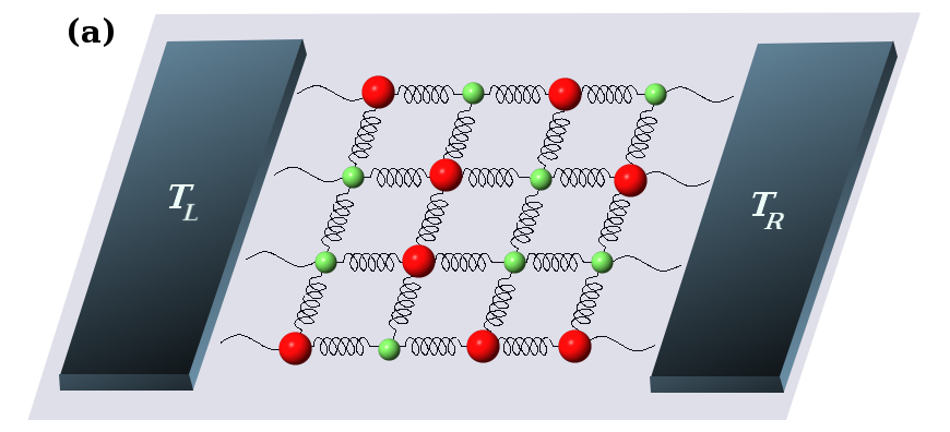
(a) Free boundaries

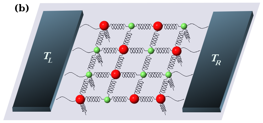
(b) Fixed boundaries

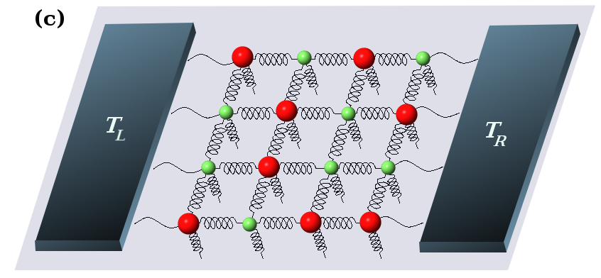
(c) Pinned lattice

Figure 1: A schematic diagram of a two-dimensional mass-disordered lattice of particles connected by harmonic springs and connected to heat baths at temperatures $T_{L}$ and $T_{R}$. Red and green colours indicate particles of different masses. Pinning refers to the presence of a spring attaching a particle to the substrate. In (a) there is no pinning, in (b) boundary particles are pinned and in (c) all sites are pinned.

The particles at the surfaces $n_{1}=1,N$ experience additional harmonic pinning potentials with spring constants $k^{\prime}$ arising from coupling to the heat reservoirs. We consider two kinds of boundary conditions at the surfaces connected to reservoirs: (i) fixed BCs $k^{\prime}>0$ and (ii) free BCs $k^{\prime}=0$. As discussed in the introduction fixed BCs correspond to reservoirs with properties different from the system while free reservoirs correspond to the case where the reservoir is really an extension of the system but without disorder. For the pinned case we only consider fixed BC. A schematic of the models and the different boundary conditions that we have studied is given in Fig. (1).

Henceforth we will use dimensionless variables: force-constants are measured in units of $k$, masses in units of the average mass $\bar{m}$, time in units of the inverse frequency $\Omega^{-1}=(\bar{m}/k)^{1/2}$, displacements are in units of the lattice spacing $a$, friction constant $\gamma$ is in units of $\bar{m}\Omega$, and finally temperature is measured in units of $\bar{m}a^{2}\Omega^{2}/k_{B}$.

Driven by the reservoirs at two different temperatures $T_{L}$ and $T_{R}$ the system reaches a nonequilibrium steady state. Our main interest will be in the steady state heat current in the system. Given the Langevin equations of motion Eq (4), one can find a formal general expression for the current. Let us denote by ${X}$ a column vector with $N^{d}$ elements consisting of the displacements at all lattice sites. Similarly let ${\dot{X}}$ represent the vector for velocities at all sites. Then we can write the Hamiltonian in Eq. (3) in the compact form $H=\frac{1}{2}{\dot{X}}^{T}\mathcal{M}{\dot{X}}+\frac{1}{2}{X}^{T}\mathcal{V}{X}~{}$, which defines the diagonal mass matrix $\mathcal{M}$ and the force constant matrix $\mathcal{V}$. With this notation we have the following form for the steady state current per bond from the left to the right reservoir dharroy06 ; casher71 :

$$\mathcal{J} = \frac{\Delta T}{4\pi N^{\prime}}\int_{-\infty}^{\infty}d\omega{\mathcal{T}}_{N}(\omega)~{},$$ (6)

where

$${\mathcal{T}}_{N}(\omega) = 4~{}Tr[\mathcal{I}_{L}(\omega)\mathcal{G}^{+}(\omega)\mathcal{I}_{R}(\omega)\mathcal{G}^{-}(\omega)]~{},$$ (7)

$$\mathcal{G}^{+}(\omega) = [-\omega^{2}\mathcal{M}+\mathcal{V}-\mathcal{S}^{+}_{L}-\mathcal{S}^{+}_{R}]^{-1}~{},~{}~{}\mathcal{G}^{-}=[\mathcal{G}^{+}]^{*}$$

and $\Delta T=T_{L}-T_{R}$. The ${\mathcal{S}}^{+}_{L}$, ${\mathcal{S}}^{+}_{R}$ represent terms arising from the coupling to the left and right baths respectively, and ${\mathcal{I}}_{L,R}=Im[{\mathcal{S}}^{+}_{L,R}]$. The specific form of $\mathcal{S}^{+}_{L,R}$ for our system described by Eqs. (4) is given in Appendix B. The matrix $\mathcal{G}^{+}(\omega)$ can be identified as the phonon Green’s function of the system with self-energy corrections due to the baths dharroy06 . The integrand in Eq. (6) $\mathcal{T}_{N}(\omega)$ can be thought of as the transmission coefficient of phonons at frequency $\omega$ from the left to the right reservoir. It will vanish, when $N\to\infty$ , at values of $\omega$ for which the disorder averaged density of states is zero. Note that due to the harmonic nature of the forces the dependence of the heat flux on the reservoir temperatures enters only through the term $\Delta T$ in Eq. (6). The above expression for the current is of the Landauer form and has been derived using various other approaches such as scattering theory rego98 ; blencowe99 and the nonequilibrium Green’s function formalism yamamoto06 ; wang06 .

Numerical approach: In Appendix B we describe how ${\mathcal{T}}_{N}$ can be expressed in a form amenable to accurate numerical computation. The system sizes we study are sufficiently large so that $\mathcal{T}_{N}(\omega)$ has appreciable values only within the range of frequencies of normal modes of the isolated system, i.e., corresponding to $\gamma=0$ in Eq. (4). Outside this range we find that the transmission rapidly goes to zero. By performing a discrete sum over the transmitting range of frequencies we do the integration in Eq. (6) to obtain the heat current density $\mathcal{J}$. In evaluating the discrete sum over $\omega$, step sizes of $\delta\omega=0.01-0.0001$ are used and we verified convergence in most cases. With our choice of units we have $k=1,\bar{m}=1$ and we fixed $\Delta T=1$. Different values of the mass variance $\Delta$ and the on-site spring constant $k_{o}$ were studied for two and three dimensional lattices of different sizes. It is expected that the value of the exponent $\mu$ will not depend on $\gamma$ and in our calculations we mostly set $\gamma=1$, except when otherwise specified.

Simulation approach: The simulations of Eq. (4) are performed using a velocity-Verlet scheme as given in allen . The current and temperature profiles in the system are obtained from the following time averages in the nonequilibrium steady state:

$$\mathcal{J}_{1} = \frac{1}{N^{\prime}}\sum_{{\bf{n}}^{\prime}}\frac{\gamma}{m_{(1,{\bf{n}}^{\prime})}}\left[T_{L}-m_{(1,{\bf{n}}^{\prime})}\langle\dot{x}^{2}_{(1,{\bf{n}}^{\prime})}\rangle\right],$$

$$\mathcal{J}_{n} = -\frac{1}{N^{\prime}}\sum_{{\bf{n}}^{\prime}}~{}\langle~{}[x_{(n,{\bf{n}}^{\prime})}-x_{(n-1,{\bf{n}}^{\prime})}]~{}\dot{x}_{(n,{\bf{n}}^{\prime})}~{}\rangle~{},$$

$$~{}~{}~{}~{}~{}~{}~{}~{}~{}~{}~{}~{}~{}~{}~{}~{}~{}~{}~{}~{}~{}~{}~{}~{}~{}n=2,3,...,N~{},$$

$$\mathcal{J}_{N+1} = -\frac{1}{N^{\prime}}\sum_{{\bf{n}}^{\prime}}\frac{\gamma}{m_{(N,{\bf{n}}^{\prime})}}\left[T_{R}-m_{(N,{\bf{n}}^{\prime})}\langle\dot{x}^{2}_{(N,{\bf{n}}^{\prime})}\rangle\right]~{},$$

$$T_{n} = \frac{1}{N^{\prime}}\sum_{{\bf{n}}^{\prime}}m_{(n,{\bf{n}}^{\prime})}\langle~{}\dot{x}^{2}_{(n,{\bf{n}}^{\prime})}~{}\rangle~{},~{}~{}~{}n=1,2,...,N~{}.$$

We then obtained the average current $\mathcal{J}=(\sum_{n=1}^{N+1}\mathcal{J}_{N})/(N+1)$. In the steady state one has $\mathcal{J}_{n}=\mathcal{J}$ for all $n$ and stationarity can be tested by checking how accurately this is satisfied. We chose a step size of $\Delta t=0.005$ and equilibrated the system for over $10^{8}$ time steps. Current and temperature profiles were obtained by averaging over another $10^{8}$ time steps. The parameters $T_{L}=2.0,T_{R}=1.0$ are kept fixed and different values of the mass variance $\Delta$ and the on-site spring constant $k_{o}$ are simulated.

The value of $\mathcal{T}_{N}(\omega)$, $\mathcal{J}$ and $T_{n}$ depend, of course, on the particular disorder realization. Mostly we will here be interested in disorder averages of these quantities which we will denote by $[\mathcal{T}],J=[\mathcal{J}]$ and $[T_{n}]$. We also define the disorder averaged transmission per bond with the notation

$$T(\omega)=\frac{1}{N^{\prime}}[\mathcal{T}(\omega)]~{}.$$

Numerical analysis of eigenmodes and eigenfunctions:  We have studied the properties of the normal modes of the disordered harmonic lattices in the absence of coupling to reservoirs, again with both free and fixed boundary conditions. The $d$-dimensional lattice has $p=1,2,...,N^{d}$ normal modes and we denote the displacement field corresponding to the $p^{\rm th}$ mode by $a_{{\bf{n}}}(p)$ and the corresponding eigenvalue by $\omega_{p}^{2}$. The normal mode equation corresponding to the Hamiltonian in Eq. (3) is given by:

$$m_{{\bf{n}}}\omega_{p}^{2}a_{{\bf{n}}}=(2d+k_{o})a_{{\bf{n}}}-\sum_{\hat{{\bf{e}}}}a_{{\bf{n}}+\hat{{\bf{e}}}}~{},$$ (8)

where the $a_{\bf{n}}$ satisfy appropriate boundary conditions. Introducing variables $\psi_{{\bf{n}}}(p)=m_{{\bf{n}}}^{1/2}a_{{\bf{n}}}(p)$, $v_{\bf{n}}=(2d+k_{o})/m_{\bf{n}}$ and $t_{{\bf{n}},{\bf{l}}}=1/(m_{\bf{n}}m_{\bf{l}})^{1/2}$ for nearest neighbour sites ${\bf{n}},~{}{\bf{l}}$ the above equation transforms to the following form:

$$\omega_{p}^{2}\psi_{{\bf{n}}}(p)=v_{\bf{n}}\psi_{{\bf{n}}}(p)-\sum_{\bf{l}}t_{{\bf{n}},{\bf{l}}}\psi_{\bf{l}}(p)~{}.$$ (9)

This has the usual structure of an eigenvalue equation for a single electron moving in a $d$-dimensional lattice corresponding to a tight-binding Hamiltonian with nearest neighbour hopping $t_{{\bf{n}},{\bf{l}}}$ and on-site energies $v_{\bf{n}}$. Note that $t_{{\bf{n}},{\bf{l}}}$ and $v_{\bf{n}}$ are correlated random variables, hence the disorder-energy diagram might differ considerably from a single band Anderson tight-binding model.

We have numerically evaluated all eigenvalues and eigenstates of the above equation for finite cubic lattices of size upto $N=64$ in $2D$ and $N=16$ in $3D$. One measure of the degree of localization of a given mode is the inverse participation ratio (IPR) defined as follows:

$$P^{-1}=\frac{\sum_{\bf{n}}a_{\bf{n}}^{4}}{(\sum_{\bf{n}}a_{\bf{n}}^{2})^{2}}~{}.$$ (10)

For a completely localized state, i.e. $a_{\bf{n}}=\delta_{{\bf{n}},{\bf{n}}_{0}}$, $P^{-1}$ takes the value $1$. On the other hand for a completely delocalized state, for which $a_{\bf{n}}=N^{-d/2}e^{i{\bf{n}}.{\bf{q}}}$ where ${\bf{q}}$ is a wave vector, $P^{-1}$ takes the value $N^{-d}$. We will present numerical results for the IPR calculated for all eigenstates of given disorder realizations, in both $2D$ and $3D$. Finally we will show some results for the density of states, $\rho(\omega)$, of the disordered system defined by:

$$\rho(\omega)=\sum_{p}\delta(\omega_{p}-\omega)~{}.$$ (11)

The density of states of disordered binary mass harmonic crystals was studied numerically by Payton and Visscher in 1967 payton67 and reviewed by Dean in 1972 dean72 .

III Heat conduction in disordered harmonic crystals: General considerations

Let us first briefly consider heat conduction in the one dimensional disordered harmonic chain. This has been extensively studied and is well understood matsuda70 ; rubin71 ; casher71 ; oconnor74 ; dhar01 ; roydhar08 . The matrix formulation explained in the last section leads to a clear analytic understanding of the main results. The current is given by the general expression Eq. (6). From Eq. (44) the transmission is given by $\mathcal{T}_{N}(\omega)=4\gamma^{2}\omega^{2}|G^{+}_{N}(\omega)|^{2}$ where $G^{+}_{N}(\omega)$ is now just a complex number. The disorder averaged transmission is given by $T_{N}(\omega)=[\mathcal{T}_{N}(\omega)]$. There are three observations that enable one to determine the asymptotic system size dependence of the current. These are:

(i)$P^{(1,N)}=[G^{+}_{N}]^{-1}$ given by Eqs. (68), (80) is a complex number which can be expressed in terms of the product of $N$ random $2\times 2$ matrices. Using Furstenberg’s theorem it can be shown that for almost all disorder realization, the large $N$ behaviour of $P^{(1,N)}$ for fixed $\omega>0$ is $|P^{(1,N)}|\sim e^{bN\omega^{2}}$, where $b>0$ is a constant. This is to be understood in the sense that $\lim_{N\to\infty}(1/N)\log|P^{1,N)}|\sim b\omega^{2}$ for $\omega\to 0$. Since $\mathcal{T}_{N}(\omega)\sim|P^{(1,N)}|^{-2}\sim e^{-2bN\omega^{2}}$, this implies that transmission is significant only for low frequencies $\omega\stackrel{{\scriptstyle<}}{{\sim}}\omega_{c}(N)\sim 1/N^{1/2}$. The current is therefore dominated by the small $\omega$ behaviour of ${T}_{N}(\omega)$.

(ii) The second observation made in dhar01 is that the transmission for $\omega<\omega_{c}(N)$ is ballistic in the sense that ${T}_{N}(\omega)$ is insensitive to the disorder.

(iii) The final important observation is that the form of the prefactors of $e^{-bN\omega^{2}}$ in ${T}_{N}(\omega)$ for $\omega<\omega_{c}(N)$ depends strongly on boundary conditions and bath properties dhar01 ; roydhar08 . For the white noise Langevin baths one finds ${T}_{N}(\omega)\sim\omega^{2}e^{-bN\omega^{2}}$ for fixed BC and ${T}_{N}(\omega)\sim\omega^{0}e^{-bN\omega^{2}}$ for free BC roydhar08 . This difference arises because of the scattering of long wavelength modes by the boundary pinning potentials.

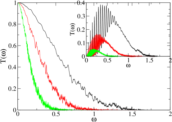
Figure 2: (color online) $1D$ unpinned case with both free and fixed (INSET) boundary conditions: plot of the disorder averaged transmission $T(\omega)$ versus $\omega$ for $\Delta=0.4$. The various curves (from top to bottom) correspond to lattices of sizes $N=64,256,1024$ respectively.

In Fig. (2) we plot numerical results showing ${T}_{N}(\omega)$ for the $1D$ binary mass-disordered lattice with both fixed and free boundary conditions. One can clearly see the two features discussed above namely (i) dependence of frequency cut-off on system size and (ii) dependence of form of ${T}_{N}(\omega)$ on boundary conditions. Using the three observations made above it is easy to arrive at the conclusion that $J\sim N^{-3/2}$ for fixed BC and $J\sim N^{-1/2}$ for free BC. In the presence of a pinning potential the low-frequency modes are suppressed and one obtains a heat insulator with $J\sim e^{-cN}$, with $c$ a constant oconnor74 (see also dharleb08 and references there).

Higher dimensions. Let us try to extend the analysis of the $1D$ case to higher dimensions. For this we will use inputs from both kinetic theory and the theory of phonon localization. The main point of our arguments involves the assumption that normal modes can be classified as ballistic, diffusive or localized. Using localization theory we determine the frequency region where states are localized. The lowest frequency states with $\omega\to 0$ will be ballistic and we use kinetic theory to determine the fraction of extended states which are ballistic. We assume that at sufficiently low frequencies the effective disorder is always weak (even when the mass variance $\Delta$ is large) and one can still use kinetic theory. Corresponding to the three observations made above for the $1D$ case we now make the following arguments:

(i) From localization theory one expects all fixed non-zero frequency states in a $2D$ disordered system to be localized when the size of the system goes to infinity. As discussed in Sec. (I) localization theory gives us a frequency cut-off $\omega_{c}^{L}=(\ln N)^{-1/2}$ in $2D$ above which states are localized. In $3D$ one obtains a finite frequency cut-off $\omega_{c}^{L}$ independent of system size above which states are localized.

(ii) For the unpinned case with finite $N$ there will exist low frequency states below $\omega_{c}^{L}$, in both $2D$ and $3D$, which are extended states. These states are either diffusive or ballistic. Ballistic modes are insensitive to the disorder and their transmission coefficient are almost the same as for the ordered case. To find the frequency cut-off below which states are ballistic we use kinetic theory results (see Appendix A). For the low-frequency extended states we expect kinetic theory to be reliable and this gives us a mean free path for phonons $\ell_{K}\sim\omega^{-(d+1)}$. This means that for low frequencies $\omega\stackrel{{\scriptstyle<}}{{\sim}}\omega_{c}^{K}=N^{-1/(d+1)}$ we have $\ell_{K}(\omega)>N$ and phonons transmit ballistically. We now proceed to calculate the contribution of these ballistic modes to the total current. This can be obtained by looking at the small $\omega$ form of $T_{N}(\omega)$ for the ordered lattice.

(iii) For the ordered lattice $T_{N}(\omega)$ is typically a highly oscillatory function with the oscillations increasing with system size. An effective transmission coefficient in the $N\to\infty$ limit can be obtained by considering the integrated transmission. This asymptotic effective low-frequency form of $T_{N}(\omega)$, for the ordered lattice can be calculated using methods described in roydhar08 and is given by:

$$T(\omega) \sim \omega^{d+1}~{},~{}~{}~{}~{}~{}{\rm fixed~{}BC}$$

$$T(\omega) \sim \omega^{d-1}~{},~{}~{}~{}~{}~{}~{}{\rm free~{}BC}~{},$$ (12)

the result being valid for $d=1,2,3$ anupam09 .

Using the above arguments we then get the ballistic contribution to the total current density (for the unpinned case) as:

$$J_{\rm ball} \sim \int_{0}^{\omega_{c}^{K}}d\omega~{}\omega^{d+1}\sim\frac{1}{N^{(d+2)/(d+1)}}~{},~{}~{}~{}~{}{\rm fixed~{}~{}BC,}$$ (13)

$$\sim \int_{0}^{\omega_{c}^{K}}d\omega~{}\omega^{d-1}\sim\frac{1}{N^{d/(d+1)}}~{},~{}~{}~{}~{}{\rm free~{}~{}BC}~{}.~{}~{}~{}$$

We can now make predictions for the asymptotic system size dependence of total current density in two and three dimensions.

Two dimensions: From localization theory one expects that all finite frequency modes $\omega\stackrel{{\scriptstyle>}}{{\sim}}\omega_{c}^{L}=(\ln N)^{-1/2}$ are localized and their contribution to the total current falls exponentially with system size. Our kinetic theory arguments show that the low frequency extended states with $\omega_{c}^{K}\stackrel{{\scriptstyle<}}{{\sim}}\omega\stackrel{{\scriptstyle<}}{{\sim}}\omega_{c}^{L}$ are diffusive (where $\omega_{c}^{K}=N^{-1/3}$) while the remaining modes with $\omega\stackrel{{\scriptstyle<}}{{\sim}}\omega_{c}^{K}$ are ballistic. The diffusive contribution to total current will then scale as $J_{\rm diff}\sim(\ln N)^{-1/2}N^{-1}$. The ballistic contribution depends on BCs and is given by Eq. (13). This gives $J_{\rm ball}\sim N^{-4/3}$ for fixed BC and $J_{\rm ball}\sim N^{-2/3}$ for free BC. Hence, adding all the different contributions, we conclude that asymptotically:

$$J \sim \frac{1}{(\ln N)^{1/2}N}~{},~{}~{}~{}~{}{\rm fixed~{}~{}BC,}~{}~{}d=2~{},$$ (14)

$$\sim \frac{1}{N^{2/3}}~{},~{}~{}~{}~{}~{}~{}~{}{\rm free~{}~{}BC,}~{}~{}d=2.$$

In the presence of an onsite pinning potential at all sites the low frequency modes get cut off and all the remaining states are localized, hence we expect:

$$J\sim e^{-bN},~{}~{}~{}~{}~{}~{}~{}~{}~{}~{}~{}{\rm pinned}~{},~{}~{}d=2~{},$$ (15)

where $b$ is some positive constant.

Three dimensions: In this case localization theory tells us that modes with $\omega\stackrel{{\scriptstyle>}}{{\sim}}\omega_{c}^{L}$ are localized and $\omega_{c}^{L}$ is independent of $N$. From kinetic theory we find that the extended states with $\omega_{c}^{K}\stackrel{{\scriptstyle<}}{{\sim}}\omega\stackrel{{\scriptstyle<}}{{\sim}}\omega_{c}^{L}$ are diffusive (with $\omega_{c}^{K}=N^{-1/4}$) and those with $\omega\stackrel{{\scriptstyle<}}{{\sim}}\omega_{c}^{K}$ are ballistic. The contribution to current from diffusive modes scales as $J_{\rm diff}\sim N^{-1}$. The ballistic contribution (from states with $\omega\stackrel{{\scriptstyle<}}{{\sim}}N^{-1/4}$) is obtained from Eq. (13) and gives $J_{\rm ball}\sim N^{-5/4}$ for fixed BC and $J_{\rm ball}\sim N^{-3/4}$ for free BC. Hence, adding all contributions, we conclude that asymptotically:

$$J \sim \frac{1}{N}~{},~{}~{}~{}~{}~{}~{}{\rm fixed~{}~{}BC~{},}~{}~{}d=3~{},$$ (16)

$$\sim \frac{1}{N^{3/4}}~{},~{}~{}~{}~{}~{}~{}{\rm free~{}~{}BC~{},}~{}~{}d=3~{}.$$

In the presence of an onsite pinning potential at all sites the low frequency modes get cut off and, since in this case the remaining states form bands of diffusive and localized states, hence we expect:

$$J\sim\frac{1}{N}~{},~{}~{}~{}~{}~{}~{}~{}{\rm pinned~{},}~{}~{}d=3.$$ (17)

Thus in $3D$ both the unpinned lattice with fixed boundary conditions and the pinned lattice are expected to show Fourier type of behaviour as far as the system size dependence of the current is considered.

Note that for free BC, the prediction for the current contribution from the ballistic part $J_{\rm ball}\sim N^{-d/(d+1)}$ is identical to that from kinetic theory discussed in Sec. (I). This agreement can be traced to the small $\omega$ form of $T(\omega)\sim\omega^{d-1}$ for free BC [see Eq. (12)] which is identical to the form of the density of states $\rho(\omega)$ used in kinetic theory. The typical form of density of states for ordered and disordered lattices in different dimensions is shown in Fig. (3) and we can see that the low frequency form is similar in both cases and has the expected $\omega^{d-1}$ behaviour. However it seems reasonable to expect that, since the transport current phonons are injected at the boundaries, in kinetic theory one needs to use the local density of states evaluated at the boundaries. For fixed BC this will then give rise to an extra factor of $\omega^{2}$ (from the squared wavefunction) and then the kinetic theory prediction matches with those given above.

We note that the density of states in Fig. (3) show apparent gaps in the middle ranges of $\omega$ for $d=2,3$. These might be expected to disappear when the size of the system goes to infinity when there should be large regions containing only masses of one type casher71 ; oconnor74 . These regions will however be rare. In Fig. (4) we show plots of the density of states for the ordered and disordered harmonic lattices in the presence of pinning. In this case the gaps in the spectrum are more pronounced and, for large enough values of $k_{o}$ and $\Delta$, may be present even in the thermodynamic limit.

IV Results from Numerics and Simulations

We now present the numerical and simulation results for transmission coefficients, heat current density, temperature profiles and IPRs for the disordered harmonic lattice in various dimensions. The numerical scheme for calculating $J$ is both faster and more accurate than nonequilibrium simulations. Especially, for strong disorder, equilibration times in nonequilibrium simulations become very large and in such cases only the numerical method can be used. However we also show some nonequilibrium simulation results. Their almost perfect agreement with the numerical results provides additional confidence in the accuracy of our results. In Sec. (IV.1) we give the results for the $2D$ lattice for the unpinned case with both fixed and free boundary conditions and then for the pinned case. In Sec. (IV.2) we present the results for the three dimensional case with and without substrate pinning potentials.

IV.1 Results in two dimensions

In this section we consider $N\times N$ square lattices with periodic BCs in the $\nu=2$ direction and either fixed or free BCs in the conducting direction ($\nu=1$). One of the interesting questions here is as to how the three properties for the $1D$ case discussed in Sec. (III) get modified for the $2D$ case.

IV.1.1 Disordered $2D$ lattice without pinning

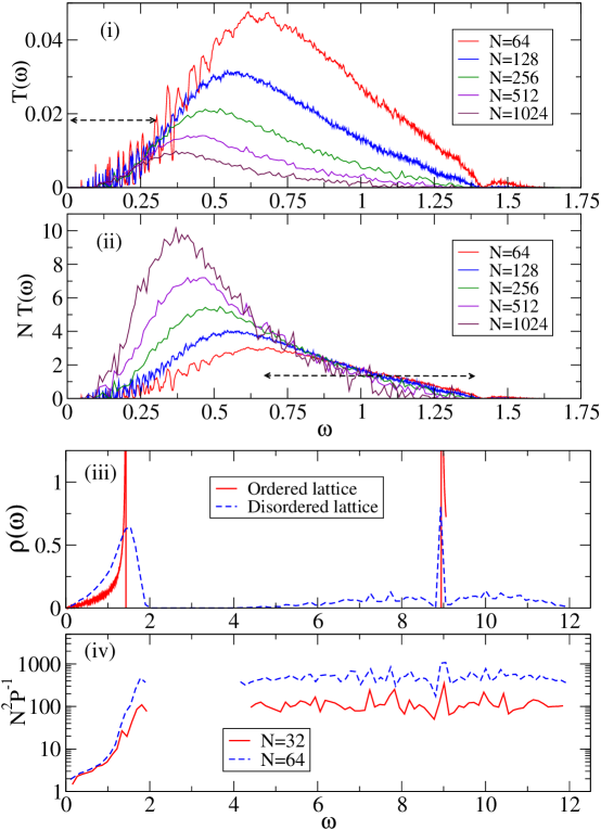
Figure 5: (color online) $2D$ unpinned case with fixed BC for $\Delta=0.95$. (i) Plot of the disorder averaged transmission $T(\omega)$ versus $\omega$. (ii) Plot of $NT(\omega)$. The range of frequencies for which $T(\omega)\sim 1/N$ is indicated by the dashed line. (iii) Plot of $\rho(\omega)$ for binary mass ordered and single disordered sample. (iv) Plot of $N^{2}P^{-1}$ for single samples (smoothed data). We see that even though the allowed normal modes occur over a large frequency band $\approx(0-12)$, transmission takes place in a small band $\approx(0-1.25)$ and is negligible elsewhere. The IPR plots confirm that the non-transmitting states correspond to localized modes. In (i) we see that $\omega_{c}^{L}$ is slowly decreasing with inrease of $N$.

Fixed BC: we have computed the transmission coefficients and the corresponding heat currents for different values of $\Delta$ and for system sizes from $N=16-1024$. The number of averages varied from over $100$ samples for $N=16$ to about two samples for $N=1024$. In Figs. (5,6,7) we plot the disorder averaged transmission coefficient for three different disorder strengths, $\Delta=0.95$, $\Delta=0.8$ and $\Delta=0.2$, for different system sizes. The corresponding plots of IPRs as a function of normal mode frequency $\omega_{p}$, for single disorder realizations, are also given. From the IPR plots we get an idea of the typical range of allowed normal mode frequencies and their degree of localization. Low IPR values which scale as $N^{-2}$ imply extended states while large IPR values which do not change much with system size denote localized states. In Fig. (6) we also show typical plots of small IPR and large IPR wavefunctions. From Figs. (5,6,7) we make the following observations:

(i) As expected we see significant transmission only over the range of frequencies with extended states. Thus in Fig. (5) for $\Delta=0.95$ we see that, while there are normal modes in the range $\omega\approx(0-12)$, transmission is appreciable only in the range $\omega\approx(0-1.5)$ and this is also roughly the range where the IPR data shows a $N^{-2}$ scaling behaviour. This can also be seen in Fig. (6) where the inset shows the decay of $T(\omega)$ in the localized region. Unlike the $1D$ case we see a very weak dependence on system size of the upper frequency cut-off $\omega_{c}^{L}$ beyond which states are localized and transmission is negligible. As discussed earlier, localization theory predicts $\omega_{c}^{L}\sim(\ln N)^{-1/2}$ but this may be difficult to observe numerically. The overall transmission function ${T}_{N}(\omega)$ decreases with increasing system size, with $T(\omega)\sim 1/N$ at higher freqencies and $T(\omega)\sim N^{0}$ at the lowest frequencies.

(ii) In Fig. (7) we have also plotted $T(\omega)$ for the ordered binary mass case and we note that over a range of small frequencies, $T(\omega)$ for the disordered case is very close to the curve for the ordered case, which means that these modes are ballistic. As expected from the arguments in Sec. (III) we roughly find $T(\omega)\sim\omega^{3}$ at small frequencies. The remaining transmitting states are either diffusive (with a $1/N$ scaling) or are in the cross-over regime between diffusive and ballistic and so do not have a simple scaling.

We next look at the the integrated transmission which gives the net heat current. The system size dependence of the disorder averaged current $J$ for different values of $\Delta$ is shown in Fig. (8). For the case $\Delta=0.2$, we also show simulation results and one can see that there is excellent agreement with the numerical results. For $\Delta=0.2$ we get an exponent $\mu\approx 0.6$ which is close to the value obtained earlier in lee05 for a similar disorder strength. However with increasing disorder we see that this value changes and seems to settle to around $\mu\approx 0.75$. It seems reasonable to expect (though we have no rigorous arguments) that there is only one asymptotic exponent and for small disorder one just needs to go to very large system sizes to see the true value. In Fig. (9) we show temperature profiles obtained from simulations for lattices of different sizes with $\Delta=0.2$. The jumps at the boundaries indicate that the asymptotic size limit has not yet been reached. This is consistent with our result that the exponent $\mu$ obtained at $\Delta=0.2$ is different from what we believe is the correct asymptotic value (obtained at larger values of $\Delta$). We do not have temperature plots at strong disorder where simulations are difficult.

Thus contrary to the arguments in Sec. (III) which predicted $J\sim(\ln N)^{-1/2}N^{-1}$ we find a much larger current scaling as $J\sim N^{-0.75}$. It is possible that one needs to go to larger system sizes to see the correct scaling.

Free BC: In this case from the arguments in Sec. (III) we expect ballistic states to contribute most significantly to the current density giving $J\sim N^{-2/3}$.

In Figs. (10,11) we plot the disorder averaged transmission coefficient for $\Delta=0.8$ and $\Delta=0.2$ for different system sizes. Qualitatively these results look very similar to those for fixed boundaries. However transmission is now significantly larger in the region of extended states. The behaviour at frequencies $\omega\to 0$ is also different and we now find $T(\omega)\sim\omega$ in contrast to $T(\omega)\sim\omega^{3}$ for fixed boundaries. From the plots of IPRs in Fig. (10) we note that there is not much qualitative difference with the fixed boundary plots except in the low frequency region (see below).

The system size dependence of the disorder averaged current $J$ for two different values of $\Delta$ is shown in Fig. (12). For $\Delta=0.2$ we get an exponent $\mu\approx 0.5$ while for the stronger disorder case $\Delta=0.8$ we see a different exponent $\mu\approx 0.6$. Again we believe that the strong disorder value of $\mu=0.6$ is closer to the value of the true asymptotic exponent. This value is close to the expected $\mu=2/3$ for free BC and significantly different from the value obtained for fixed BC ($\mu\approx 0.75$). Thus the dependence of the value of $\sigma$ on boundary conditions exists even in the $2D$ case.

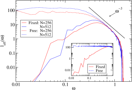
Figure 13: Plot of the effective mean-free path $l_{\rm eff}=NT(\omega)/\omega^{d-1}$ in $2D$ with $\Delta=0.8$. The insets show $\ell_{\rm eff}$ for the ordered lattices with a single mass. An $\omega^{-3}$ behaviour is observed in a small part of the diffusive region.The fixed BC data is highly oscillatory and has been smoothed.

For the case of free BCs, we find that the values of $T(\omega)$ in the diffusive regime matches with those for fixed BCs but are completely different in the ballistic regime. This is seen in Fig. (13) where we plot the effective mean free path $l_{\rm eff}(\omega)=NT(\omega)/w^{d-1}$ in the low-frequency region [this is obtained by comparing Eq. (6) with the kinetic theory expression for conductivity Eq. (2)]. For free BC, $l_{\rm eff}$ is roughly consistent with the kinetic theory prediction $l^{-1}_{\rm eff}\sim N^{-1}+{\ell_{K}}^{-1}(\omega)$ but the behaviour for fixed BC is very different. The inset of Fig. (13) plots $l_{\rm eff}$ for the equal mass ordered case and we find that in the ballistic regime it is very close to the disordered case, an input that we used in the heuristic derivation. The numerical data also confirms that for small $\omega$, $T(\omega)\sim\omega$ for free BCs and as $\omega^{3}$ for fixed BCs. The transmission for fixed BC shows rapid oscillations which increase with system size, and arise from scattering and interference of waves at the interfaces.

IV.1.2 Disordered $2D$ lattice with pinning

We now study the effect of introducing a harmonic pinning potential at all sites of the lattice. It is expected that this will cut off low frequency modes and hence one should see strong localization effects. The localization length $\ell$ will decrease both with increasing $\Delta$ and increasing $k_{o}$ (in $1D$ heuristic arguments give $\ell\sim 1/(\Delta^{2}k_{o})$ dharleb08 ). In Figs. (14,15) we plot the transmission coefficients for two cases with on-site potentials $k_{o}=10.0$ and $k_{o}=2.0$ respectively, and $\Delta=0.4$. We also plot the IPR in Fig. (14). Unlike in the unpinned case we now find that the transmission coefficients are much smaller and fall more rapidly with system size.

From the plot of $P^{-1}$ we find that for all the modes, the value of $P^{-1}$ does not change much with system size which implies that all modes are localized. The allowed frequency bands correspond to the transmission bands. The two wavefunctions plotted in Fig. (14) correspond to one relatively small and one large $P^{-1}$ value and clearly show that both states are localized.

The system size dependence of the integrated current is shown in Fig. (16) for the two parameter sets. The values of $\mu\approx 1.6,~{}3.65$ for the two sets indicate that at large enough length scales one will get a current falling exponentially with system size and hence we have an insulating phase. In Fig. (17) we plot the temperature profiles for the set with $\Delta=0.4,k_{o}=10.0$ . In this case it is difficult to obtain steady state temperature profiles from simulations for larger system sizes. The reason is that the temperature (unlike current) gets contributions from all modes (both localized and extended) and equilibrating the localized modes takes a long time.

IV.2 Results in three dimensions

In this section we mostly consider $N\times N\times N$ lattices with periodic boundary conditions in the $\nu=2,3$ directions. Some results for $N\times N_{2}\times N_{3}$ lattices with $N_{2}=N_{3}<N$ will also be described. Preliminary results for the case of free BCs are given and indicate that there is no dependence of the exponent $\mu$ on BCs. It is not clear to us whether this is related to the boundedness of the fluctuations in $x_{\bf{n}}$ and the decay of the correlations between $x_{\bf{n}}$ and $x_{\bf{l}}$ (like $|{\bf{n}}-{\bf{l}}|^{-1}$) in $d=3$ and their growth (with $N$) in $d<3$.

IV.2.1 Disordered $3D$ lattice without pinning

Fixed BC: we have used both the numerical approach and simulations for sizes up to $32\times 32\times 32$ for which we have data for $T(\omega)$. For larger systems the matrices become too big and we have not been able to use the numerical approach. Hence, for larger system sizes we have only performed simulations, including some on $N\times N_{2}\times N_{2}$ lattices. For these cases only the current $J$ is obtained. The number of averages varies from over $100$ samples for $N=16$ to two samples for $N=64$. In Figs. (18,19) we plot the disorder averaged transmission coefficient for two different disorder strengths, $\Delta=0.8$ and $\Delta=0.2$, for different system sizes. The corresponding plots of IPRs as a function of normal mode frequency $\omega_{p}$, for single disorder realizations, are also given. From the IPR plots we get an idea of the typical range of allowed normal mode frequencies and their degree of localization. Low IPR values which scale as $N^{-3}$ imply extended states while large IPR values which do not change much with system size denote localized states.

From Figs. (18,19) we make the following observations.

(i) From the $3D$ data it is clear the effect of localization is weaker than in $1D$ and $2D$. Both for $\Delta=0.2$ and $\Delta=0.8$ we find that there is transmission over almost the entire range of frequencies of the allowed normal modes. From the IPR plots we see that for $\Delta=0.2$ most states are extended except for a small region in the high frequency band-edge. For $\Delta=0.8$ the allowed modes form two bands and one finds significant transmission over almost the full range. At the band edges (except the one at $\omega=0$) there are again localized states. It also appears that there are some large IPR states interspersed within the high frequency band. As in the $2D$ case and unlike the $1D$ case, the frequency range over which transmission takes place does not change with system size, only the overall magnitude of transmission coefficient changes.

(ii) The plot of $NT(\omega)$ in Fig. (18) shows the nature of the extended states. The high frequency band and a portion of the lower frequency band have the scaling $T(\omega)\sim N^{-1}$ and hence corresponds to diffusive states. In the lower-frequency band the fraction of diffusive states seems to be increasing with system size but it is difficult to verify the $\omega_{c}^{K}\sim N^{-1/4}$ scaling. The ballistic nature of the low-frequency states is confirmed in Fig. (19) where we see that $T(\omega)$ for the binary-mass ordered and disordered lattices match for small $\omega$ [with a $T(\omega)\sim\omega^{4}$ dependence].

In Fig. (20) we show the system size dependence of the disorder averaged current density $J$ for the two cases with weak disorder strength ($\Delta=0.2$) and strong disorder strength ($\Delta=0.8$). The results for cubic lattices of sizes up to $N=32$ are from the numerical method while the results for larger sizes are from simulations. We find an exponent $\mu\approx 0.6$ at small disorder and $\mu\approx 0.75$ at large disorder strength. As in the $2D$ case here too we believe that at small disorder, the asymptotic system size limit will be reached at much larger system sizes and that the exponent obtained at large disorder strength is probably close to the true asymptotic value. The value ($\mu=0.75$) does not agree with the prediction ($J\sim N^{-1}$) made from the heuristic arguments in Sec. (III). A study of larger system sizes is necessary to confirm whether or not the asymptotic size limit has been reached.

The data point at $N=128$ for the set with $\Delta=0.2$ in Fig. (20) actually corresponds to a lattice of dimensions $128\times 48\times 48$ and we believe that the current value is very close to the expected fully $3D$ value. To see this point, we have plotted in Fig. (21) results from nonequilibrium simulations with $N\times N_{2}\times N_{2}$ lattices with $N_{2}\leq N$.

Finally, in Fig. (22) we show temperature profiles (for single disorder realizations) obtained from simulations for lattices of different sizes and with $\Delta=0.2$. The jumps at the boundaries again indicate that the asymptotic system size limit has not been reached even at the largest size.

Free BC: In this case from the arguments in Sec. (III) we expect ballistic states to contribute most significantly to the current density giving $J\sim N^{-3/4}$.

In Fig. (23) we plot the disorder averaged transmission coefficient for $\Delta=0.8$ for different system sizes. The transmission function is very close to that for the fixed boundary case except in the frequency region corresponding to non-diffusive states. At $\omega\to 0$ we now expect, though it is hard to verify from the data, that $T(\omega)\sim\omega^{2}$ in contrast to $T(\omega)\sim\omega^{4}$ for fixed boundaries.

The system size dependence of the disorder averaged current $J$ for two different values of $\Delta$ is shown in Fig. (20). We find that the current values are quite close to the fixed BC case and the exponent obtained at the largest system size studied for this case is $\mu\approx 0.71$. This value is close to the expected $\mu=3/4$ for free BC.

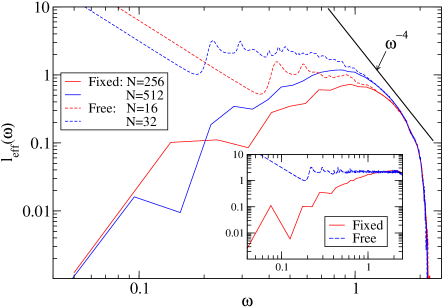
Figure 24: Plot of the effective mean-free path $l_{\rm eff}=NT(\omega)/\omega^{d-1}$ in $3D$ with $\Delta=0.8$ for fixed and free BCs. The insets show $\ell_{\rm eff}$ for the ordered system with a single mass. An $\omega^{-4}$ behaviour is observed in a small part of the diffusive region.The fixed BC data is highly oscillatory and has been smoothed.

We now compare the transmission coefficient for free and fixed BCs in the ballistic regime. This is plotted in Fig. (24) where we show the effective mean free path $l_{\rm eff}(\omega)=NT(\omega)/w^{d-1}$ in the low-frequency region. As in the $2D$ case we again find that for free BCs, $l_{\rm eff}$ is roughly consistent with the kinetic theory prediction $l^{-1}_{\rm eff}\sim N^{-1}+{\ell_{K}}^{-1}(\omega)$ and the behaviour for fixed BCs is very different. The inset of Fig. (24) plots $l_{\rm eff}$ for the equal mass ordered case and we find that in the ballistic regime it is very close to the disordered case. The numerical data confirms the input in our theory on the form of $T(\omega)$ for small $\omega$, i.e.  $T(\omega)\sim\omega^{2}$ for free BCs and as $\omega^{4}$ for fixed BCs. The transmission for fixed BC shows rapid oscillations which increase with system size, and arise from scattering and interference of waves at the interfaces.

IV.2.2 Disordered $3D$ lattice with pinning

For the pinned case, we again use both the numerical method and simulations for sizes up to $N=32$. For $N=64$ only nonequilibrium simulation results are reported.

In Figs. (25,26) we plot the disorder averaged transmission coefficient for $\Delta=0.2$ and $\Delta=0.8$ with $k_{o}=10.0$. The corresponding IPRs $P^{-1}$ and scaled IPRs $N^{3}P^{-1}$ are also shown.

From the IPR plots we notice that the spectrum of the $3D$ disordered pinned chain has a similar interesting structure as in the $2D$ case with two bands and a gap which is seen at strong disorder. However unlike the $2D$ case where all states were localized, here the IPR data indicates that most states except those at the band edges are diffusive. We see localized states at the band edges and also there seem to be some localized states interspersed among the extended states within the bands. The insets in Figs. (25,26) show that there is a reasonable $N^{-1}$ scaling of the transmission data in most of the transmitting region. This is clearer at the larger system sizes. Thus, unlike the unpinned case where low frequency extended states were ballistic or super-diffusive, here we find that there is no transmittance at small ($\omega\to 0$) frequencies and that all states are diffusive.

From the above discussion we expect Fourier’s law to be valid in the $3D$ pinned disordered lattice. The system size dependence of the disorder averaged current $J$ for different disorder strengths is plotted in Fig. (27). For all the parameter sets the exponent obtained is close to $\mu=1$ corresponding to a finite conductivity and validity of Fourier’s law. The temperature profiles plotted in Fig. (28) have small boundary temperature jumps and indicate that the asymptotic size limit has already been reached.

One might expect that at very strong disorder, all states should become localized and then one should get a heat insulator. The parameter set corresponding to Fig. (26) corresponds to strong disorder and for this we still find a significant fraction of extended states. Thus for the binary mass case it appears that there are always extended states. We have some results for the case with a continuous mass distribution ( masses are chosen from a uniform distribution between $1-\Delta$ and $1+\Delta$). In this case we find that the effect of disorder is stronger and the transmission at all frequencies is much reduced compared to the binary mass case. However we cannot see the exponential decrease in transmission with system size and so it is not clear if an insulating behaviour is obtained. Further numerical studies are necessary to understand the asymptotic behaviour.

V Discussion

	$d=2$		$d=3$
	Analytical	Numerical	Analytical	Numerical
Pinned	$\exp{(-bN)}$	$N^{-3.7}$	$N^{-1}$	$N^{-1.0}$
Fixed	$N^{-1}(\ln{N})^{-1/2}$	$N^{-0.75}$	$N^{-1}$	$N^{-0.75}$
Free	$N^{-2/3}$	$N^{-0.6}$	$N^{-3/4}$	$N^{-0.71}$

Table 1: The table summarizes the main results of the paper. The numerical (and nonequilibrium simulation) results obtained in the paper are compared, in two and three dimensions, with the analytical predictions obtained from our heuristic arguments. The error bar for the numerically obtained exponent values is of the order $\pm 0.02$. This error is estimated from the errors in the last few points of the $J$-versus-$N$ data. NB: The system sizes used may well be far from asymptotic.

We have studied heat conduction in isotopically disordered harmonic lattices with scalar displacements in two and three dimensions. The main question addressed is the system size dependence of the heat current, which is computed using Green’s function based numerical methods as well as nonequilibrium simulations. We have tried to understand the size dependence by looking at the phonon transmission function $T(\omega)$ and examining the nature of the energy transport in different frequency regimes. We also described a heuristic analytical calculation based on localization theory and kinetic theory and compared their predictions with our numerical and simulation results. This comparison is summarized in Table (1).

The most interesting findings of this work are:
(i) For the unpinned system we find that in $2D$ there are a large number of localized modes for which phonon transmission is negligible. In $3D$ the number of localized modes is much smaller. The extended modes are either diffusive or ballistic. Our analytic arguments show that the contribution of ballistic modes to conduction is dependent on BCs and is strongly suppressed for the case of fixed BCs, the more realistic case. In $3D$ this leads to diffusive modes dominating for large system sizes and Fourier’s law is satisfied. Thus a finite heat conductivity is obtained for the $3D$ disordered harmonic crystal without the need of invoking anharmonicity as is usually believed to be necessary callaway59 ; ziman72 . This is similar to what one obtains when one adds stochasticity to the time evolution in the bulk as shown by basile06 . Our numerical results verify the predictions for free BCs and we believe that much larger system sizes are necesary to verify the fixed BC results ( this is also the case in $1D$ dhar01 ; roydhar08 ).
(ii) In two dimensions the pinned disordered lattice shows clear evidence of localization and we obtain a heat insulator with exponential decay of current with system size.
(iii) Our result for the $3D$ pinned disordered lattice provides the first microscopic verification of Fourier’s law in a three dimensional system. For the binary mass distribution we do not see a transition to insulating behaviour with increasing disorder. For a continuous mass distribution we find that the current is much smaller (than the binary mass case with the same value of $\Delta$) but it is not clear whether all states get localized and if an insulating phase exists.

Acknowledgements: We thank G. Baskaran, Michael Aizenman, Tom Spencer and especially David Huse for useful discussions. We also thank Srikanth Sastry and Vishwas Vasisht for use of computational facilities. The research of J. L. Lebowitz was supported by NSF grant No. DMR0802120 and by AFOSR grant No. FA9550-07.

Appendix A KINETIC THEORY

Kinetic theory becomes valid in the limit of small disorder. Its basic object is the Wigner function, $f$, which describes the phonon density in phase space and is governed by the transport equation

$$\frac{\partial}{\partial t}f(r,k,t)+\nabla\omega(k)\cdot\nabla_{r}f(r,k,t)=\mathcal{C}f(r,k,t)\,.$$ (18)

Here $r\in\mathbb{R}^{d}$ (boundary conditions could be imposed), $k\in[-\pi,\pi]^{d}$ is the wave number of the first Brioullin zone, $\omega$ is the dispersion relation of the constant mass harmonic crystal, and $\mathcal{C}$ is the collision operator. It acts only on wave numbers and is given by

$$\mathcal{C}f(k)= (2\pi)^{-d+1}\omega(k)^{2}\Delta^{2}\int_{[-\pi,\pi]^{d}}dk^{\prime}$$ (19)

$$\delta\big{(}\omega(k)-\omega(k^{\prime})\big{)}\big{(}f(k^{\prime})-f(k)\big{)}\,.$$

We refer to lukk07 for a derivation. In the range of validity of (18), (19) we can think of phonons as classical particles with energy $\omega$ and velocity $\nabla\omega(k)$. They are scattered by the impurities from $k$ to $dk^{\prime}$ with the rate

$$(2\pi)^{-d+1}\omega(k)^{2}\Delta^{2}\delta\big{(}\omega(k)-\omega(k^{\prime})\big{)}dk^{\prime}.$$ (20)

Collisions are elastic. We distinguish
(i) no pinning potential. Then for small $k$ one has $\omega(k)=|k|$ and $|\nabla\omega(k)|=1$. From (19) the total scattering rate behaves as $|k|^{d+1}$. This is the basis for the discussion in connection with Eq. (2).
(ii) pinning potential. In this case $\omega(k)=\omega_{0}+k^{2}$ for small $k$. The prefactor in (19) can be replaced by $\omega^{2}_{0}$. The velocity is $k$ and the scattering is isotropic with rate $|k|^{d-2}$. Thus the diffusion coefficient results as $D(k)\cong|k|^{-d+4}$ which vanishes as $|k|\to 0$ for $d=2,3$. Hence there is no contribution to the thermal conductivity from the small $k$ modes.

Appendix B Transfer matrix approach

We now outline steps by which $\mathcal{T}_{N}$ can be expressed in forms which are amenable to accurate numerical evaluation. We will give results whereby we express $\mathcal{T}_{N}$ in terms of product of random matrices. These are related to the Green’s function and transfer matrix methods used earlier in the calculation of localization lengths in disordered electronic systems mackinnon83 . Some related discussions for the phonon case can be found in hori68 . For heat conduction in one dimensional disordered chains, the transfer matrix approach has been shown to be very useful in obtaining analytic as well as accurate numerical results and here we study the extension of this to higher dimensions.

The transmission coefficient is given by $\mathcal{T}_{N}(\omega)=4Tr[\mathcal{I}_{L}(\omega)\mathcal{G}^{+}(\omega)\mathcal{I}_{R}(\omega)\mathcal{G}^{-}(\omega)$ where $\mathcal{G}^{+}(\omega)=[-\omega^{2}\mathcal{M}+\mathcal{V}-\mathcal{S}^{+}_{L}-\mathcal{S}^{+}_{R}]^{-1}$, $\mathcal{G}^{-}=[\mathcal{G}^{+}]^{*}$, $\mathcal{I}_{L,R}=Im[\mathcal{S}^{+}_{L,R}]$ and we now specify the form of $\mathcal{S}^{+}_{L,R}$ corresponding to the equations of motion in Eqs. (4). Note that we have transformed to dimensionless variables $\omega\to\omega/\Omega,\mathcal{M}\to\mathcal{M}/\bar{m},~{}\mathcal{V}\to\mathcal{V}/k,~{}\gamma\to\gamma/(\bar{m}\Omega)$ where $\Omega=(k/\bar{m})^{1/2}$. We are considering heat conduction in the $\nu=1$ direction of a $d$-dimensional lattice with particles on the layers $n_{1}=1$ and $n_{1}=N$ being connected to heat baths at temperatures $T_{L}$ and $T_{R}$ respectively. The matrices $\mathcal{S}^{+}_{L}$ and $\mathcal{S}^{+}_{R}$ represent the coupling of the system to the left and right reservoirs respectively, and can be written as $N\times N$ block matrices where each block is a $N^{\prime}\times N^{\prime}$ matrix. The block structures are as follows:

$$\mathcal{S}^{+}_{L}=\left(\begin{array}[]{cccc}{\Sigma_{L}^{+}}&0&...&0\\ 0&0&.~{}.~{}.&0\\ 0&0&.~{}.~{}.&0\end{array}\right)~{},\mathcal{S}^{+}_{R}=\left(\begin{array}[]{cccc}0&0&.~{}.~{}.&0\\ 0&0&.~{}.~{}.&0\\ 0&0&...&\Sigma_{R}^{+}\end{array}\right)~{},~{}~{}$$ (27)

where

$$\Sigma^{+}_{L}=\Sigma^{+}_{R}=i\gamma\omega I~{},$$ (28)

$I$ is a $N^{\prime}\times N^{\prime}$ unit matrix, and $0$ is a $N^{\prime}\times N^{\prime}$ matrix with all elements equal to zero. Similarly the matrices $\mathcal{M}$ and $\mathcal{V}$ have the following block structure:

$$\mathcal{M}=\left(\begin{array}[]{cccc}M_{1}&0&...&0\\ 0&M_{2}&.~{}.~{}.&0\\ 0&0&.~{}.~{}.&0\\ 0&0&.~{}.{}&M_{N}\end{array}\right),~{}\mathcal{V}=\left(\begin{array}[]{cccc}\Phi&-I&.~{}.~{}.&0\\ -I&\Phi&.~{}.~{}.&0\\ 0&0&.~{}.~{}.&0\\ 0&0&..-I{}&\Phi\end{array}\right),~{}~{}$$ (37)

where $M_{n}$ denotes the diagonal mass-matrix for the $n_{1}=n$ layer and $\Phi$ is a force-constant matrix whose off-diagonal terms correspond to coupling to sites within a layer. Hence the matrix $\mathcal{G}^{-1}=[-\mathcal{M}\omega^{2}+\mathcal{V}-\mathcal{S}_{L}^{+}-\mathcal{S}^{+}_{R}]$ has the following structure:

$$[\mathcal{G}]^{-1}=\left(\begin{array}[]{ccccc}a_{1}&-I&0&...&0\\ -I&a_{2}&-I&0~{}...&0\\ ...&...&...&...&...\\ 0&...~{}0&-I&~{}a_{N-1}&-I\\ 0&...&0&-I&a_{N}\end{array}\right)~{},$$ (43)

where $a_{l}=-M_{l}\omega^{2}+\Phi-\delta_{l,1}\Sigma^{+}_{L}-\delta_{l,N}\Sigma^{+}_{R}$. Now defining $\Gamma_{L,R}=Im[\Sigma^{+}_{L,R}]$ and with the form of $\mathcal{S}^{+}_{L,R}$ given in Eqs. (27),(28), we find that the expression for the transmission coefficient reduces to the following form:

$${\mathcal{T}}_{N}(\omega) = 4~{}Tr[{\Gamma}_{L}(\omega){G}^{+}_{N}(\omega){\Gamma}_{R}(\omega){G}^{-}_{N}(\omega)]~{},$$ (44)

where $G^{+}_{N}$ is the $(1,N)^{\rm th}$ block element of $\mathcal{G}$ and $G^{-}_{N}=[G^{+}_{N}]^{\dagger}$. We now show that $G^{+}_{N}$ satisfies a simple recursion equation.

We first introduce some notation. Let ${\mathcal{Y}}^{(l,l+n-1)}$ with $1\leq n\leq N-l+1$ denote a $n\times n$ tridiagonal block matrix whose diagonal entries are $a_{l},a_{l+1},...a_{l+n-1}$, where each $a_{l}$ is a $N^{\prime}\times N^{\prime}$ matrix. The off-diagonal entries are given by $-I$. For an arbitrary block matrix $\mathcal{A}^{(l,m)}$, ${\mathcal{A}}^{(l,m)}_{(i,j)}$ will denote the block sub-matrix of $\mathcal{A}^{(l,m)}$ beginning with $i^{\rm th}$ block row and column and ending with the $j^{\rm th}$ block row and column, while ${A}^{(l,m)}_{i,j}$ will denote the ${(i,j)}^{th}$ block element of $\mathcal{A}^{(l,m)}$. Also $\mathcal{I}_{n}$ will denote a $n\times n$ block-diagonal matrix with diagonal elements $I$.

The inverse of ${\mathcal{Y}}^{(1,N)}$ is denoted by $[\mathcal{Y}^{(1,N)}]^{-1}={\mathcal{G}}^{(1,N)}$ and satisfies the equation:

$${\mathcal{Y}}^{(1,N)}~{}{\mathcal{G}}^{(1,N)} = {\mathcal{I}}_{N}~{}.$$

According to our notation we have ${\mathcal{G}}^{(1,N)}=\mathcal{G}^{+}$ and $G^{(1,N)}_{1,N}=G^{+}_{N}$. The matrix $\mathcal{Y}^{(1,N)}$ has the following structure:

$${\mathcal{Y}}^{(1,N)}=\left(\begin{array}[]{cc}{\mathcal{Y}}^{(1,N-1)}&{\mathcal{W}}_{N}\\ {\mathcal{W}}_{N}^{T}&a_{N}\end{array}\right)~{},$$ (47)

where ${\mathcal{W}}_{N}^{T}=(0,0,...,-I)$ is a ${1\times N-1}$ block vector. We then write Eq. (B) in the form

$$\left(\begin{array}[]{cc}{\mathcal{Y}}^{(1,N-1)}&{\mathcal{W}}_{N}\\ {\mathcal{W}}_{N}^{T}&a_{N}\end{array}\right)\left(\begin{array}[]{cc}{\mathcal{G}}^{(1,N)}_{(1,N-1)}&{\mathcal{U}}_{N}\\ {\mathcal{U}}_{N}^{T}&G^{(1,N)}_{N,N}\end{array}\right)=\left(\begin{array}[]{cc}{\mathcal{I}}_{N-1}&0\\ 0&I\end{array}\right),~{}~{}$$ (54)

where ${\mathcal{U}}_{N}^{T}=[G^{(1,N)T}_{1,N},G^{(1,N)T}_{2,N}...,G^{(1,N)T}_{N-1,N}]$ is a $1\times N-1$ block vector. From Eq (54) we get the following four equations:

$${\mathcal{Y}}^{(1,N-1)}~{}{\mathcal{G}}^{(1,N)}_{(1,N-1)}+{\mathcal{W}}_{N}~{}{\mathcal{U}}_{N}^{T}={\mathcal{I}}_{N-1}~{},$$

$${\mathcal{W}}_{N}^{T}~{}{\mathcal{G}}^{(1,N)}_{(1,N-1)}+a_{N}~{}{\mathcal{U}}_{N}^{T}=0~{},$$

$${\mathcal{Y}}^{(1,N-1)}~{}{\mathcal{U}}_{N}+{\mathcal{W}}_{N}~{}G^{(1,N)}_{N,N}=0~{},$$

$${\mathcal{W}}_{N}^{T}~{}{\mathcal{U}}_{N}+a_{N}~{}G^{(1,N)}_{N,N}=I~{}.$$ (55)

Noting that $[\mathcal{Y}^{(1,N-1)}]^{-1}=\mathcal{G}^{(1,N-1)}$ we get, using the third equation above and the form of $\mathcal{W}_{N}$:

$$\mathcal{U}_{N} = -\mathcal{G}^{(1,N-1)}\mathcal{W}_{N}G^{(1,N)}_{N,N}~{},$$

$${\rm or}~{}~{}G^{(1,N)}_{i,N} = {G}^{(1,N-1)}_{i,N-1}G^{(1,N)}_{N,N}~{},~{}{\rm for}~{}~{}i=1,2,...,N-1.~{}~{}~{}~{}$$ (56)

From the fourth equation in Eq. (55) we get:

$$G^{(1,N)}_{N-1,N} = a_{N}~{}G^{(1,N)}_{N,N}-I~{}.$$ (57)

We will now use Eqs. (56),(57) to obtain a recursion for $G^{(1,N)}_{1,N}$ $=G_{N}^{+}$ in Eq. (44)], which is the main object of interest. Let us define $P^{(l,n)}=[G^{(l,n)}_{1,n-l+1}]^{-1}$ where $\mathcal{G}^{(l,m)}=[\mathcal{Y}^{(l,m)}]^{-1}$. Then setting $i=1$ in Eq. (56) and taking an inverse on both sides we get:

$$P^{(1,N)}=[G^{(1,N)}_{N,N}]^{-1}~{}P^{(1,N-1)}.$$ (58)

Setting $i=N-1$ in Eq. (56) we get $G^{(1,N)}_{N-1,N}=G^{(1,N-1)}_{N-1,N-1}G^{(1,N)}_{N,N}$ and using this in Eq. (57) we get $[G^{(1,N)}_{N,N}]^{-1}=[a_{N}-G^{(1,N-1)}_{N-1,N-1}]$ . Inserting this in the above equation we finally get our required recursion relation:

$$P^{(1,N)}=a_{N}P^{(1,N-1)}-P^{(1,N-2)}~{}.$$ (59)

The initial conditions for this recursion are: $P^{(1,0)}=I_{M}$ and $P^{(1,1)}=a_{1}$. By proceeding similarly as before we can also obtain the following recursion relation:

$$P^{(n,N)}=P^{(n+1,N)}a_{1}-P^{(n+2,N)}~{},~{}~{}~{}n=1,2,...,N-1~{},$$ (60)

and $P^{(1,N)}$ can be recursively obtained using the initial conditions $P^{(N+1,N)}=I_{M}$ and $P^{(N,N)}=a_{N}$. Given the set $\{a_{i}\}$, by iterating either of the above equations one can numerically find $P^{(1,N)}$ and then invert it to find $G_{1,N}^{(1,N)}$. However this scheme runs into accuracy problems since the numerical values of the matrix elements of the iterates grow rapidly. We describe now a different way of performing the recursion which turns out to be numerically more efficient. We first define

$$r_{N}=P^{(1,N)}[P^{(1,N-1)}]^{-1}~{}.$$ (61)

From Eq. (59) we immediately get:

$$r_{N}=a_{N}-\frac{1}{r_{N-1}}~{},$$ (62)

with the initial condition $r_{1}=a_{1}$. Then $G_{1,N}^{(1,N)}$ is given by:

$$G_{1,N}^{(1,N)} = [P^{(1,N)}]^{-1}=[r_{N}r_{N-1}...r_{1}]^{-1}$$ (63)

$$= r_{1}^{-1}r_{2}^{-1}...r_{N}^{-1}~{}.$$

This form where at each stage $r_{l}^{-1}$ is evaluated turns out to be numerically more accurate.

Finally we show that one can express $G_{1,N}^{(1,N)}$ in the form of a product of matrices. The product form is such that the system and reservoir contributions are separated. First we note that the form of the matrices $a_{l}$ for our specific problem is: $a_{l}=c_{l}-\delta_{l,1}\Sigma_{1}-\delta_{l,N}\Sigma_{N}$ where $c_{l}=-M_{l}\omega^{2}+\Phi$. We define system-dependent matrices $Q^{(1,n)},~{}Q^{(n,N)}$ by replacing $a_{1},a_{N}$ by $c_{1},c_{N}$ in the recursions for $P$s’. Thus $Q^{(1,n)}=P^{(1,n)}(a_{1}\to c_{1},a_{N}\to c_{N})$ and $Q^{(n,N)}=P^{(n,N)}(a_{1}\to c_{1},a_{N}\to c_{N})$. Clearly $Q$s’ satisfy the same recursion as the $P$s’ with $a_{l}$ replaced by $c_{l}$. Then using Eqs. (59),(60), and similar equations for the $Q$s’ we get:

$$P^{(1,N)}$$ (68)

$$= Q^{(1,N)}-Q^{(2,N)}~{}\Sigma_{1}-\Sigma_{N}~{}Q^{(1,N-1)}+\Sigma_{N}~{}Q^{(2,N-1)}~{}\Sigma_{1}$$

$$= (1~{}~{}~{}-\Sigma_{N})\left(\begin{array}[]{cc}Q^{(1,N)}&-Q^{(2,N)}\\ Q^{(1,N-1)}&-Q^{(2,N-1)}\end{array}\right)\left(\begin{array}[]{c}1\\ \Sigma_{1}\end{array}\right)~{}.$$

From the recursion relations for the $Q$s’ it is easy to see that

$$\left(\begin{array}[]{cc}Q^{(1,N)}&-Q^{(2,N)}\\ Q^{(1,N-1)}&-Q^{(2,N-1)}\end{array}\right)$$ (71)

$$= \left(\begin{array}[]{cc}a_{N}&-I\\ I&0\end{array}\right)\left(\begin{array}[]{cc}Q^{(1,N-1)}&-Q^{(2,N-1)}\\ Q^{(1,N-2)}&-Q^{(2,N-2)}\end{array}\right)$$ (76)

$$= \hat{T}_{N}\hat{T}_{N-1}...\hat{T}_{1}~{},$$ (77)

where

$$\hat{T}_{l} = \left(\begin{array}[]{cc}a_{l}&-I\\ I&0\end{array}\right)~{}.$$ (80)

We then obtain $G^{+}_{N}=[P^{(1,N)}]^{-1}$.

In our numerical calculations we use the recursion relations in Eqs. (62),(63) to evaluate the required Green’s function. Computing the trace in Eq. (44) then gives us the transmission coefficient as a function of frequency.

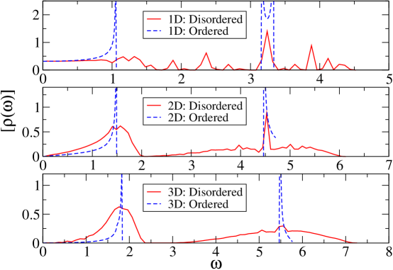
Figure 3: (color online) Unpinned lattices with fixed BC in one direction and periodic in all others.
Disorder averaged density of states obtained numerically from the eigenvalues of several disorder realizations in $1D,2D$ and $3D$ for lattice sizes $N=4096,64,16$ respectively. Note that the low frequency behaviour is unaffected by disorder and one has $\omega^{d-1}$ as $\omega\to 0$. We set $\Delta=0.8,k=1$ and averaged over $30$ realizations in $1D$ and over $10$ realizations in $2D$ and $3D$. In $2D$ and $3D$ there is not much variation in $\rho(\omega)$ for different disorder samples. Also shown are the density of states for the binary mass ordered lattices.

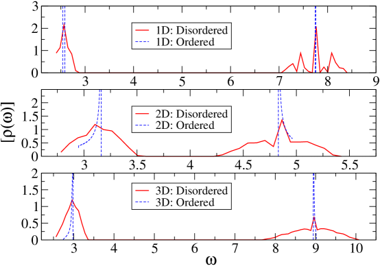
Figure 4: (color online) Pinned lattices.
Disorder averaged density of states obtained numerically from the eigenvalues of several disorder realizations in $1D,2D$ and $3D$ for lattice sizes $N=4096,64,16$ respectively. Note that low frequency modes are absent. We set $k=1,k_{o}=10.0$ and $\Delta=0.4$ in $2D$ and $\Delta=0.8$ in $1D,3D$. Averages were taken over $30$ realizations in $1D$ and $10$ realizations in $2D,3D$. We find that in $2D$ and $3D$ there is not much variation in $\rho(\omega)$ for different disorder samples. Also shown are the density of states for the binary mass ordered lattices.

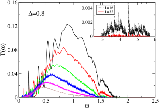
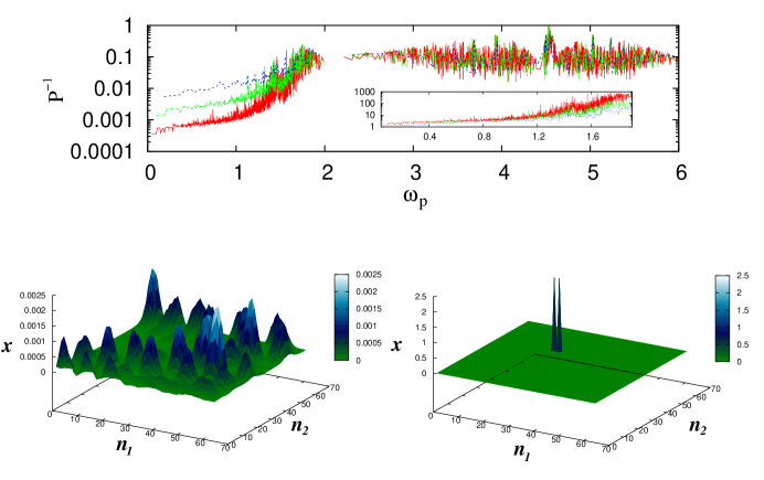
Figure 6: (color online) $2D$ unpinned case with fixed BC for $\Delta=0.8$.
TOP: Plot of the disorder averaged transmission $T(\omega)$ versus $\omega$. The various curves (from top to bottom ) correspond to square lattices with $N=16,32,64,128,256,512$ respectively. We see again that most modes are localized and transmission takes place over a small range of requencies.
BOTTOM: Plot shows the IPR ($P^{-1}$) as a function of normal mode-frequency $\omega_{p}$ for the $2D$ lattice with $\Delta=0.8$. The curves are for $N=16$ (blue), $32$ (green) and $64$ (red). The inset plots $N^{2}P^{-1}$ and the collapse at low frequencies shows that these modes are extended. Also shown are two typical normal modes for one small (left) and one large value of $P^{-1}$ for $N=64$.

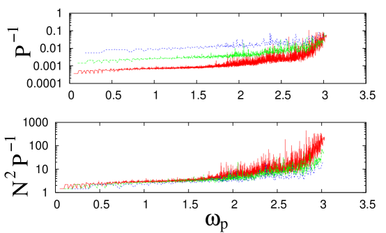
Figure 7: (color online) $2D$ unpinned case with fixed BC for $\Delta=0.2$.
TOP: Plot of the disorder averaged transmission $T(\omega)$ versus $\omega$. The upper-most curve corresponds to a binary-mass ordered lattice with $N=128$ while the remaining curves (from top to bottom) correspond to square lattices with $N=16,32,64,128,256,512$ respectively.
BOTTOM: Plot shows the IPR ($P^{-1}$) and scaled IPR ($N^{2}P^{-1}$) as a function of normal mode-frequency $\omega_{p}$. The curves are for $N=16$ (blue), $32$ (green) and $64$ (red).

Figure 8: (color online) $2D$ unpinned lattice with fixed BC.
Plot of disorder-averaged current $J$ versus system size for different values of $\Delta$. The error-bars show the actual standard deviations from sample-to-sample fluctuations. Numerical errors are much smaller. For $\Delta=0.2$, simulation data is also plotted.

Figure 9: (color online) $2D$ unpinned case with fixed BC for $\Delta=0.2$.
Plot of disorder-averaged temperature profile $[T_{i}]$ for different system sizes obtained from simulations.

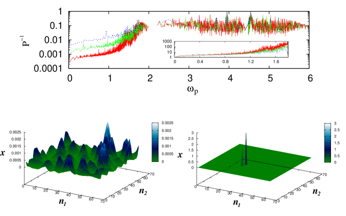
Figure 10: (color online) $2D$ unpinned case with free BC for $\Delta=0.8$.
TOP: Plot of the disorder averaged transmission $T(\omega)$ versus $\omega$. The various curves (from top to bottom) correspond to square lattices with $N=16,32,64,128,256,512$ respectively. We see that transmission takes place in a small band $\approx(0-2)$ of the full range $\approx(0-6)$ of normal modes and as can be seen in the inset is negligible elsewhere.
BOTTOM: Plot shows the IPR ($P^{-1}$) as a function of normal mode-frequency $\omega_{p}$. The curves are for $N=16$ (blue), $32$ (green) and $64$ (red). In the inset we plot $N^{2}P^{-1}$ and the collapse at low frequencies shows that low frequency modes are extended. Also shown are two typical normal modes for one small (left) and one large value of $P^{-1}$ for $N=64$.

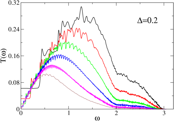
Figure 11: (color online) $2D$ unpinned case with free BC for $\Delta=0.2$.
Plot of the disorder averaged transmission $T(\omega)$ versus $\omega$ for. The curves (from top to bottom) are for $N=16,32,64,128,256,512$ respectively. Note the linear form at small $\omega$.

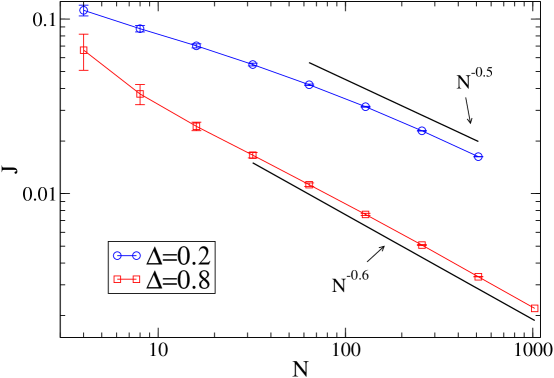
Figure 12: (color online) $2D$ unpinned case with free BC.
Plot of disorder-averaged current $J$ versus system size for two different values of $\Delta$. The error-bars show standard devations due to sample-to-sample fluctuations. Numerical errors are much smaller.

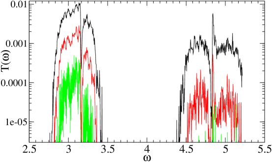
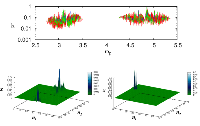
Figure 14: (color online) $2D$ pinned case for $\Delta=0.4$ and $k_{o}=10.0$.
TOP: Plot of the disorder averaged transmission $T(\omega)$ versus $\omega$. The various curves (from top to bottom) correspond to lattices with $N=16,32,64$ respectively. Here we choose $\gamma=\sqrt{10}$.
BOTTOM: Plot of the IPR ($P^{-1}$) as a function of normal mode-frequency $\omega_{p}$. The curves are for $N=16$ (blue), $32$ (green) and $64$ (red). Also shown are two typical normal modes for one small (left) and one large value of $P^{-1}$ for $N=64$.

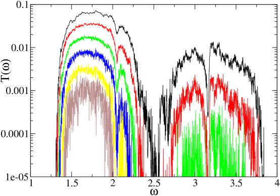
Figure 15: (color online) $2D$ pinned case for $\Delta=0.4$ and $k_{o}=2.0$.
Plot of the disorder averaged transmission $T(\omega)$ versus $\omega$ . The various curves (from top to bottom) are for $N=16,32,64,128,256,512$ respectively. Here we choose $\gamma=\sqrt{2}$.

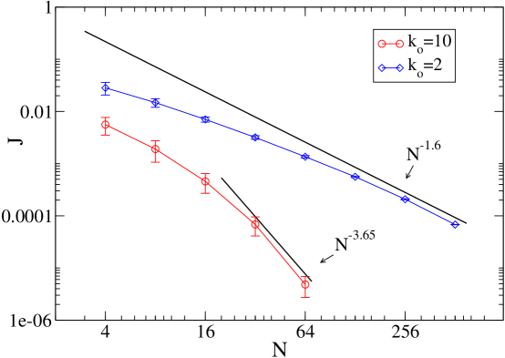
Figure 16: (color online) $2D$ pinned case for $\Delta=0.4$.
Plot of disorder-averaged current $J$ versus system size for two different values of $k_{o}$. Error bars show standard deviation due to disorder and numerical errors are much smaller. Note that the standard deviation do not decrease with system size for higher $k_{o}$.

Figure 17: (color online) $2D$ pinned case for $\Delta=0.4$ and $k_{o}=10.0$.
Plot of disorder-averaged temperature profile $[T_{i}]$ for different system sizes. The plots are from simulations and here we choose $\gamma=\sqrt{10}$.

Figure 18: (color online) $3D$ unpinned case with fixed BC for $\Delta=0.8$.
TOP: Plot of the disorder averaged transmission $T(\omega)$ versus $\omega$. The inset shows the same data multiplied by a factor of $N$.
BOTTOM: Plot of the IPR ($P^{-1}$) and scaled IPR ($N^{3}P^{-1}$) as a function of normal mode-frequency $\omega_{p}$ for a fixed disorder-realization. The curves are for $N=8$ (green) and $16$ (red).

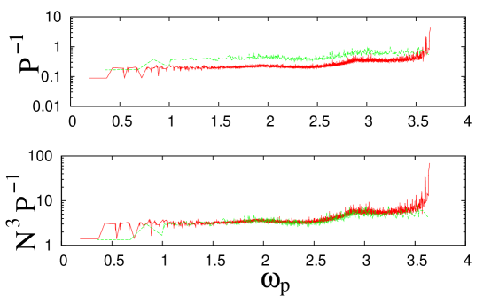
Figure 19: (color online) $3D$ unpinned case with fixed BC for $\Delta=0.2$.
TOP: Plot of the disorder averaged transmission $T(\omega)$ versus $\omega$. The uppermost curve is the transmission curve for the binary mass ordered lattice for $N=16$.
BOTTOM: Plot of IPR ($P^{-1}$) and scaled IPR ($N^{3}P^{-1}$) as a function of normal mode-frequency $\omega_{p}$ for a fixed disorder-realization. The curves are for $N=8$ (green) and $16$ (red).

Figure 20: (color online) $3D$ unpinned case with fixed and free BCs.
Plot of disorder-averaged current $J$ versus system size for two different values of $\Delta$. The data for $\Delta=0.2$ is from simulations. The error-bars show standard deviations due to disorder and numerical errors are smaller.

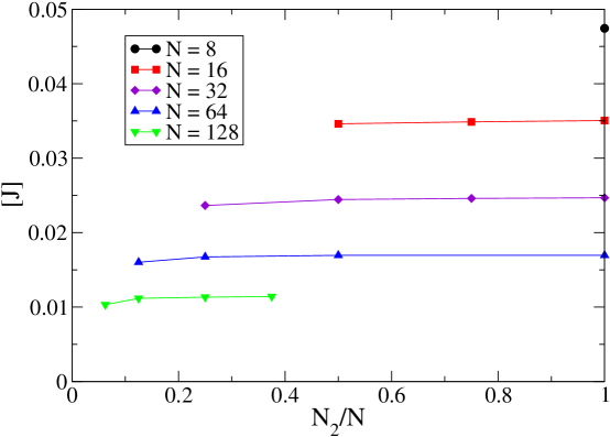
Figure 21: (color online) $3D$ unpinned case with fixed BC for $\Delta=0.2$.
Plot of disorder-averaged current density $J$ (with the definition $J=I/N_{2}^{2}$) versus $N_{2}/N$ for different fixed values of $N$. We see that the 3D limiting value is reached at quite small values of $N_{2}/N$.

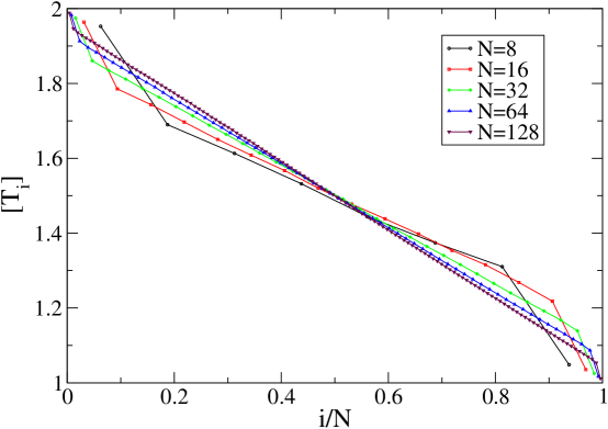
Figure 22: (color online) $3D$ unpinned case with fixed BC for $\Delta=0.2$.
Plot of temperature profile $T_{i}$ in a single disorder realization for different system sizes. The plots are from simulations..

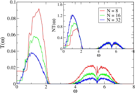
Figure 23: (color online) $3D$ unpinned case with free BC for $\Delta=0.8$.
TOP: Plot of the disorder averaged transmission $T(\omega)$ versus $\omega$. The inset shows the same data multiplied by a factor of $N$.

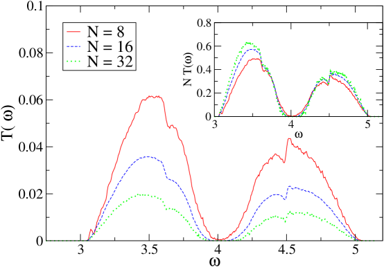
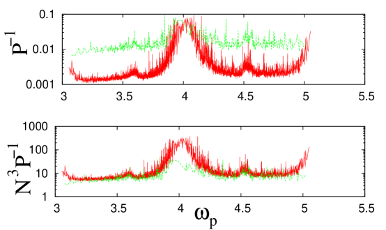
Figure 25: (color online) $3D$ pinned case for $\Delta=0.2$ and $k_{o}=10.0$.
TOP: Plot of the disorder averaged transmission $T(\omega)$ versus $\omega$.
BOTTOM: Plot of the IPR ($P^{-1}$) and scaled IPR ($N^{3}P^{-1}$) as a function of normal mode-frequency $\omega_{p}$. The curves are for $N=8$ (green) and $16$ (red).

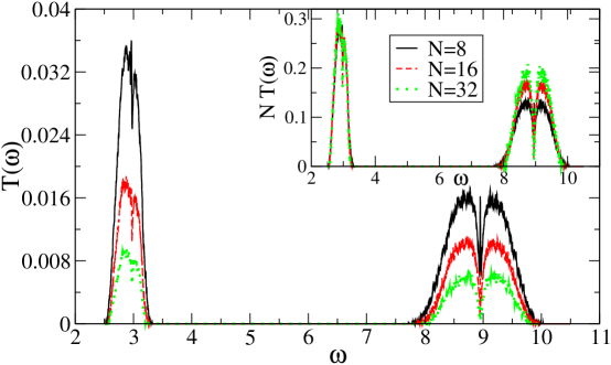
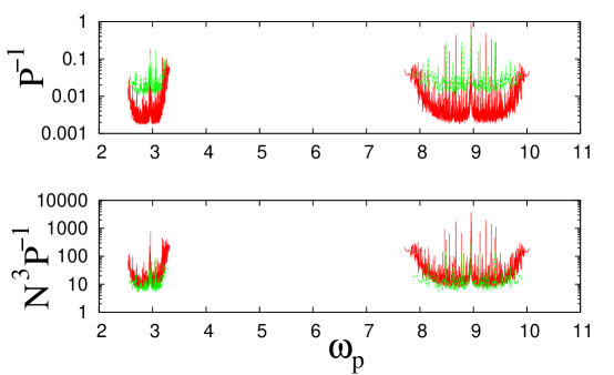
Figure 26: (color online) $3D$ pinned case for $\Delta=0.8$ and $k_{o}=10.0$.
TOP: Plot of the disorder averaged transmission $T(\omega)$ versus $\omega$.
BOTTOM: Plot of the IPR ($P^{-1}$) scaled IPR ($N^{3}P^{-1}$) as a function of normal mode-frequency $\omega_{p}$. The curves are for $N=8$ (green) and $16$ (red).

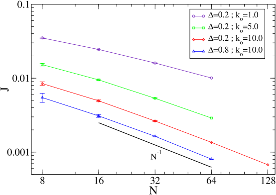
Figure 27: (color online) $3D$ pinned case.
Plot of disorder-averaged current $J$ versus system size for different values of $k_{o}$ and $\Delta$. The data sets for $\Delta=0.2$ for different values of $k_{o}$ are from simulations while the data for $\Delta=0.8$ is from numerics.

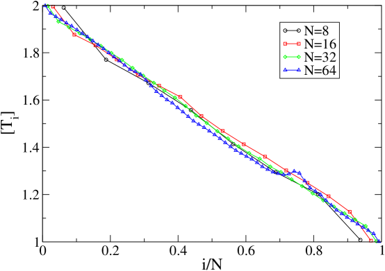
Figure 28: (color online) $3D$ pinned case for $\Delta=0.2$ and $k_{o}=10.0$.
Plot of temperature profile $T_{i}$ in a single disorder realization for different system sizes. The plots are from simulations.

References

- (1) A. Dhar, Adv. Phys., 57, 457 (2008).
- (2) S. Lepri, R. Livi, and A. Politi, Phys. Rep. 377, 1 (2003).
- (3) F. Bonetto, J.L. Lebowitz, and L. Rey-Bellet, in Mathematical Physics 2000, edited by A. Fokas et. al. (Imperial College Press, London, 2000), p. 128.
- (4) C. W. Chang et al. , Phys. Rev. Lett. 101, 075903 (2008).
- (5) D.L. Nika, S. Ghosh, E.P. Pokatilov and A.A. Balandin, Appl. Phys. Lett. 94, 203103 (2009).
- (6) Z. Rieder, J. L. Lebowitz, and E. Lieb, J. Math. Phys. 8, 1073 (1967).
- (7) H. Nakazawa, Progress of Theoretical Physics Supplement 45, 231 (1970).
- (8) P. W. Anderson, Phys. Rev. 109, 1492 (1958).
- (9) N. F. Mott and W. D. Twose, Adv. Phys. 10, 107 (1961).
- (10) R. E. Borland, Proc. R. Soc. London, Ser. A 274, 529 (1963).
- (11) I. Ya. Goldsheid, S. A. Molchanov and L. A. Pastur, Funct. Anal. Appl. 11, 1 (1977).
- (12) P. A. Lee and T. V. Ramakrishnan, Rev. Mod. Phys. 57, 287 (1985).
- (13) S. John, H. Sompolinsky, and M. J. Stephen, Phys. Rev. B 27, 5592 (1983).
- (14) J. Callaway, Phys. Rev. 113, 1046 (1959).
- (15) J. M. Ziman, Principles of the Theory of Solids,(Cambridge University Press, Cambridge, 1972).
- (16) T. Shimada, T. Murakami, S. Yukawa, K. Saito and N. Ito, J. Phys. Soc. Jpn. 69, 3150 (2000).
- (17) H. Shiba and N. Ito, J. Phys. Soc. Jpn. 77, 054006 (2008).
- (18) L. W. Lee and A. Dhar, Phys. Rev. Lett. 95, 094302 (2005).
- (19) P. B. Allen and J. L. Feldman, Phys. Rev. Lett. 62, 645 (1989).
- (20) N. Xu et al., Phys. Rev. Lett. 102, 038001 (2009).
- (21) H. Matsuda and K. Ishii, Prog. Theor. Phys. Suppl. 45, 56 (1970).
- (22) R. J. Rubin and W. L. Greer, J. Math. Phys. 12, 1686 (1971).
- (23) A. Casher and J. L. Lebowitz, J. Math. Phys. 12, 1701 (1971.)
- (24) A. J. O’Connor and J. L. Lebowitz, J. Math. Phys. 15, 692 (1974).
- (25) A. Dhar, Phys. Rev. Lett. 86, 5882 (2001).
- (26) D. Roy and A. Dhar, Phys. Rev. E 78, 051112 (2008).
- (27) A. Dhar and D. Roy, J. Stat. Phys. 125, 801 (2006).
- (28) I. Savic, N. Mingo and D. A. Stewart, Phys. Rev. Lett. 101, 165502 (2008).
- (29) G. Stoltz, M. Lazzeri and F. Mauri, Jn. Phys. Cond. Matt. 21 245302 (2009).
- (30) L. G. C. Rego and G. Kirczenow, Phys. Rev. Lett. 81, 232 (1998).
- (31) M. P. Blencowe, Phys. Rev. B 59, 4992 (1999).
- (32) T. Yamamoto and K. Watanabe, Phys. Rev. Lett. 96, 255503 (2006).
- (33) J. S. Wang, J. Wang and N. Zeng, Phys. Rev. B 74, 033408 (2006).
- (34) M.P. Allen and D.L. Tildesley, Computer Simulation of Liquids (Clarendon Press, Oxford, 1987).
- (35) D. N. Payton and W. M. Visscher, Phys. Rev. 154, 802 (1967).
- (36) P. Dean, Rev. Mod. Phys. 44, 127 (1972).
- (37) A. Dhar and J.L. Lebowitz, Phys. Rev. Lett. 100, 134301 (2008).
- (38) A. Kundu, A. Chaudhuri and A. Dhar, to be published.
- (39) G. Basile, C. Bernardin, S. Olla, Phys. Rev. Lett. 96, 204303 (2006).
- (40) J. Lukkarinen and H. Spohn, Arch. Rat. Mech. Anal. 183, 93 (2007).
- (41) A. MacKinnon and B. Kramer, Z. Phys. B - cond. Matt. 53, 1 (1983).
- (42) J. Hori, Spectral properties of disordered chains and lattices, (Pergamon Press, Oxford, 1968).