2D versus 3D Freezing of a Lennard-Jones Fluid in a Slit Pore: A Molecular Dynamics Study

Abstract

We present a computer simulation study of a (6,12)-Lennard-Jones fluid confined to a slit pore, formed by two uniform planes. These interact via a (3,9)-Lennard-Jones potential with the fluid particles. When the fluid approaches the liquid-to-solid transition we first observe layering parallel to the walls. In order to investigate the nature of the freezing transition we performed a detailed analysis of the bond-orientational order parameter in the layers. We found no signs of hexatic order which would indicate a melting scenario of the Kosterlitz-Thouless type. An analysis of the mean-square displacement shows that the particles can easily move between the layers, making the crystallization a 3d-like process. This is consistent with the fact that we observe a considerable hysteresis in the heating-freezing curves, showing that the crystallization transition proceeds as an activated process.

1 Introduction

Understanding the structure and dynamics of confined fluids is important for processes such as wetting, coating, and nucleation. The properties of a fluid confined in a pore differ significantly from the bulk fluid due to finite size effects, surface forces and reduced dimensionality. In this work we report a study of one of the simplest models that is still capable of reproducing the thermodynamic behavior of classical fluids, the Lennard-Jones (LJ) system. The LJ potential is an important model for exploring the behavior of simple fluids and has been used to study homogeneous vapor-liquid, liquid-liquid and liquid-solid equilibria, melting and freezing. It has also been used as a reference fluid for complex systems like colloidal and polymeric systems.

The vapor-to-liquid transition in confined systems has been studied intensively, and it is well understood (see [1] and references therein). In this article we will discuss the liquid-to-solid transition in a slit pore and the process of the development of the solid phase. In the liquid phase, confinement to a slit induces layering at the walls. One could imagine this effect to facilitate crystallization. And indeed it is known that depending on the strength of the particle-wall interaction different scenarios of freezing exist [2, 3]. If the walls are strongly attractive, crystallization starts from the walls and at a temperature higher than without confinement. If, however, the walls are strongly repulsive, crystallization starts from the bulk at a temperature lower than without confinement. A well-distinguished layer of particles at the wall can also, to some extent, be treated as a 2d system. This raises the question, whether freezing of such a layer proceeds via the Kosterlitz-Thouless-Halperin-Nelson-Young (KTHNY) mechanism [4, 5, 6, 7], meaning that the liquid turns into a crystal going through a hexatic phase [8]. This question has been studied for rather narrow pores (up to 7.5 diameters of a fluid particle). It was found that a hexatic phase exists between liquid and crystal only in the contact layers at the walls [9]. As a consequence, in a pore that can accommodate only a single layer the transition is of the KTHNY type. However, with increasing width the behavior changes to a first order transition [10].

Here we investigate an attractive pore that is significantly wider, namely 20 diameters of a fluid particle. Studying the bond-orientational order parameter within the layers we observe no sign of a hexatic phase. An analysis of the mean-square displacement shows that the particle diffuse between the layers. Hence, the crystallization proceeds as a 3d process, as is also suggested by the noticable hysteresis loop in the heating-freezing curve.

The article is structured as follows. First we describe our simulation method. In section 3. we present the results, followed by a discussion, and in section 4. we conclude with a summary of the presented results.

2 Simulation method

We performed molecular dynamics (MD) simulations in the isothermal ensemble (NVT), i.e. the number of particles N, the volume V and the temperature T were fixed. The system consists of 8000 particles confined between two structureless walls. The particles interact via the LJ-potential

$$u(r)=4\epsilon\left[\left(\frac{\sigma}{r}\right)^{12}-\left(\frac{\sigma}{r}\right)^{6}\right].$$ (1)

The interaction between walls and particles is characterized by a LJ-potential integrated over semi-space:

$$u_{w}(r)=4\epsilon\left[\left(\frac{\sigma}{r}\right)^{9}-\left(\frac{\sigma}{r}\right)^{3}\right].$$ (2)

The particle-particle interaction was cut off at a distance $r_{c}=2.5\sigma$ and the wall-particle interaction at a distance $r_{c}=4.0\sigma$ (the wall-particle potential is wider and deeper then the particle-particle potential). Using for the wall-particles interaction a Steelle potential [11] or just a (4,10)-LJ potential does not influence the results qualitatively. For the following we will use $\epsilon$ as the unit of energy, $\sigma$ as the unit of length and $\tau=\sqrt{1\cdot\sigma^{2}/\epsilon}$ as unit of time (i.e. use the particle mass as the unit of mass); consequently, temperatures are given in multiples of $\epsilon/k_{\mathrm{B}}T$. The simulations were performed in a cubic box with periodic boundary conditions in the x and y direction. The walls were positioned at $z=0$ and $z=L_{z}=20\sigma$. The size of the simulation box was $L_{x}=L_{y}=L_{z}=20\sigma$. We used standard Nosé-Hoover and Langevin thermostats to keep the temperature constant [12, 13, 14]. For the Langevin thermostat, the friction was always chosen as $\Gamma=m\tau^{-1}=1$ [13]. For the Nosé-Hoover thermostat, we set the effective mass $M_{s}=0.5$. We simulated a cooling curve starting out from a random configuration at $T=3.0$ and a melting curve starting out from a face-centered-cubic configuration at $T=1.2$. Far away from the transition, the temperature was changed by $\Delta T=0.1$ from one simulation run to the next, while close to transition we used a smaller increment/decrement, $\Delta T=0.01$.

The simulations were performed with a timestep of $\Delta t=0.005$ and let run for $1.0\times 10^{6}$ MD steps for equilibration and for $2.5\times 10^{5}$ for sampling. In order to compute the mean square displacement of the particles, a smaller timestep $\Delta t=0.002$ was chosen, and to avoid influence of thermostat on the dynamics of the system we switched to the NVE ensemble after equilibration (keeping the total energy of the system $E$ constant). We monitored the temperature, which fluctuated around a mean value practically equal to the temperature T in the NVT ensemble. Pressures were obtained from the virial expansion [15] omitting corrections for the cut-off in the potential. For parts of our simulations the software package ESPResSo version 2.04s was used [16].

3 Results and Discussion

In Figure 1, the pressure-temperature curves for heating and cooling are shown. There is a considerable hysteresis, which indicates that the system has to overcome a free energy barrier when transforming from one phase to the other. Several runs were performed both for heating and for cooling. The cooling lines coincide, whereas the temperature at which the melting process starts fluctuates. In the Figure 1 we show the outer borders of the hysteresis region.

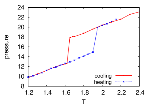
Figure 1: Pressure-Temperature curves for heating and cooling of a LJ-fluid confined between two uniform LJ-walls. The outer borders borders of hysteresis are shown.

As our system has attractive walls, crystallization should start from the walls [2]. This can be clearly seen in the snapshot (Figure 2) that was taken 90 MD steps after equilibration had started. Only another 90 MD steps later the system completely crystallized. One can also see that no crystallization process has started at the right wall yet, demonstrating that this event is an activated process.

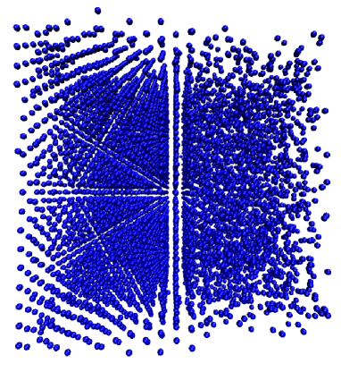
Figure 2: Snapshot of the system in the early stage of crystallization at T=1.60. In this specific example it crystallizes from the left wall. Walls are not represented, but are to the right and to the left of the box. The part on the left is already a crystal while the right side is still disordered.

As it was shown in [2] the width of hysteresis depends on the distance between the layers. If the distance differs considerably from the lattice constant of an ideal LJ crystal ($0.916$), then the hysteresis will be more pronounced. For our system the distance is $0.87$ in the bulk, and correspondingly the hysteresis is quite wide.

In order to investigate the phase transformation process, we now turn to the effects the walls have on the structure of the fluid. Figure 3 shows number density profiles $\varrho(z)$ for $L_{z}=20.0\sigma$ in the liquid and the solid phase. In the liquid phase, the maxima of the peaks follow an exponential law $A\left[\exp(-Bx)+\exp(-(L_{z}-x)B)\right]+\rho_{\mathrm{mid}}$, where $\rho_{\mathrm{mid}}$ is the density in the middle of the box. Figure 4 shows the behavior of the coefficient B with temperature. It can be seen that the values of B decrease more or less linearly at first, i. e. the number of layers increases and they become more pronounced. As soon as we enter the regime of the hysteresis at $T=2.0$, $B$ becomes almost constant (within the error of the simulations). This shows that the structure of the density profile does not change, no new layers appear and the system is trapped in the undercooled state.

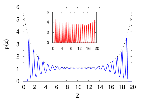
Figure 3: Density profile $\varrho(z)$ of the liquid phase at T=1.70. The heights of the peaks are fitted by an exponential function. The inset shows $\varrho(z)$ for the solid phase at T=1.60.

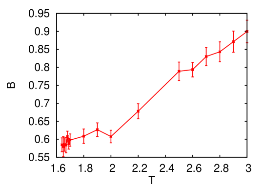
Figure 4: Coefficient $B$ characterizing the exponential decay of density profile. In the hysteresis region $(T<=2.0)$ it almost not changing, i. e. the structure of the density profile stays the same.

As the liquid forms layers, one could assume that the transformation proceeds inside the layers via a KTHNY transition. In order to test this assumption, we now turn to the structure within the layers: To characterize the transitional order in one layer in 2D, we calculate the pair correlation function:

$$g(r)=\varrho^{-2}\langle\sum_{i,i\neq j}\delta(\textbf{r}_{i})\delta(\textbf{r}_{j}-\textbf{r})\rangle$$ (3)

where $\varrho$ is the number density of particles in each layer.

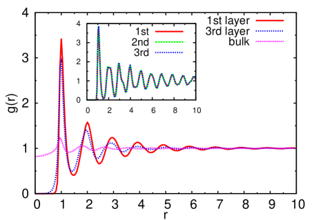
Figure 5: 2D pair correlation function in the first and third layer and the bulk part of the system in the the liquid state at $T=1.65$. The inset shows $g(r)$ for the first three layers at the wall for the solid state at $T=1.60$

In Figure 5 the 2D radial distribution functions for the first and third layer (seen from the wall), the bulk part of the liquid and the first three layers of the solid phase are shown. The structure within the layers of the liquid becomes less pronounced as we move further away from the walls and is barely visible in the center of the box.

Next we consider the bond-orientational order [8]: we define the local bond-orientational order parameter of particle $j$ in layer $m$ at a position $\textbf{x}_{j}$ as

$$\psi^{m}_{6}(\textbf{x}_{j})=\frac{1}{N_{j}}\sum_{k=1}^{N_{j}}e^{i6\theta_{jk}}$$ (4)

where $N_{j}$ is the number of neighbors of particle $j$ within layer $m$, the sum is over the neighbors $k$ of $j$ within $m$, and $\theta_{\textit{jk}}$ is the angle between an arbitrary fixed axis and the line connecting particles j and k. The order of the $m$-th layer $\Psi^{m}_{6}$ is defined as the average over $\psi^{m}_{6}(\textbf{x}_{j})$ for all $N_{m}$ particles within the layer

$$\Psi^{m}_{6}=\frac{1}{N_{m}}|\sum^{N_{m}}_{j=1}\psi^{m}_{6}(\textbf{x}_{j})|\quad.$$ (5)

Figure 6 shows $\Psi^{m}_{6}$ for various temperatures. When approaching the transition, the bond-orientational order close to the wall increases.

The temperature dependence of $\Psi^{1}_{6}$ for the first layer of particles at the wall is shown in Figure 7. It clearly “jumps” i. e. is discontinuous at the transition.

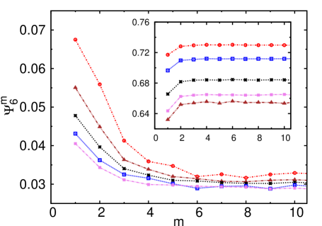
Figure 6: 2D bond-orientation order parameter $\Psi^{m}_{6}$ for liquid states depending on the layer $m$ for temperatures 1.70, 1.80, 2.00, 2.20, 2.40 (from top to bottom). The inset shows $\Psi^{m}_{6}$ for solid states for temperatures 0.80, 1.00, 1.30, 1.50, 1.60 (from top to bottom).

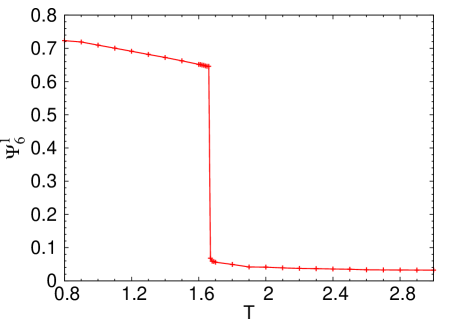
Figure 7: 2D bond-orientation order parameter $\Psi^{1}_{6}$ of the first layer from the wall as a function of the temperature.

If the crystallization proceeded purely within the two-dimensional layers, one would observe a hexatic phase, which is characterized by a power-law decay of the correlation of the bond-orientational order

$$g_{6}(r)=\langle\psi^{*}_{6}(\textbf{x}^{{}^{\prime}})\psi_{6}(\textbf{x}^{{}^{\prime}}-\textbf{x})\rangle\quad,$$ (6)

where the average is taken over all particles within a layer whose positions x are a distance $r$ apart.

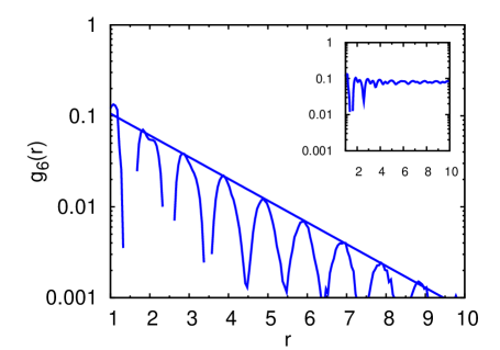
Figure 8: Bond-orientational correlation function for the liquid state just before freezing at $T=1.67$ for the layer closest to the wall. The solid line is the result of an exponential fit. There is no signature of a hexatic phase. The inset shows $g_{6}$ for the crystallin state at the next available lower temperature $T=1.66$, right after the transition.

Figure 8 shows $g_{6}(r)$ for the first layer at $T=1.67$ and $T=1.66$. The system jumps from the 2d-liquid phase into the 2d-solid without visiting a hexatic phase first. Hence the crystallization process is not of the KTHNY-kind.

To find out why the crystallization process is 3d-like despite the layering, we now consider the particles’ dynamics. One of the obvious characterictics is to estimate how long particles on average stay in the layer closest to the wall. The easiest way to estimate this is to calculate how many particles of those which were in the layer at time 0 remained there at the time $t$. From Figure 9 we can see that the ratio of particles that remain in the layer decreases exponentially with time. Fitting it with $\exp(-t/\tau)$ we obtain the average lifetime $\tau$ of a particle in the layer (Figure 10). It increases linearly with the decrease of temperature and is then fluctuating around the mean value in the hysteresis region. As we observed already for the density, the behavior of the system in the hysteresis region does not change much during cooling.

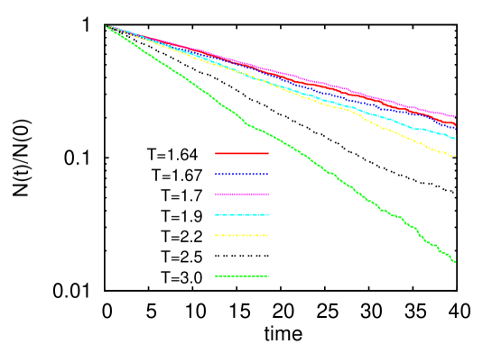
Figure 9: Ratio of particles in the layer closest to the wall that stayed there from time $0$ ($N(0)$) until time $t$ ($N(t)$) at different temperatures above the phase transition.

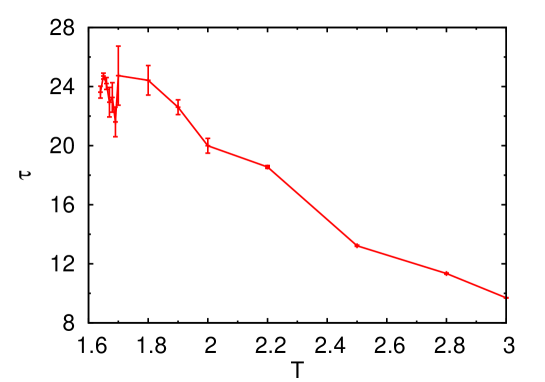
Figure 10: Average lifetime of particles in the outmost layer as a function of temperature. In the hysteresis region the lifetime does not change significantly.

To characterize the mobility of the particles we calculated the mean square displacement (MSD). As the system forms layers, we calculate the MSD parallel and perpendicular to the wall separately. Looking at the plane parallel to the wall (Figure 11) while approaching crystallization, we observe that the particles in the layer closest to the wall are a little faster than the particles in the bulk, despite the fact that the crystallization typically starts from here. We take this as another hint that the crystallization proceeds as a 3d-process, and does not first start within the layer closest to the wall. The behavior of the particles does not change significantly on approach of the crystallization as they enter the metastable region.

The mean square displacement measured perpendicular to the wall (Figure 11) shows that after the ballistic regime for a while particles are trapped in the layer and then start leaving it. It is not meaningful to calculate the diffusion coefficient in our system, because the particles do not stay long enough in a layer for the MSD to enter the linear regime.

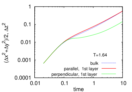
Figure 11: Mean square displacement for $T=1.64$. The MSD parallel to the wall is almost identical in the layer and in the bulk with the particles in the layer even being slightly faster. The MSD perpendicular to the wall show a clear trapping effect.

4 Conclusions

We reported on a molecular dynamics study of the liquid-to-solid transformation of a LJ fluid in a wide slit pore. Although the confinement induces layering in the liquid phase close to the walls, we do not find a successive, layerwise crystallization. Crystallization is still a 3d process, and, in particular, no hexatic phase was observed in the layers closest to the wall, excluding the possibility of a 2D KTHNY-like crystallization within the layers; in fact, the mobility of particles in the layers is higher than their mobility in the bulk. Nevertheless, we find that crystallization in the system practically always starts from the walls, i. e., the walls facilitate crystallization. And although crystallization is an activated process similar to 3d crystallization, we observe a smaller hysteresis, indicating a reduced nucleation barrier as compared to bulk crystallization.

Alltogether, our simulations suggest that the nucleation of the LJ fluid close to a planar wall does not significantly differ from the nucleation in the bulk, although with a smaller nucleation barrier. This can however be easily understood as an effect of the strongly increased density in the layers close to the confinement.

References

- [1] Lev D Gelb, K E Gubbins, R Radhakrishnan, and M Sliwinska-Bartkowiak. Phase separation in confined systems. Rep. Progr. Phys., 62(12):1573–1659, 1999.
- [2] M. Miyahara and K. E. Gubbins. Freezing/melting phenomena for lennard-jones methane in slit pores: A monte carlo study. J. Chem. Phys., 106:2865–2880, 1997.
- [3] C Alba-Simionesco, B Coasne, G Dosseh, G Dudziak, K E Gubbins, R Radhakrishnan, and M Sliwinska-Bartkowiak. Effects of confinement on freezing and melting. J. Phys.: Condens. Matter, 18:R15–R68, 2006.
- [4] J M Kosterlitz and D J Thouless. Ordering, metastability and phase transitions in two-dimensional systems. J. Phys. C: Solid State Phys., 6(7):1181–1203, 1973.
- [5] B. I. Halperin and David R. Nelson. Theory of two-dimensional melting. Phys. Rev. Lett., 41(2):121–124, Jul 1978.
- [6] David R. Nelson and B. I. Halperin. Dislocation-mediated melting in two dimensions. Phys. Rev. B, 19(5):2457–2484, Mar 1979.
- [7] A. P. Young. Melting and the vector coulomb gas in two dimensions. Phys. Rev. B, 19(4):1855–1866, Feb 1979.
- [8] K. J. Strandburg. Two-dimensional melting. Rev. Mod. Phys., 60:161–207, 1988.
- [9] R. Radhakrishnan, K. E. Gubbins, and M. Sliwinska-Bartkowiak. Global phase diagrams for freezing in porous media. J. Chem. Phys., 116(3):1147–1155, 2002.
- [10] R. Radhakrishnan, K. E. Gubbins, and M. Sliwinska-Bartkowiak. Existence of a hexatic phase in porous media. Phys. Rev. Lett., 89(7):076101, Jul 2002.
- [11] W. A. Steele. The physical interaction of gases with crystalline: I. gas-solid energies and properties of isolated adsorbed atoms. Surf. Sci., 36:317–352, 1973.
- [12] D. C. Rapaport. The Art of Molecular Dynamics Simulation. Cambridge University Press, 2004.
- [13] M. P. Allen and D. J. Tildesley. Computer Simulation of Liquids. Clarendon, Oxford, 1987.
- [14] D. Frenkel and B. Smit. Understanding Molecular Simulation. Academic Press, 2002.
- [15] J. P. Hansen and I. R. McDonald. Theory of Simple Liquids. Academic Press, London, 1986.
- [16] H. J. Limbach, A. Arnold, B. A. Mann, and C. Holm. ESPResSo – an extensible simulation package for research on soft matter systems. Comp. Phys. Comm., 174(9):704–727, May 2006.