Suzaku View of the Swift/BAT Active Galactic Nuclei (I):
Spectral Analysis of Six AGNs
and Evidence for Two Types of Obscured Population

Abstract

We present a systematic spectral analysis with Suzaku of six AGNs detected in the Swift/BAT hard X-ray (15–200 keV) survey, Swift J0138.6–4001, J0255.2–0011, J0350.1–5019, J0505.7–2348, J0601.9–8636, and J1628.1–5145. This is considered to be a representative sample of new AGNs without X-ray spectral information before the BAT survey. We find that the 0.5–200 keV spectra of these sources can be uniformly fit with a base model consisting of heavily absorbed (log $N_{\rm H}>$23.5 cm^-2) transmitted components, scattered lights, a reflection component, and an iron-K emission line. There are two distinct groups, three “new type” AGNs (including the two sources reported by Ueda et al. 2007) with an extremely small scattered fraction ($f_{\rm scat}<0.5\%$) and strong reflection component ($R=\Omega/2\pi\gtrsim 0.8$ where $\Omega$ is the solid angle of the reflector), and three “classical type” ones with $f_{\rm scat}>0.5\%$ and $R\lesssim 0.8$. The spectral parameters suggest that the new type has an optically thick torus for Thomson scattering ($N_{\rm H}\sim 10^{25}$ cm^-2) with a small opening angle $\theta\sim 20^{\circ}$ viewed in a rather face-on geometry, while the classical type has a thin torus ($N_{\rm H}\sim 10^{23-24}$ cm^-2) with $\theta\gtrsim 30^{\circ}$. We infer that a significant number of new type AGNs with an edge-on view is missing in the current all-sky hard X-ray surveys.

1. Introduction

The growth history of supermassive black holes (SMBHs) in galactic centers is a key question for understanding cosmic history. This can be traced by observations of Active Galactic Nuclei (AGNs), where mass accretion onto SMBHs is taking place. Many observations indicate that obscured AGNs are the major AGN population both in the local universe and at intermediate-to-high redshifts (see e.g., Hasinger, 2008). In fact, much of the SMBH growth is theoretically expected to happen during an obscured phase in the evolution of AGNs (e.g., Hopkins et al., 2006). Thus, detecting all the obscured AGNs in the universe and revealing their nature is a fundamental issue to be addressed by modern astrophysics. Our knowledge of this population is still quite limited even in the local universe, due the difficulty of detecting highly absorbed objects in most wavelength bands.

Table 1List of Targets

SWIFT	Optical/IR Identification	R.A. (J2000)	Dec. (J2000)	Redshift	Classification
J0138.6–4001	ESO 297–G018	01 38 37.16	-40 00 41.1	0.0252	Seyfert 2
J0255.2–0011	NGC 1142	02 55 12.196	-00 11 0.81	0.0288	Seyfert 2
J0350.1–5019	2MASX J03502377–5018354	03 50 23.77	-50 18 35.7	0.036	Galaxy
J0505.7–2348	2MASX J05054575–2351139	05 05 45.73	-23 51 14.0	0.0350	Seyfert 2
J0601.9–8636	ESO 005–G004	06 05 41.63	-86 37 54.7	0.0062	Galaxy
J1628.1$+$5145	Mrk 1498	16 28 4.06	+51 46 31.4	0.0547	Seyfert 1.9

Note. — The position, redshift, and classification for each source is taken from the NASA/IPAC Extragalactic Database.

Obscured AGNs, often referred as type 2 AGNs, are characterized by heavily absorbed X-ray spectra and/or by the absence of broad emission lines in the optical spectra. The unified model of AGNs attributes these differences to the blockage of the line of sight by a dusty torus. Recent X-ray and IR observations have revealed populations of AGNs without any signature of AGNs in the optical band (e.g., Maiolino et al., 2003). This fact implies that AGN surveys relying on optical emission signatures (such as the [O III] $\lambda 5007$ line) may be incomplete.

Sensitive hard X-ray observations above 10 keV provide us with the least biased AGN samples in the local universe, due to the strong penetrating power against photo-electric absorption, except for heavily Compton thick (column density of log $N_{\rm H}$ $\gtrsim$ 24.5 cm^-2) objects. Recent all sky hard X-ray surveys performed with Swift/BAT (Tueller et al., 2008) and INTEGRAL (Bassani et al., 2006; Krivonos et al., 2007) have started to detect many local AGNs with about 10 times better sensitivity than that of previous missions in this energy band. They have shown that roughly half of all local AGN are indeed obscured AGNs. These hard X-ray samples contain a number of new AGNs, for which detailed follow-up studies have not been done yet. Some of these sources objects were not recognized to be AGNs previously even though there were optical imaging and spectroscopy data available.

Our team has started to make follow-up observations of selected Swift/BAT AGNs with the Suzaku satellite to obtain the best quality broad band high energy data. The major purposes are (1) to discover new populations of AGNs, (2) to measure their spectral properties, which make it possible to construct the $N_{\rm H}$ distribution of a complete Swift/BAT sample, and (3) to accurately constrain the strength of the reflection component, which is an important yet uncertain parameter in population synthesis models of the X-ray background in explaining its broad-band shape (Ueda et al., 2003; Gilli et al., 2007). In particular, the simultaneous coverage over the 0.2–70 keV band with Suzaku is crucial to discriminate degeneracy of spectral models under possible time variability and to determine the amounts of scattered and reflected components, key information to constrain the geometry of surrounding matter around the nucleus.

The first results obtained from the Suzaku follow-up of two Swift/BAT AGNs led to the discovery of a new type of deeply buried AGNs (Ueda et al., 2007). Here we present the results of a detailed analysis of six Swift/BAT AGNs, including the two sources (Swift J0138.6–4001 and Swift J0601.9–8636) already reported there. This paper constitutes the first one in the series of papers to be published on Suzaku-Swift AGNs, followed by the second paper by Winter et al. (in preparation). § 2 summarizes the sample and observations. In § 3, we mainly present the results of detailed spectral analysis with Suzaku. Discussion is given in § 4. We adopt the cosmological parameters ($H_{0}$, $\Omega_{\rm m}$, $\Omega_{\lambda}$) = (70 km s^-1 Mpc^-1, 0.3, 0.7) throughout the paper.

2. Observations

Table 2Observation Log

SWIFT	Start Time (UT)	End Time	Exposure (XIS)	Exposure (HXD/PIN)	SCI
J0138.6–4001	2006 Jun 04 18:13	Jun 05 05:00	21.2 ks	16.5 ks	Off
J0255.2–0011	2007 Jan 23 14:54	Jan 26 05:30	101.6 ks	80.6 ks	On
J0350.1–5019	2006 Nov 23 02:07	Nov 23 13:33	19.3 ks	15.7 ks	On
J0505.7–2348	2006 Apr 01 22:12	Apr 04 02:55	78.6 ks	50.3 ks	Off
J0601.9–8636	2006 Apr 13 16:24	Apr 14 01:52	19.8 ks	15.7 ks	Off
J1628.1$+$5145	2006 Apr 15 18:49	Apr 16 09:22	23.6 ks	19.5 ks	Off

Figure 1.— The background subtracted light curves of XIS in the 2–10 keV band during the Suzaku observations. One bin corresponds to 96 minutes. The data from the XIS-0 and XIS-2 are summed for Swift J0255.2–0011 and Swift J0350.1–5019, while those from XIS-0, XIS-2, and XIS-3 are summed for the rest. The numbers listed in each panel represent the value of reduced $\chi^{2}$ with the degree of freedom for the constant flux hypothesis.

Table 3Cutoff Energies ($E_{\rm{cut}}$) determined by the BAT spectra

$\Omega/2\pi$	SWIFT J0138.6–4001	J0255.2–0011	J0350.1–5019	J0505.7–2348	J0601.9–8636	J1628.1$+$5145
$0$	$>317$	$>289$	$>106$	$>318$	$>116$	$>99$
$\chi^{2}/\rm{d.o.f.}$	$1.58/2$	$4.57/6$	$1.16/6$	$13.58/6$	$4.96/2$	$2.38/6$
$2$	$329$ ($>91$)	$>253$	$>95$	$>306$	$>82$	$>87$
$\chi^{2}/\rm{d.o.f.}$	$1.05/2$	$5.21/6$	$2.40/6$	$15.24/6$	$3.37/2$	$4.61/6$

Note. — The unit of $E_{\rm{cut}}$ is keV.

Figure 2.— The background subtracted light curves of HXD/PIN in the 15–40 keV band during the Suzaku observations. One bin corresponds to 96 minutes. The numbers listed in each panel represent the value of reduced $\chi^{2}$ with the degree of freedom for the constant flux hypothesis.

We observed six Swift/BAT AGNs with Suzaku between 2006 April and 2007 January in the AO-1 phase. The targets are Swift J0138.6–4001, J0255.2–0011, J0350.1–5019, J0505.7–2348, J0601.9–8636, and J1628.1–5145, whose identification in the optical or infrared band is ESO 297–G018, NGC 1142, 2MASX J03502377–5018354, 2MASX J05054575–2351139, ESO 005–G004, and Mrk 1498, respectively (Tueller et al., 2008). The basic information of our targets is summarized in Table 1. 2MASX J03502377–5018354 and ESO 005–G004 had not been identified as active galaxies in the optical band, and revealed to contain an AGN for the first time with the detection of hard X-rays by the BAT. The sources were selected as the Suzaku targets because at the time of our proposals these “new” Swift AGNs had no spectral information available below 10 keV. Recently short follow-up observations of these targets have been carried out with XMM-Newton or the X-Ray Telescope (XRT) onboard Swift (Winter et al., 2008a).

Suzaku, the fifth Japanese X-ray satellite (Mitsuda et al., 2007), carries four X-ray CCD cameras called the X-ray Imaging Spectrometer (XIS-0, XIS-1, XIS-2, and XIS-3; Koyama et al. 2007) as focal plane imager of four X-ray telescopes, and a non-imaging instrument called the Hard X-ray Detector (HXD; Takahashi et al. 2007) consisting of Si PIN photo-diodes and GSO scintillation counters. XIS-0, XIS-2, and XIS-3 are front-side illuminated CCDs (FI-XISs), while XIS-1 is the back-side illuminated one (BI-XIS).

In this paper, we analyze the data of the XISs and the HXD/PIN (HXD nominal position), which covers the energy band of 0.2–12 keV and 10–60 keV, respectively, since the fluxes of our targets above 50 keV are too faint to be detected with the HXD/GSO. Table 2 shows the log of the observations. The net exposure of Swift J0255.2–0011 and Swift J0505.7–2348 is about 100 ks and 80 ks, respectively, while that for the rest 4 targets is 20 ks each. Because XIS-2 became unoperatable on 2007 November 7 (Dotani et al., 2007), no XIS-2 data are available for Swift J0255.2–0011 and Swift J0350.1–5019. For the observations of Swift J0255.2–0011 and Swift J0350.1–5019, we applied spaced-row charge injection (SCI) for the XIS data to improve the energy resolution (Nakajima et al., 2008). In the spectral analysis, we also utilize the BAT spectra covering the 15–200 keV band, integrated for the first 9 months for Swift J0138.6–4001 and Swift J0601.9–8636, and for 22 months for the rest of targets.

3. Analysis and Results

We analyze the Suzaku data using HEAsoft version 6.3.2 from the data products version 2.0 distributed by the Suzaku pipeline processing team. In extraction of the light curves and spectra, we set the source region as a circle around the detected position with a radius of 1.5–2 arcmin, depending on the flux. For the XIS data, the background was taken from a source-free region in the field of view with an approximately same offset angle from the optical axis as the source. For the HXD/PIN data, we use the so-called “tuned” background model provided by the HXD team. Its systematic errors are estimated to be $\simeq 1.3\%$ at a $1\sigma$ confidence level in the 15–40 keV band for a 10 ks exposure (Mizuno et al., 2008). As our exposures are $\approx$20 ks or larger, we expect that the error is even smaller than this value.

3.1. Light Curves

Figures 1 and 2 show the background-subtract light curves of our targets obtained with the XIS and HXD in the 2–10 keV and 15–40 keV band, respectively. To minimize any systematic uncertainties caused by the orbital change of the satellite, we merge data taken during one orbit (96 minutes) into one bin. Then, to check if there is any significant time variability during the observations, we perform a simple $\chi^{2}$ test to each light curve assuming a null hypothesis of a constant flux. The resultant reduced $\chi^{2}$ value and the degree of freedom are shown in each panel. We detect no significant time variability on a time scale of hours for all the targets in both energy bands. Thus, we analyze the spectra of all the targets averaged over the whole observation epoch.

3.2. BAT Spectra

Before performing the spectral fit to the Suzaku data, we firstly analyze only the BAT spectra in the 15–200 keV band to constrain the high energy cutoff in the continuum. It is known that the incident photon spectra of Seyfert galaxies are well approximated by a power law with an exponential cutoff (cutoff power law model), represented as $AE^{-\Gamma}\exp\{-E/E_{\rm cut}\}$, where $A$, $\Gamma$, $E_{\rm cut}$ is the normalization at 1 keV, photon index, cutoff energy, respectively. Here we utilize the pexrav code by Magdziarz & Zdziarski (1995) to take into account possible contribution of the Compton reflection component from optically thick, cold matter. The relative intensity of the reflection component to that of the incident cutoff power law component is defined as $R\equiv\Omega/2\pi$, where $\Omega$ is the solid angle of the reflector ($R=1$ corresponds to the reflection from a semi-infinite plane).

In this stage, we assume $R$ = 0 or 2 as the two extreme cases just to evaluate the effects of the reflection. The inclination angle is fixed at $60^{\circ}$. To avoid strong coupling between the power law slope and and cutoff energy, we fix the photon index at 1.9, which is a canonical value for AGNs. Table 3 summarizes the fitting results of the cutoff energy for each target. While it is difficult to constrain its upper limit due to the limited band coverage of the BAT, we find the cutoff energy must be above $\approx$100 keV in most cases. Considering this limitation, we fix $E_{\rm cut}$ at 300 keV in all subsequent analysis. Impacts by adopting a lower value of $E_{\rm{cut}}$ in the spectral fitting are discussed in §3.5.

3.3. Spectral Models

We consider three basic models in the spectral analysis uniformly for all the six targets. Our policy is to start with the simplest model for each target; if we find that the fit with a simple model does not give a physically self-consistent picture and/or that the fit is significantly improved by introducing additional parameters, then we adopt more complicated models. In all the cases, we assume a power law with an exponential cutoff fixed at 300 keV for the incident continuum, as explained in the previous subsection. The Galactic absorption, $N_{\rm{H}}^{\rm{Gal}}$, is always included in the model (even if not explicitly mentioned below) by assuming the hydrogen column density from the H I map of Kalberla et al. (2005), available with the nh program in the HEAsoft package. For absorption, we adopt the photo-electric absorption cross section by Balucinska-Church & McCammon (1992) (“bcmc”) and use the phabs or zphabs model in XSPEC. Solar abundances by Anders & Grevesse (1989) are assumed throughout the analysis.

The first (simplest) model, designated as Model A, consists of (i) a transmitted component (a cut-off power law absorbed by cold matter), (ii) a scattered component (a cut-off power law without absorption), and (iii) an iron-K emission line (a gaussian), represented as zphabs*zhighect*zpowerlw + const*zhighect*zpowerlw + zgauss in the XSPEC terminology. According to the unified scheme, in type 2 AGNs, the incident power law from the nucleus will be absorbed by a dusty torus around the SMBH, while the nuclear emission is partially scattered into the line-of-sight by ionized gas around the torus. For simplicity, we assume that the scattered component has the same shape of the incident power law with a fraction of $f_{\rm scat}$ as first-order approximation, although, in reality, it often contains a number of recombination lines produced by a photo-ionized plasma (e.g., Sako et al., 2000) unless the scatterer is fully ionized. As a result of reprocessing by cold matter in the surrounding environment (such as a torus, an ionized gas, and an accretion disk), an iron-K emission will be produced at the rest-frame 6.4 keV. Since a line from the torus should not resolved by the energy resolution of the XIS, we fix the $1\sigma$ line width of the iron-K line at the averaged value of the (apparent) line width of the ${}^{55}\rm{Fe}$ calibration source at 5.9 keV: 0.3 eV, 38 eV, 30 eV, 0.8 eV, 1.7 eV and 3.2 eV for Swift J0138.6–4001, J0255.2–0011, J0350.1–5019, J0505.7–2348, J0601.9–8636, and J1628.1–5145, respectively, to take into account a possible systematic error in the energy response .

In the second model, Model B, we consider an additional contribution of an absorbed Compton reflection component from optically thick matter. This emission is expected from the inner wall of an (optically thick) torus and/or the accretion disk, irradiated by the incident continuum. Model B is expressed as zphabs*zhighect*zpowerlw + const*zhighect*zpowerlw + zgauss + zphabs*pexrav in the XSPEC terminology, where the last term represents the reflection component (not including the direct one). In the pexrav model, we make the solid angle $\Omega$ of the reflector seen from the nucleus as a free parameter, and fix the inclination angle and the cutoff energy at $60^{\circ}$ and $300\ \rm{keV}$, respectively. The photon index and normalization of the power law are linked to those of the transmitted component. The absorption to the reflection component is set to be independent of that for the transmitted one, by considering a different geometry of the emission region. To check the physical validity of Model B, we examine the equivalent width (E.W.) of the iron-K emission line with respect to the reflection component, $\rm{E.W.}^{\rm{refl}}$, obtained from the fit. Theoretically, it is expected to be 1–2 keV (Matt et al., 1991). This value, however, tightly depends on the geometries of the torus and the accretion disk. Thus, we regard the result of Model B as valid only if $\rm{E.W.}^{\rm{refl}}=0.5-2\ \rm{keV}$ but discard it otherwise.

We finally consider the third model (Model C), where we assume two different absorptions with different covering factors for the transmitted component. This reduces the contribution of a less absorbed reflection component compared with the case of a single absorption as assumed in Model B. In fact, simulations show that the absorber in the torus can be patchy (Wada & Norman, 2002), resulting in a time-averaged spectrum that is better modeled by multiple absorptions to the transmitted continuum rather than by a single absorber. In the XSPEC terminology, Model C is expressed as zphabs*zpcfabs*zhighect*zpowerlw + const*zhighect*zpowerlw + zgauss + zphabs*pexrav, where the multiple terms of the first component (absorbed, partial covering model) represents the two different absorptions.

To summarize, we can write the three models of the photon spectrum $F\left(E\right)$ without the Galactic absorption as follows:

$$F\left(E\right)=f_{\rm c}\exp\left\{-N_{\rm H}^{\rm a}\sigma\left(E\right)\right\}I\left(E\right)+\left(1-f_{\rm c}\right)\exp\left\{-N_{\rm H}^{\rm b}\sigma\left(E\right)\right\}I\left(E\right)$$

$$+f_{\rm{scat}}I\left(E\right)+G\left(E\right)+\exp\left\{-N_{\rm{H}}^{\rm{refl}}\sigma\left(E\right)\right\}C\left(E\right)+S\left(E\right),$$ (1)

where $f_{\rm c}$ is the fraction of the more heavily absorbed component ($f_{\rm c}=1$ in Models A and B), $N_{\rm H}^{\rm a}$ and $N_{\rm H}^{\rm b}$ are the absorption column densities for the transmitted component ($N_{\rm H}^{\rm b}=0$ in Models A and B), $\sigma\left(E\right)$ is the cross section of photoelectric absorption, $I\left(E\right)\equiv AE^{-\Gamma}\exp\{-E/E_{\rm cut}\}$ is the intrinsic cutoff power law component, $f_{\rm{scat}}$ is the scattered fraction, $G\left(E\right)$ is a gaussian representing the iron-K emission line, $C\left(E\right)$ is the Compton reflection component ($C\left(E\right)=0$ in Model A), and $S\left(E\right)$ represents additional soft components (see below).

3.4. Fitting Results

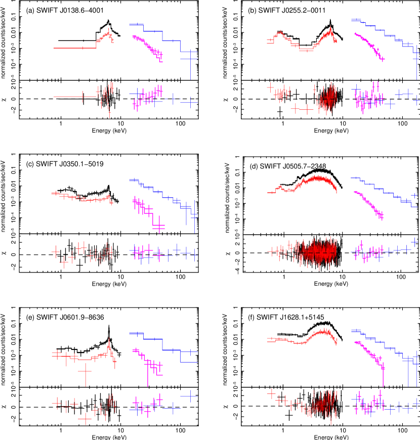
Figure 3.— The observed spectra of the 6 targets. The black, red, magenta and blue crosses represent the data of the FI-XIS, BI-XIS, HXD/PIN, and BAT, respectively, showing their 1$\sigma$ errors in vertical direction. The spectra of the XIS and PIN are folded with the detector response in units of counts s^-1 keV^-1, while those of the BAT is corrected for the detector area and have units of photons cm^-2 ks^-1 keV^-1. The best-fit models are plotted by lines, and the residuals in units of $\chi$ are shown in the lower panels.

Using the three models described in the previous subsection, we perform spectral fit simultaneously to the spectra of the FI-XISs (those of 2 or 3 XISs are summed), the BI-XIS, and the HXD/PIN. Based on the fitting results, we chose the best model in the following manner. (1) First, if Models B is found to significantly improve the fit from Model A by performing an F-test, we tentatively adopt Model B as a better model, otherwise Model A. (2) Then, if Model B is found to be physically not self-consistent in terms of the E.W. of the iron-K line as explained in the previous subsection, or if Model C significantly improves the fit compared with Model A, we adopt Model C as the best model.

After finding the best one among the three models, we finally include the Swift/BAT spectrum to the Suzaku data to constrain the photon index most tightly, assuming that the spectral variability is negligible between the observation epoch of Suzaku and that of Swift. In the fit, we fix the relative normalization between the FI-XISs and the PIN at 1.1 based on the calibration of Crab Nebula (Ishida et al., 2007), while those of the BI-XIS and the BAT against FI-XISs are treated as free parameters, considering the calibration uncertainty and time variability (in flux), respectively. The detailed results of spectral fit for each source is summarized below.

Swift J0138.6–4001

We adopt Model B as the most appropriate model of Swift J0138.6–4001. We obtain $(\chi^{2},\nu)$ = $(101.14,\ 96)$ with Model A and $(92.52,\ 94)$ with Model B, where $\nu$ is the degree of freedom. Thus, the improvement of the fit by adding a reflection component is found to be significant at $>$90% confidence level by an $F$-test, which gives an $F$-value of 4.38 for the degrees of freedom of $(2,\ 94)$. Since the E.W. of the iron-K line with respect to the reflection component is found to be $\rm{E.W.}^{\rm{refl}}>$ 0.5 keV, the model is physically self-consistent. Here we allow the absorption to the reflection component $N_{\rm{H}}^{\rm{refl}}$ to be a free parameter, unlike the case in Ueda et al. (2007), where it is linked to that for the transmitted component. The basic results are essentially unchanged, however.

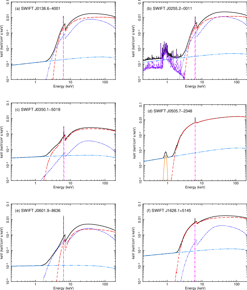
Figure 4.— The best fit spectral model of the 6 targets in units of $EF_{E}$ (where $E$ is the energy and $F_{E}$ is the photon spectrum). The black, dashed red, dotted blue, dot-dot-dashed cyan, dot-dashed magenta curves correspond to the total, transmitted one, reflection component , scattered component, and iron-K emission line, respectively. The purple dashed model in Swift J0255.2–0011 represents the emission from an optically-thin thermal plasma, and the orange one in Swift J0505.7–2348 the Ne emission lines from a photo-ionized plasma (see text).

Swift J0255.2–0011

We adopt Model B with a apec plasma model for Swift J0255.2–0011. Models A and B yield $(\chi^{2},\ \nu)$ = $(596.85,\ 304)$ and $(500.75,\ 302)$, respectively, suggesting the presence of a significant amount of a reflection component. We find $\rm{E.W.}^{\rm{refl}}=0.81^{+0.07}_{-0.09}$ keV with Model B, which is physically consistent. We also confirm that applying Model C does not improve the fit significantly, yielding $f_{c}=1.0$ (i.e., multiple absorbers for the transmitted component are not required when we consider a reflection component). As positive residuals remain in the energy band below 1 keV, we add the apec model in XSPEC, an emission model from an optically-thin thermal plasma with Solar abundances, over Model B. It greatly improve the fit, giving $(\chi^{2},\nu)=(330.38,\ 300)$. The temperature of the plasma is found to be $kT=0.74^{+0.03}_{-0.10}\ \rm{keV}$ with an emission measure of $n^{2}V\approx 5\times 10^{63}\ \rm{cm}^{-3}$. This temperature is similar to those found in many Seyfert 2 galaxies (Turner et al., 1997).

Swift J0350.1–5019

Model C is adopted for Swift J0350.1–5019 since we find $\rm{E.W.}^{\rm{refl}}$ $<0.1\ \rm{keV}$ . We obtain $(\chi^{2},\nu)$ = $(34.93,\ 36)$ with Model A, and $(28.24,\ 35)$ with Model B. Here, we link the absorption to the reflection component and that to the transmitted one, as having the former as a free parameter does not help improving the fit. Model C gives $(\chi^{2},\nu)$ = $(28.24,\ 35)$ and $\rm{E.W.}^{\rm{refl}}=2.8^{+1.4}_{-1.3}$ keV, which is now physically consistent.

Swift J0505.7–2348

We adopt Model C with a line feature at $\approx$0.9 keV as the best description for Swift J0505.7–2348. We find very little reflection component in the spectra of Swift J0505.7–2348; Models A and B give a very similar $\chi^{2}$ value of 671.3 for a degree of freedom of 602 and 600, respectively, with no improvement of the fit by Model B. In fact, we obtain a tight upper limit for the reflection component of $R<0.11$ (90% confidence level) from the fit with Model B. Thus, we apply Model C (here $N_{\rm{H}}^{\rm{refl}}$ is tied to $N_{\rm{H}}^{\rm{b}}$ since $R\simeq 0$). This model yields $(\chi^{2},\ \nu)=(636.11,\ 598)$, which is significantly better than Model A (or B). Furthermore, positive residuals remain in the 0.7–1 keV band, centered at $\simeq 0.9\ \rm{keV}$. To model this feature, we firstly add an apec component to Model C like in the case of Swift J0255.2–0011. This is found to be unsuccessful, largely overestimating the 1–1.2 keV flux of the data. Rather, in some obscured AGNs, emission lines from Ne ions in a photo-ionized plasma are observed around 0.9 keV (e.g., NGC 4507 in Comastri et al. 1998 and NGC 4151 in Ogle et al. 2000), which is a likely origin of the excess feature seen in our spectra. As these emission lines cannot be resolved by CCDs, we model it with a gaussian whose $1\sigma$ width is fixed at 0.05 keV, referring to the result of the Seyfert 2 galaxy NGC 4507 (Matt et al., 2004). The center energy of the gaussian is treated as a free parameter, and is found to be $0.87\pm 0.02\rm{keV}$, consistent with our assumption. We obtain $(\chi^{2},\ \nu)=(615.08,\ 597)$, which is a significantly better fit compared with Model C without the line.

Swift J0601.9–8636

Model B is adopted for Swift J0601.9–8636. We confirm the results reported in Ueda et al. (2007). Models A and B yield $(\chi^{2},\nu)$ = $(45.20,\ 37)$ and $(32.32,\ 35)$, respectively, suggesting a significant amount of a reflection component. As $\rm{E.W.}^{\rm{refl}}$ is found to be $2.10^{+0.28}_{-0.30}$ keV, we find Model B to be a physically consistent model for this source.

Swift J1628.1–5145

Model C is adopted for Swift J1628.1–5145. Model A gives $(\chi^{2},\nu)$ = $(574.66,\ 546)$, which is significantly improved to $(564.23,\ 544)$ in Model B but with $\rm{E.W.}^{\rm{refl}}$ of $<$ 0.1 keV. Hence, we apply Model C to the data, which yields $(\chi^{2},\nu)$ = $(553.88,\ 543)$ and a physically consistent value of $\rm{E.W.}^{\rm{refl}}$ = $0.87^{+0.34}_{-0.35}$ keV.

3.5. Results Summary

Table 4 summarizes the choice of the spectral model (A, B, or C) and best-fit parameters from the Suzaku + BAT simultaneous fit for each target. The observed fluxes in the 2–10 keV and 10–50 keV bands and the estimated 2–10 keV intrinsic luminosity corrected for absorption are also listed. We find that all the six targets are heavily obscured with column densities larger than $>3\times 10^{23}$ cm^-2. As already reported by Ueda et al. (2007), Swift J0601.9–8636 can be called a mildly “Compton thick” AGN, since it shows log $N_{\rm H}>24$ cm^-2 but a transmitted component is still seen in the hard X-ray band above 10 keV. We confirm that the photon indices are within the range of 1.6–2.0 for all the targets, and hence the fitting model is physically proper.

The upper panels of Figure 3 show the observed spectra of the FI-XIS (black), the BI-XIS (red), and the HXD/PIN (magenta) folded with the detector response in units of counts s^-1 keV^-1, together with the BAT spectra (blue) corrected for the detector area in units of photons cm^-2 ks^-1 keV^-1. The best-fit models are superposed by solid lines. The lower panels show the residuals in units of $\chi$ (i.e., divided by the $1\sigma$ statistical error in each bin). Figure 4 shows the incident spectra without Galactic absorption in units of $EF_{E}$, where the contribution of each component in equation (1) is plotted separately; the black, red, blue, cyan, magenta curves correspond to the total, transmitted component, reflection component, scattered component, and iron-K emission line, respectively. For Swift J0255.2–0011 and Swift J0505.7–2348, the additional soft components are also included in purple and orange, respectively.

For three sources Swift J0138.6–4001, Swift J0255.2–0011, and Swift J0601.9–8636, the best fit reflection strength parameter $R(\equiv\Omega/2\pi)\gtrsim 1$, although values close to unity are allowed within the uncertainties. Most simple geometries only allow $R\approx 1$ to be the maximum physically plausible value. The most likely explanation for these possibly unphysical results is that a part of the direct emission from the nucleus is completely blocked by nonuniform material in the line of sight, reducing the observed normalization of the transmitted component smaller than the true value by a factor of $\lesssim 1/R$ (Ueda et al., 2007). Alternatively, time variability can be responsible for this, if we are observing an echo of previously brighter phases of the AGN in the reflection component. Thus, we list in Table 4 the intrinsic luminosities corrected for either of these effects by multiplying $R$. Accordingly, the scattered fraction $f_{\rm{scat}}$ is corrected by $1/R$ from the observed value, even though this correction does not affect our conclusion.

To evaluate maximum possible errors in the spectral parameters due to the uncertainty of the cutoff energy, we also perform fitting by adopting $E_{\rm{cut}}$ = 100 keV instead of 300 keV for Swift J0350.1–5019, Swift J0601.9–8636, and Swift J1628.1–5145, whose 90% lower limits of $E_{\rm{cut}}$ are smaller than 100 keV as determined with the Swift/BAT spectra (§ 3.2). We find that Swift J0350.1–5019 shows a smaller scattered fraction ($f_{\rm scat}=0.77^{+0.58}_{-0.15}$%) compared with the case of $E_{\rm cut}$= 300 keV. For Swift J1628.1–5145, we also obtain a slightly smaller scattered fraction ($f_{\rm scat}=0.74\pm 0.06$) with stronger reflection ($R=0.80^{+0.17}_{-0.23}$) and larger absorption ($N_{\rm H}^{a}=(87\pm 14)\times 10^{22}{\rm cm}^{-2}$). The other parameters, including those of Swift J0601.9–8636, do not change within the 90% errors. These results indicate that coupling of the spectral parameters with $E_{\rm cut}$ could not always be negligible. Nevertheless, we confirm that it does not affect our discussion below, even considering the largest uncertainties as estimated here.

4. Discussion

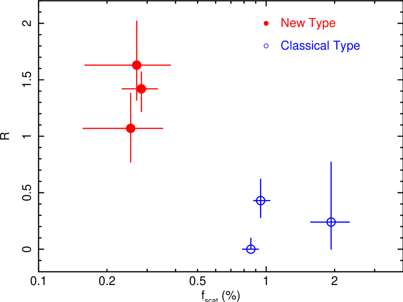
Figure 5.— The correlation between the strength of the Compton reflection component ($R=\Omega/2\pi$) and the fraction of the scattered component ($f_{\rm{scat}}$) for the 6 targets. Filled and open circles represent “new type” ($R\gtrsim 0.8$ and $f_{\rm{scat}}\lesssim 0.5\%$) and “classical type” ($R\lesssim 0.8$ and $f_{\rm{scat}}\gtrsim 0.5\%$), respectively.

We have for the first time obtained broad-band spectra covering the 0.5–50 keV band of the six “new” AGNs detected in the Swift/BAT survey that did not have precise X-ray observations, including the two sources already reported by Ueda et al. (2007). These six targets were essentially selected without biases, and hence can be regarded as a representative sample of new Swift/BAT AGNs. The spectra of all the targets are uniformly described with a spectral model consisting of a heavily absorbed (log $N_{\rm H}>23.5$ cm^-2) transmitted components with a single or multiple absorptions, scattered lights, a Compton reflection component from optically-thick cold matter, and an iron-K emission line at 6.4 keV in the rest-frame, with additional soft X-ray components in two cases. Thanks to its good sensitivity in the 10–50 keV band and simultaneous band coverage with Suzaku, we have accurately derived key spectral parameters including the fraction of the scattered component $f_{\rm scat}$, the strength of the reflection component $R(=\Omega/2\pi)$, and the E.W. of the iron-K emission line.

The first notable result is that our sample show very small values of $f_{\rm{scat}}$, $<3\%$, compared with a typical value of optical selected Seyfert-2 samples of 3–10% (e.g., Turner et al., 1997; Cappi et al., 2006; Guainazzi et al., 2005). Winter et al. (2008b) categorize AGNs with $f_{\rm scat}<3\%$ as “hidden” AGNs, to which all the six sources belong. This is not unexpected, since the “hidden” AGNs constitutes a significant fraction (24%) of the uniform Swift/BAT sample.

Figure 5 shows the correlation between the reflection strength $R$ versus scattering fraction $f_{\rm{scat}}$ for our sample. This plot suggests that there are two groups even within the “hidden” population defined by Winter et al. 2008b, that is,

• $R\gtrsim 0.8$ and $f_{\rm{scat}}\lesssim 0.5\%$

• $R\lesssim 0.8$ and $f_{\rm{scat}}\gtrsim 0.5\%$,

although it is hard to conclude if this distribution is really distinct or continuous, given the small number of the current sample. Following the description by Ueda et al. (2007), we refer to the former group as “new type” and the other “classical type”. The new group includes the two sources of Ueda et al. (2007), Swift J0138.6–4001 and Swift J0601.9–8636, and Swift J0255.2–0011. The extremely small scattering fraction indicates two possibilities (1) the opening angle of the torus is small and/or (2) there is very little gas around the torus to scatter the X-rays. Although it is difficult to firmly exclude the latter possibility, the global presence of a reflection component strongly supports the former, as discussed below.

We can constrain the geometry of the torus and viewing angles from the spectral parameters, the scattering fraction, the E.W. of the iron-K line, and absorption column density, based on a simple torus model. Here we utilize the calculation by Levenson et al. (2002), where three free parameters are introduced for a uniform-density torus whose cross-section has a square shape; the thickness of the torus in terms of the optical depth for Thomson scattering $\tau$, the half-opening angle of torus $\theta$, and the inclination angle $i$. In this geometry, the line-of-sight column density of the torus depends on $i$; when we see the nucleus with face-on view, the absorption becomes much smaller than the case of edge-on view. If the column density of the scatterer is constant, the opening angle can be connected to the scattering fraction as

$$\cos\theta=1-\frac{f_{\rm{scat}}}{f_{\rm{scat,0}}}\left(1-\cos\theta_{0}\right).$$ (2)

where we normalize $f_{\rm{scat}}=f_{\rm{scat},0}$ at $\theta=\theta_{0}$. Assuming $f_{\rm{scat,0}}=3\%$ at $\theta_{0}=45^{\circ}$ as typical parameters , we obtain $\theta\sim 20^{\circ}$ for the new type group. Then, comparing with Figure 2 of Levenson et al. (2002) where $\tau=4$ is assumed, we can constrain $i\sim 40^{\circ}$ for Swift J0601.9–8636, and $i\sim 20^{\circ}$ for Swift J0138.6–4001 and Swift J0255.2–0011, from the observed E.W. of the iron-K line (here we have neglected the contribution of an iron-K line originating from the accretion disk, which is often broader than the “narrow” one considered in the spectral model.). The absorption column densities $N_{\rm{H}}$ $\gtrsim 10^{23.8}\ \rm{cm}^{-2}$ and strong reflection $R\gtrsim 1$ are fully consistent with the geometry considered here. The reflection continuum is attributable to that from the inner wall of the tall torus and that from the accretion disk seen with a small inclination angle.

Thus, it is very likely that we are seeing the new type AGNs in a rather face-on geometry through a geometrically and optically thick torus, as discussed in Ueda et al. (2007). An important consequence of this interpretation is that, if we view the same objects in a more edge-on geometry, then these AGNs look heavily Compton-thick ($N_{\rm H}\sim 10^{25}$ cm^-2) and hence the transmitted components hardly escape toward us even in the hard X-ray $>10$ keV regime due to repeated scattering. Thus, simliar systems to new type AGNs discovered here may still be largely missed even in the on-going Swift/BAT or INTEGRAL surveys, requiring even more sensitive observations in hard X-rays to detect them more completely.

For the classical type of AGNs, we obtain $\theta\gtrsim 30^{\circ}$ from the observed scattered fraction by equation (2). Two sources in this group, Swift J0505.7–2348 and Swift J1628.1–5145, show weak E.W. of the iron-K emission line, $\sim 0.05$ keV. This is hard to explain by a torus with large $\tau$ as assumed in Figure 2 of Levenson et al. (2002), which predicts E.W. $>0.1$ keV if $i>\theta$ (i.e., the transmitted component is absorbed). To consider a torus with different optical depths, we apply a model developed by Ghisellini et al. (1994) (see their Figure 1 for the definition of the geometry). We find that the E.W of the iron-K line and absorption can be consistently explained, within a factor of 2, if the column density of the torus in the equatorial plane is $\sim 10^{23-24}$ cm^-2 and $60^{\circ}\leq i\leq 84^{\circ}$. The absence of strong reflection components is also consistent with the small optical depth of the torus and with the “edge-on” accretion disk.

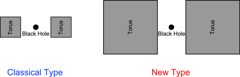
Figure 6.— The schematic illustration of the torus geometry for the classical type AGNs (left panel) and the new type AGNs (right panel).

To summarize, we have discovered from our first Swift-Suzaku AGN sample two different classes of obscured AGN population, called “new type” that have an extremely small scattering fraction ($f_{\rm scat}<0.5\%$) and a strong reflection component ($R\gtrsim 0.8$), and “classical type” with $f_{\rm scat}>0.5\%$ and $R\lesssim 0.8$. Figure 6 shows a schematic illustration of the torus geometry of the two types. It is likely that the new type AGNs are deeply buried in an optically thick torus ($N_{\rm H}\sim 10^{25}$ cm^-2) with a small opening angle $\theta\sim 20^{\circ}$, and are viewed in a face-on geometry. By contrast, the classical type AGNs have an optically thin torus ($N_{\rm H}\sim 10^{23-24}$ cm^-2) with a larger opening angle $\theta\gtrsim 30^{\circ}$ viewed in a more edge-on geometry than the new type. A significant number of new type AGNs with an edge-on view from us may still be missing in the current all-sky hard X-ray surveys. The presence of two classes of obscured AGNs implies that the understanding of AGN is not as simple as assumed in the population synthesis models of the cosmic X-ray background. Given the small number of our sample, however, it is not clear whether there are two “distinct” types of obscured AGNs or the distribution is continuous. More systematic follow-up observations with Suzaku of new Swift/BAT AGNs are important to establish the true properties of local AGNs.

Table 4Best-fit Spectral Parameters

	SWIFT	J0138.6–4001	J0255.2–0011	J0350.1–5019	J0505.7–2348	J0601.9–8636	J1628.1$+$5145
	Best-fit model	B	B + apec	C	C	B	C
(1)	$N_{\rm{H}}^{\rm{Gal}}$ ($10^{22}\ \rm{cm}^{-2}$)	$0.0163$	$0.0581$	$0.0116$	$0.0212$	$0.102$	$0.0183$
(2)	$N_{\rm{H}}$ or $N_{\rm{H}}^{\rm{a}}$ ($10^{22}\ \rm{cm}^{-2}$)	$65.1^{+4.2}_{-4.6}$	$63.1^{+2.1}_{-1.8}$	$85\pm 16$	$29.3\pm 6.2$	$115^{+23}_{-18}$	$58\pm 11$
(3)	$N_{\rm{H}}^{\rm{b}}$ ($10^{22}\ \rm{cm}^{-2}$)	—	—	$8.8^{+3.0}_{-2.1}$	$5.868\pm 0.081$	—	$12.91^{+0.36}_{-0.45}$
(4)	$f_{\rm{c}}$	—	—	$0.877^{+0.033}_{-0.037}$	$0.261^{+0.057}_{-0.023}$	—	$0.380^{+0.036}_{-0.039}$
(5)	$\Gamma$	$1.755^{+0.081}_{-0.048}$	$1.7778\pm 0.022$	$1.900^{+0.064}_{-0.070}$	$1.621^{+0.021}_{-0.032}$	$1.962^{+0.066}_{-0.064}$	$1.799^{+0.030}_{-0.029}$
(6)	$f_{\rm{scat}}$ (%)	$0.276^{+0.070}_{-0.068}$	$0.263\pm 0.046$	$2.03^{+0.38}_{-0.41}$	$0.857^{+0.067}_{-0.070}$	$0.27\pm 0.11$	$0.946^{+0.074}_{-0.078}$
(7)	$E_{\rm{cen}}$ (keV)	$6.375^{+0.026}_{-0.030}$	$6.3911\pm 0.0089$	$6.40^{+0.20}_{-0.04}$	$6.392\pm 0.019$	$6.401^{+0.013}_{-0.012}$	$6.275^{+0.067}_{-0.051}$
(8)	E.W. (keV)	$0.167\pm 0.042$	$0.218\pm 0.020$	$0.28^{+0.13}_{-0.14}$	$0.062^{+0.012}_{-0.011}$	$1.14\pm 0.16$	$0.051\pm 0.021$
(9)	$N_{\rm{H}}^{\rm{refl}}$ ($10^{22}\ \rm{cm}^{-2}$)	$8.5^{+2.8}_{-2.7}$	$12.4^{+1.9}_{-1.2}$	$7.3$ ($>0$)	($=N_{\rm{H}}^{\rm{b}}$)	$3.7^{+3.1}_{-1.4}$	($=N_{\rm{H}}^{\rm{b}}$)
(10)	$R$	$1.00^{+0.36}_{-0.26}$	$1.49^{+0.15}_{-0.23}$	$0.28$ ($<0.92$)	$1.4\times 10^{-7}$ ($<9.8\times 10^{-2}$)	$1.63^{+0.39}_{-0.32}$	$0.43^{+0.22}_{-0.16}$
(11)	$F_{\rm{2-10}}$ ($\rm{ergs}\,\rm{cm}^{-2}\,\rm{s}^{-1}$)	$3.4\times 10^{-12}$	$4.2\times 10^{-12}$	$9.2\times 10^{-13}$	$1.1\times 10^{-11}$	$1.0\times 10^{-12}$	$9.0\times 10^{-12}$
(12)	$F_{\rm{10-50}}$ ($\rm{ergs}\,\rm{cm}^{-2}\,\rm{s}^{-1}$)	$3.4\times 10^{-11}$	$4.3\times 10^{-11}$	$5.5\times 10^{-12}$	$2.9\times 10^{-11}$	$1.1\times 10^{-11}$	$3.6\times 10^{-11}$
(13)	$L_{\rm{2-10}}$ ($\rm{ergs}\,\rm{s}^{-1}$)	$2.4\times 10^{43}$	$5.1\times 10^{43}$	$1.4\times 10^{43}$	$1.5\times 10^{44}$	$8.9\times 10^{41}$	$1.5\times 10^{44}$
	$\chi^{2}/\rm{d.o.f.}$	$94.42/97$	$335.97/307$	$27.28/39$	$622.38/604$	$35.48/38$	$558.76/550$

Note. — (1) The hydrogen column density of Galactic absorption by Kalberla et al. (2005). (2) The line-of-sight hydrogen column density for the transmitted component. For the double covering model (Model C), that for more heavily absorbed component is given. (3) The smaller line-of-sight hydrogen column density for the transmitted component in Model C. (4) The normalization fraction of the more absorbed component to the total transmitted one in Model C. (5) The power-law photon index. (6) The fraction of the scattered component relative to the intrinsic power law,corrected for the transmission efficiency of $1/R$ if $R>1$ (see text). (7) The center energy of the iron-K emission line at the rest frame of the source redshift. (8) The observed equivalent width of the iron-K line with respect to the whole continuum. (9) The line-of-sight hydrogen column density for the reflection component. (10) The relative strength of the reflection component to the transmitted one, defined as $R\equiv\Omega/2\pi$, where $\Omega$ is the solid angle of the reflector viewed from the nucleus. (11) The observed flux in the 2–10 keV band. (12) The observed flux in the 10–50 keV band. (13) The 2–10 keV intrinsic luminosity corrected for the absorption and the transmission efficiency of $1/R$ if $R>1$. The errors are 90% confidence limits for a single parameter.

References

- Anders & Grevesse (1989) Anders, E., & Grevesse, N. 1989, Geochim. Cosmochim. Acta, 53, 197
- Balucinska-Church & McCammon (1992) Balucinska-Church, M. & McCammon, D. 1992, ApJ, 400, 699
- Bassani et al. (2006) Bassani, L., et al. 2006, ApJ, 636, L65
- Cappi et al. (2006) Cappi, M., et al. 2006, A&A, 446, 459
- Comastri et al. (1998) Comastri, A., Vignali, C., Cappi, M., Matt, G., Audano, R., Awaki, H., & Ueno, S. 1998, MNRAS, 295, 443
- Dotani et al. (2007) Dotani, T. & the XIS team 2007, JX-ISAS-SUZAKU-MEMO-2007-08
- Ghisellini et al. (1994) Ghisellini, G., Haardt, F., & Matt, G. 1994, MNRAS, 267, 743
- Gilli et al. (2007) Gilli, R., Comastri, A., & Hasinger, G. 2007, A&A, 463, 79
- Guainazzi et al. (2005) Guainazzi, M., Matt, G., & Perola, G. C. 2005, A&A, 444, 119
- Hasinger (2008) Hasinger, G. 2008, A&A, 490, 905
- Hopkins et al. (2006) Hopkins, P. F., Hernquist, L., Cox, T. J., Di Matteo, T., Robertson, B., & Springel, V. 2006, ApJS, 163, 1
- Ishida et al. (2007) Ishida, M., Suzuki, K., & Someya, K., 2007, JX-ISAS-SUZAKU-MEMO-2007-11
- Kalberla et al. (2005) Kalberla, P. M. W., Burton, W. B., Hartmann, D., Arnal, E. M., Bajaja, E., Morras, R., Pöppel, W. G. L. 2005, A&A, 440, 775
- Koyama et al. (2007) Koyama, K., et al. 2007, PASJ, 59, 23
- Krivonos et al. (2007) Krivonos, R., Revnivtsev, M., Lutovinov, A., Sazonov, S., Churazov, E., & Sunyaev, R. 2007, A&A, 475, 775
- Levenson et al. (2002) Levenson, N. A., Krolik, J. H., Życki, P. T., Heckman, T. M., Weaver, K. A., Awaki, H., & Terashima, Y. 2002, ApJ, 573, L81
- Magdziarz & Zdziarski (1995) Magdziarz, P., & Zdziarski, A. A. 1995, MNRAS, 273, 837
- Maiolino et al. (2003) Maiolino, R., et al. 2003, MNRAS, 344, L59
- Matsumoto (2007) Matsumoto, H. & the XIS team, 2007, JX-ISAS-SUZAKU-MEMO-2007-06
- Matt et al. (1991) Matt, G., Perola, G. C., & Piro, L. 1991, A&A, 247, 25
- Matt et al. (2004) Matt, G., Bianchi, S., D’Ammando, F., & Martocchia, A. 2004, A&A, 421, 473
- Mitsuda et al. (2007) Mitsuda, K., et al. 2007, PASJ, 59, 1
- Mizuno et al. (2008) Mizuno, T., et al. 2008, JX-ISAS-SUZAKU-MEMO-2008-03
- Nakajima et al. (2008) Nakajima, H., et al. 2008, PASJ, 60, 1
- Ogle et al. (2000) Ogle, P. M., Marshall, H. L., Lee, J. C., & Canizares, C. R. 2000, ApJ, 545, L81
- Sako et al. (2000) Sako, M., Kahn, S. M., Paerels, F., & Liedahl, D. A. 2000, ApJ, 543, L115
- Takahashi et al. (2007) Takahashi, T., et al. 2007, PASJ, 59, 35
- Tueller et al. (2008) Tueller, J., Mushotzky, R. F., Barthelmy, S., Cannizzo, J. K., Gehrels, N., Markwardt, C. B., Skinner, G. K., & Winter, L. M. 2008, ApJ, 681, 113
- Turner et al. (1997) Turner, T. J., George, I. M., Nandra, K., & Mushotzky, R. F. 1997, ApJS, 113, 23
- Ueda et al. (2003) Ueda, Y., Akiyama, M., Ohta, K., & Miyaji, T. 2003, ApJ, 598, 886
- Ueda et al. (2007) Ueda, Y., et al. 2007, ApJ, 664, L79
- Wada & Norman (2002) Wada, K., & Norman, C. A. 2002, ApJ, 566, L21
- Winter et al. (2008a) Winter, L. M., Mushotzky, R. F., Tueller, J., & Markwardt, C. 2008a, ApJ, 674, 686
- Winter et al. (2008b) Winter, L. M., Mushotzky, R., Reynolds, C. S., & Tueller, J. 2008b, arXiv:0808.0461