Serre Relation and Higher Grade Generators
of the AdS/CFT Yangian Symmetry

It was shown that the spin chain model coming from AdS/CFT correspondence satisfies the Yangian symmetry if we assume evaluation representation, though so far there is no explicit proof that the evaluation representation satisfies the Serre relation, which is one of the defining equations of the Yangian algebra imposing constraints on the whole algebraic structure. We prove completely that the evaluation representation adopted in the model satisfies the Serre relation by introducing a three-dimensional gamma matrix. After studying the Serre relation, we proceed to the whole Yangian algebraic structure, where we find that the conventional construction of higher grade generators is singular and we propose an alternative construction. In the discussion of the higher grade generators, a great simplification for the proof of the Serre relation is found. Using this expression, we further show that the proof is lifted to the exceptional superalgebra, which is a non-degenerate deformation of the original superalgebra.

1 Introduction

It is no doubt that Yang-Mills theory plays important roles in understanding the modern particle physics. Especially, the maximally super Yang-Mills theory enjoys an interesting theoretical property. Since the maximally super Yang-Mills theory is conjectured to be dual to string theory on $AdS_{5}\times S^{5}$ with RR flux background [1], it is expected that the super Yang-Mills theory can be used to describe string theory as various matrix models describe various string theories.

In this context, it is exciting to find [2] that the one-loop anomalous dimension of Yang-Mills theory is mapped explicitly to the Hamiltonian of an integrable spin chain model, because infinite generators of the integrable model may play a central role in studying string theory on the curved spacetime, as the Virasoro generators play on the flat spacetime. Therefore, it is aspiring to understand the whole integrable algebraic structure with infinite generators completely.

The analysis is pushed further to the all-loop level. Fixing one direction as the vacuum, the original dynamic spin chain of the superconformal symmetry $\mathfrak{psu}(2,2|4)$ is broken down to two copies of undynamic ones of $\mathfrak{psu}(2|2)$ with some common central charges [6, 7]. Especially, an off-shell formalism with the centrally extended superalgebra $\mathfrak{psu}(2|2)\ltimes{\mathbb{R}}^{3}$ was proposed in [8]. Then, it is surprising to find that the R-matrix, which is determined uniquely (up to an overall factor) by requiring this Lie algebraic symmetry $\mathfrak{psu}(2|2)\ltimes{\mathbb{R}}^{3}$, enjoys the Yang-Baxter equation, which implies the integrability. Besides, it was also shown [9] that the R-matrix has the grade-1 Yangian symmetry if we assume the evaluation representation for the Yangian algebra. Later, the Yangian algebra with the evaluation representation also turns out to be crucial in determining the R-matrix of bound states [10].

The Yangian algebra consists of infinitely graded generators ${\mathfrak{J}}^{A}_{n}$. (See [11] for the original work and [12] for a review.) The grade-0 generator ${\mathfrak{J}}^{A}_{0}={\mathfrak{J}}^{A}$ is that of the standard Lie algebra $[{\mathfrak{J}}^{A},{\mathfrak{J}}^{B}]={\mathfrak{J}}^{C}f_{C}{}^{AB}$ (with the superscript on the left and the subscript on the right, as the canonical position of the spinor indices), satisfying the Jacobi identity,

$$[{\mathfrak{J}}^{A},[{\mathfrak{J}}^{B},{\mathfrak{J}}^{C}]]+(-)^{|A|(|B|+|C|)}[{\mathfrak{J}}^{B},[{\mathfrak{J}}^{C},{\mathfrak{J}}^{A}]]+(-)^{|C|(|A|+|B|)}[{\mathfrak{J}}^{C},[{\mathfrak{J}}^{A},{\mathfrak{J}}^{B}]]=0.$$ (1.1)

Note that we consider the superalgebra, where the commutator and the anticommutator (which will appear later) denote the generalized ones $[{\mathfrak{J}}^{A},{\mathfrak{J}}^{B}]={\mathfrak{J}}^{A}{\mathfrak{J}}^{B}-(-)^{|A||B|}{\mathfrak{J}}^{B}{\mathfrak{J}}^{A}$, $\{{\mathfrak{J}}^{A},{\mathfrak{J}}^{B}\}={\mathfrak{J}}^{A}{\mathfrak{J}}^{B}+(-)^{|A||B|}{\mathfrak{J}}^{B}{\mathfrak{J}}^{A}$, with $|A|=0$ $(|A|=1)$ for the bosonic (fermionic) generator ${\mathfrak{J}}^{A}$.

The grade-1 generator ${\mathfrak{J}}^{A}_{1}=\widehat{\mathfrak{J}}^{A}$, with the commutation relations with the Lie algebra generator $[\widehat{\mathfrak{J}}^{A},{\mathfrak{J}}^{B}]=[{\mathfrak{J}}^{A},\widehat{\mathfrak{J}}^{B}]=\widehat{\mathfrak{J}}^{C}f_{C}{}^{AB}$, satisfies further the Serre relation,

$$[\widehat{\mathfrak{J}}^{A},[\widehat{\mathfrak{J}}^{B},{\mathfrak{J}}^{C}]]+(-)^{|A|(|B|+|C|)}[\widehat{\mathfrak{J}}^{B},[\widehat{\mathfrak{J}}^{C},{\mathfrak{J}}^{A}]]+(-)^{|C|(|A|+|B|)}[\widehat{\mathfrak{J}}^{C},[\widehat{\mathfrak{J}}^{A},{\mathfrak{J}}^{B}]]$$

$$\quad=-\frac{\hbar^{2}}{24}(-)^{|I|(|B|+|J|+|C|+|K|)+|J|(|C|+|K|)}\{{\mathfrak{J}}^{L},{\mathfrak{J}}^{M},{\mathfrak{J}}^{N}\}f_{L}{}^{AI}f_{M}{}^{BJ}f_{N}{}^{CK}f_{IJK},$$ (1.2)

where the generalized totally symmetrized product is

$$\{{\mathfrak{J}}^{L},{\mathfrak{J}}^{M},{\mathfrak{J}}^{N}\}=\{{\mathfrak{J}}^{L},{\mathfrak{J}}^{M}\}{\mathfrak{J}}^{N}+(-)^{|L|(|M|+|N|)}\{{\mathfrak{J}}^{M},{\mathfrak{J}}^{N}\}{\mathfrak{J}}^{L}+(-)^{|N|(|L|+|M|)}\{{\mathfrak{J}}^{N},{\mathfrak{J}}^{L}\}{\mathfrak{J}}^{M}.$$ (1.3)

Here the complicated-looking sign $(-)^{|I|(|B|+|J|+|C|+|K|)+|J|(|C|+|K|)}$ in (1.2) can be simply interpreted as the Grassmannian charge which appears if we exchange the order of the indices to contract the subscripts $I,J,K$ in $f_{IJK}$ with the same superscripts in ${\mathfrak{J}}^{L}f_{L}{}^{AI}{\mathfrak{J}}^{M}f_{M}{}^{BJ}{\mathfrak{J}}^{N}f_{N}{}^{CK}$ in the canonical position. Serre relation in the simple Lie algebra imposes constraints on the construction of full root system from the simple roots. Here in the Yangian algebra, the Serre relation (1.2) puts constraints on the construction of higher grade generators. Therefore, it is obvious that the Serre relation is important in studying the whole integrable algebraic structure with the higher grade generators.

Some representations of the Lie algebra $\mathfrak{g}$ admit the evaluation representations for the corresponding Yangian algebra $Y(\mathfrak{g})$, which require the representation of the higher grade generators to relate to that of the Lie algebra by ${\mathfrak{J}}^{A}_{n}\simeq(iu)^{n}{\mathfrak{J}}^{A}$ with the spectral parameter $u$. The physical meaning of the evaluation representation is not very clear, but since the evaluation representation takes a similar appearance as the affine Lie algebra of conformal field theory and since the classical limit of the R-matrix with the Yangian symmetry takes the canonical form

$$r_{12}=\frac{{\mathcal{T}}^{\mathfrak{g}}_{12}}{i(u_{1}-u_{2})}=\sum_{n=0}^{\infty}{\mathfrak{J}}^{A}_{-n-1}\otimes{\mathfrak{J}}_{An},$$ (1.4)

with the two-site Casimir operator ${\mathcal{T}}^{\mathfrak{g}}_{12}={\mathfrak{J}}^{A}\otimes{\mathfrak{J}}_{A}={\mathfrak{J}}^{A}\otimes{\mathfrak{J}}^{B}g_{BA}$, which is reminiscent of the KZ equation of the WZW model, it is natural to expect that the evaluation representation has a close relation with the classical limit of the string worldsheet theory. The classical limit of the $\mathfrak{psu}(2|2)\ltimes{\mathbb{R}}^{3}$ spin chain model was investigated in [13, 14, 15, 16].

Although it was found that the R-matrix has the grade-1 Yangian coproduct symmetry if we adopt the evaluation representation, it has not been shown explicitly so far that the evaluation representation is compatible with the Serre relation. One of the main subjects in this paper is to study the compatibility. Namely, since, in the evaluation representation $\widehat{{\mathfrak{J}}}^{A}\simeq iu{\mathfrak{J}}^{A}$, the left-hand-side of the Serre relation (1.2) reduces to that of the Jacobi identity (1.1), the right-hand-side of the Serre relation (1.2) has to vanish when acting on any states. We will prove it extensively in the following sections.

One reason that this computation has not been done before is because of the degeneracy of the Killing form of the superalgebra $\mathfrak{psu}(2|2)\ltimes{\mathbb{R}}^{3}$. In studying the Serre relation, we have to raise and lower the indices frequently and it is impossible to proceed if the Killing form is degenerate. In [8, 16], it was shown that the algebra is a special limit ($\varepsilon\to 0$) of the exceptional superalgebra $\mathfrak{d}(2,1;\varepsilon)$ with a parameter $\varepsilon$, whose Killing form is non-degenerate and, therefore, many algebraic properties can be studied in this $\varepsilon$-deformation. Motivated by its non-degeneracy, we also constructed an infinite-dimensional representation of the exceptional superalgebra $\mathfrak{d}(2,1;\varepsilon)$ in [16], which is a natural lift of the fundamental representation of the superalgebra $\mathfrak{psu}(2|2)\ltimes{\mathbb{R}}^{3}$.

Another difficulty is due to the complexity of the structure constants. In order to study the Serre relation, let us read off the Killing form $g_{AB}$ from the two-site Casimir operator,

$${\mathcal{T}}^{\mathfrak{d}}_{12}=-\alpha{\mathfrak{R}}^{a}{}_{b}\otimes{\mathfrak{R}}^{b}{}_{a}-\beta{\mathfrak{L}}^{\alpha}{}_{\beta}\otimes{\mathfrak{L}}^{\beta}{}_{\alpha}-\gamma{\mathfrak{C}}^{\mathfrak{a}}{}_{\mathfrak{b}}\otimes{\mathfrak{C}}^{\mathfrak{b}}{}_{\mathfrak{a}}-\epsilon_{ab}\epsilon_{\alpha\beta}\epsilon_{\mathfrak{a}\mathfrak{b}}{\mathfrak{F}}^{a\alpha\mathfrak{a}}\otimes{\mathfrak{F}}^{b\beta\mathfrak{b}},$$ (1.5)

and spell out the non-zero structure constant from the commutation relations

$$f_{{\mathfrak{R}}^{a}{}_{a^{\prime}}{\mathfrak{R}}^{b}{}_{b^{\prime}}{\mathfrak{R}}^{c}{}_{c^{\prime}}} =\alpha^{2}(\delta_{a}^{b^{\prime}}\delta_{b}^{c^{\prime}}\delta_{c}^{a^{\prime}}-\delta_{a}^{c^{\prime}}\delta_{b}^{a^{\prime}}\delta_{c}^{b^{\prime}}), f_{{\mathfrak{F}}^{a\alpha\mathfrak{a}}{\mathfrak{F}}^{b\beta\mathfrak{b}}{\mathfrak{R}}^{c}{}_{c^{\prime}}} =\frac{\alpha}{2}(\epsilon_{ac}\delta^{c^{\prime}}_{b}+\epsilon_{bc}\delta^{c^{\prime}}_{a})\epsilon_{\alpha\beta}\epsilon_{\mathfrak{a}\mathfrak{b}},$$

$$f_{{\mathfrak{L}}^{\alpha}{}_{\alpha^{\prime}}{\mathfrak{L}}^{\beta}{}_{\beta^{\prime}}{\mathfrak{L}}^{\gamma}{}_{\gamma^{\prime}}} =\beta^{2}(\delta_{\alpha}^{\beta^{\prime}}\delta_{\beta}^{\gamma^{\prime}}\delta_{\gamma}^{\alpha^{\prime}}-\delta_{\alpha}^{\gamma^{\prime}}\delta_{\beta}^{\alpha^{\prime}}\delta_{\gamma}^{\beta^{\prime}}), f_{{\mathfrak{F}}^{a\alpha\mathfrak{a}}{\mathfrak{F}}^{b\beta\mathfrak{b}}{\mathfrak{L}}^{\gamma}{}_{\gamma^{\prime}}} =\frac{\beta}{2}\epsilon_{ab}(\epsilon_{\alpha\gamma}\delta^{\gamma^{\prime}}_{\beta}+\epsilon_{\beta\gamma}\delta^{\gamma^{\prime}}_{\alpha})\epsilon_{\mathfrak{a}\mathfrak{b}},$$

$$f_{{\mathfrak{C}}^{\mathfrak{a}}{}_{\mathfrak{a}^{\prime}}{\mathfrak{C}}^{\mathfrak{b}}{}_{\mathfrak{b}^{\prime}}{\mathfrak{C}}^{\mathfrak{c}}{}_{\mathfrak{c}^{\prime}}} =\gamma^{2}(\delta_{\mathfrak{a}}^{\mathfrak{b}^{\prime}}\delta_{\mathfrak{b}}^{\mathfrak{c}^{\prime}}\delta_{\mathfrak{c}}^{\mathfrak{a}^{\prime}}-\delta_{\mathfrak{a}}^{\mathfrak{c}^{\prime}}\delta_{\mathfrak{b}}^{\mathfrak{a}^{\prime}}\delta_{\mathfrak{c}}^{\mathfrak{b}^{\prime}}), f_{{\mathfrak{F}}^{a\alpha\mathfrak{a}}{\mathfrak{F}}^{b\beta\mathfrak{b}}{\mathfrak{C}}^{\mathfrak{c}}{}_{\mathfrak{c}^{\prime}}} =\frac{\gamma}{2}\epsilon_{ab}\epsilon_{\alpha\beta}(\epsilon_{\mathfrak{a}\mathfrak{c}}\delta^{\mathfrak{c}^{\prime}}_{\mathfrak{b}}+\epsilon_{\mathfrak{b}\mathfrak{c}}\delta^{\mathfrak{c}^{\prime}}_{\mathfrak{a}}).$$ (1.6)

If we plug these structure constants into the Serre relation, we can easily get stranded because of the complexity of $2^{4}=16$ terms, which comes from four structure constants with each consisting of two terms.

In this paper, we shall regard $\mathfrak{su}(2)$ as $\mathfrak{so}(3)$ and define a three-dimensional gamma matrix. Then, all of the structure constants (1.6) can be rewritten in a simple form in terms of the gamma matrix. With lots of formulas of the gamma matrix, the computation can be done without difficulty as that of scattering amplitudes of fermions.

After proving that the evaluation representation is compatible with the Serre relation, we proceed to construct higher grade generators. We find a novel subtle structure, suggesting that the canonical expression of the higher grade generators has to be improved. We propose a resolution to this subtlety. Our resolution further implies a great simplification for the proof of the compatibility. Hence, subsequently, we come back to the non-degenerate deformation of the exceptional superalgebra $\mathfrak{d}(2,1;\varepsilon)$ and prove that the compatibility of the evaluation representation is also lifted the exceptional superalgebra $\mathfrak{d}(2,1;\varepsilon)$.

In the next section, after recapitulating the algebra shortly, we reformulate the algebra and the representation by introducing a three-dimensional gamma matrix. Then, in section 3, we prove that the evaluation representation is compatible with the Serre relation. After the proof, we proceed to the higher grade generators in section 4. And in section 5 we present a proof of the compatibility for the case of the exceptional superalgebra. Finally, we conclude in section 6. In appendix A, we show how the Serre relation relates to the homomorphism of the coproduct. The subsequent three appendices are devoted to various useful formulas in computation.

2 Gamma matrix formalism

We shall introduce a three-dimensional gamma matrix and reformulate the exceptional Lie superalgebra $\mathfrak{d}(2,1;\varepsilon)$, its $\varepsilon\to 0$ limit $\mathfrak{psu}(2|2)\ltimes{\mathbb{R}}^{3}$ and their representations [8, 16] in terms of the gamma matrix.

2.1 Algebra

The generators of the exceptional Lie superalgebra $\mathfrak{d}(2,1;\varepsilon)$ consist of three orthogonal sets of $\mathfrak{su}(2)$ triplet bosonic generators ${\mathfrak{R}}^{a}{}_{b}$, ${\mathfrak{L}}^{\alpha}{}_{\beta}$, ${\mathfrak{C}}^{\mathfrak{a}}{}_{\mathfrak{b}}$ (subject to the traceless condition ${\mathfrak{R}}^{a}{}_{a}={\mathfrak{L}}^{\alpha}{}_{\alpha}={\mathfrak{C}}^{\mathfrak{a}}{}_{\mathfrak{a}}=0$) and an octet of fermionic generators ${\mathfrak{F}}^{a\alpha\mathfrak{a}}$ where all indices $a,\alpha,\mathfrak{a}$ run over $1$ and $2$. The non-trivial commutation relations are given as

$$[{\mathfrak{R}}^{a}{}_{b},{\mathfrak{R}}^{c}{}_{d}]=\delta^{c}_{b}{\mathfrak{R}}^{a}{}_{d}-\delta^{a}_{d}{\mathfrak{R}}^{c}{}_{b},\;[{\mathfrak{L}}^{\alpha}{}_{\beta},{\mathfrak{L}}^{\gamma}{}_{\delta}]=\delta^{\gamma}_{\beta}{\mathfrak{L}}^{\alpha}{}_{\delta}-\delta^{\alpha}_{\delta}{\mathfrak{L}}^{\gamma}{}_{\beta},\;[{\mathfrak{C}}^{\mathfrak{a}}{}_{\mathfrak{b}},{\mathfrak{C}}^{\mathfrak{c}}{}_{\mathfrak{d}}]=\delta^{\mathfrak{c}}_{\mathfrak{b}}{\mathfrak{C}}^{\mathfrak{a}}{}_{\mathfrak{d}}-\delta^{\mathfrak{a}}_{\mathfrak{d}}{\mathfrak{C}}^{\mathfrak{c}}{}_{\mathfrak{b}},$$

$$[{\mathfrak{R}}^{a}{}_{b},{\mathfrak{F}}^{c\gamma\mathfrak{c}}]=\delta^{c}_{b}{\mathfrak{F}}^{a\gamma\mathfrak{c}}-\frac{1}{2}\delta^{a}_{b}{\mathfrak{F}}^{c\gamma\mathfrak{c}},\;[{\mathfrak{L}}^{\alpha}{}_{\beta},{\mathfrak{F}}^{c\gamma\mathfrak{c}}]=\delta^{\gamma}_{\beta}{\mathfrak{F}}^{c\alpha\mathfrak{c}}-\frac{1}{2}\delta^{\alpha}_{\beta}{\mathfrak{F}}^{c\gamma\mathfrak{c}},\;[{\mathfrak{C}}^{\mathfrak{a}}{}_{\mathfrak{b}},{\mathfrak{F}}^{c\gamma\mathfrak{c}}]=\delta^{\mathfrak{c}}_{\mathfrak{b}}{\mathfrak{F}}^{c\gamma\mathfrak{a}}-\frac{1}{2}\delta^{\mathfrak{a}}_{\mathfrak{b}}{\mathfrak{F}}^{c\gamma\mathfrak{c}},$$

$$[{\mathfrak{F}}^{a\alpha\mathfrak{a}},{\mathfrak{F}}^{b\beta\mathfrak{b}}]=\alpha\epsilon^{ak}\epsilon^{\alpha\beta}\epsilon^{\mathfrak{a}\mathfrak{b}}{\mathfrak{R}}^{b}{}_{k}+\beta\epsilon^{ab}\epsilon^{\alpha\kappa}\epsilon^{\mathfrak{a}\mathfrak{b}}{\mathfrak{L}}^{\beta}{}_{\kappa}+\gamma\epsilon^{ab}\epsilon^{\alpha\beta}\epsilon^{\mathfrak{a}\mathfrak{k}}{\mathfrak{C}}^{\mathfrak{b}}{}_{\mathfrak{k}}.$$ (2.1)

where the constants $\alpha$, $\beta$, $\gamma$ have to satisfy $\alpha+\beta+\gamma=0$ due to the Jacobi identity. Since the overall rescaling does not change the algebraic structure, the only one relevant parameter which characterizes $\mathfrak{d}(2,1;\varepsilon)$ is $\varepsilon=-\gamma/\alpha$. This exceptional algebra has a well-defined two-site quadratic Casimir operator (1.5), which enables many studies of the algebraic properties [16]. To reproduce the centrally extended superalgebra $\mathfrak{psu}(2|2)\ltimes{\mathbb{R}}^{3}$ without encountering the singular behavior, we shall rewrite

$$\alpha=-1,\quad\beta=1-\varepsilon,\quad\gamma=\varepsilon,\quad{\mathfrak{C}}^{\mathfrak{a}}{}_{\mathfrak{b}}=\overline{{\mathfrak{C}}}{}^{\mathfrak{a}}{}_{\mathfrak{b}}/\varepsilon.$$ (2.2)

for the parameters $\alpha$, $\beta$, $\gamma$ and the last bosonic $\mathfrak{su}(2)$ generator ${\mathfrak{C}}^{\mathfrak{a}}{}_{\mathfrak{b}}$ (which becomes the centers of $\mathfrak{psu}(2|2)\ltimes{\mathbb{R}}^{3}$) and take the limit $\varepsilon\to 0$.

Now let us regard each of three orthogonal sets of $\mathfrak{su}(2)$ as $\mathfrak{so}(3)$ and define three kinds of three-dimensional gamma matrices $(\gamma^{\boldsymbol{A}})^{K}{}_{L}=(\gamma^{A}_{A^{\prime}})^{K}{}_{L}$ (where the uppercase latin character $\boldsymbol{A}=(A,A^{\prime})$ denotes either of the lowercase latin character $\boldsymbol{a}=(a,a^{\prime})$, the greek character $\boldsymbol{\alpha}=(\alpha,\alpha^{\prime})$ or the german character $\boldsymbol{\mathfrak{a}}=(\mathfrak{a},\mathfrak{a}^{\prime})$) as

$$(\gamma^{\boldsymbol{A}})^{K}{}_{L}=(\gamma^{A}_{A^{\prime}})^{K}{}_{L}=\frac{1}{\sqrt{2}}\epsilon^{KM}(\epsilon_{MA^{\prime}}\delta^{A}_{L}+\epsilon_{LA^{\prime}}\delta^{A}_{M})=-\sqrt{2}\Bigl{(}\delta^{K}_{A^{\prime}}\delta^{A}_{L}-\frac{1}{2}\delta^{K}_{L}\delta^{A}_{A^{\prime}}\Bigr{)}.$$ (2.3)

Then, the gamma matrix satisfies the canonical Clifford algebra,

$$(\gamma^{\boldsymbol{A}})^{K}{}_{L}(\gamma^{\boldsymbol{B}})^{L}{}_{M}+(\gamma^{\boldsymbol{B}})^{K}{}_{L}(\gamma^{\boldsymbol{A}})^{L}{}_{M}=2\delta^{K}_{M}g^{\boldsymbol{A}\boldsymbol{B}},$$ (2.4)

with the metric defined as

$$g^{\boldsymbol{A}\boldsymbol{B}}=\delta^{B}_{A^{\prime}}\delta^{A}_{B^{\prime}}-\frac{1}{2}\delta^{A}_{A^{\prime}}\delta^{B}_{B^{\prime}},\quad g_{\boldsymbol{A}\boldsymbol{B}}=\delta^{B^{\prime}}_{A}\delta^{A^{\prime}}_{B}-\frac{1}{2}\delta^{A^{\prime}}_{A}\delta^{B^{\prime}}_{B},\quad\delta^{\boldsymbol{A}}_{\boldsymbol{B}}=\delta^{B^{\prime}}_{A^{\prime}}\delta^{A}_{B}-\frac{1}{2}\delta^{A}_{A^{\prime}}\delta^{B^{\prime}}_{B}.$$ (2.5)

Note that in the metric we subtract the trace part, so that the degree of freedom is $\delta^{\boldsymbol{A}}_{\boldsymbol{A}}=3$, which matches the dimension of the adjoint representation of $\mathfrak{su}(2)$. Note also that $(\gamma^{\boldsymbol{A}}\epsilon)^{KL}=(\gamma^{\boldsymbol{A}})^{K}{}_{M}\epsilon^{ML}$ and $(\epsilon\gamma^{\boldsymbol{A}})_{KL}=\epsilon_{KM}(\gamma^{\boldsymbol{A}})^{M}{}_{L}$ are symmetric under the exchange of $K$ and $L$, while the symmetry of the product of two gamma matrices reads $(\gamma^{\boldsymbol{A}}\gamma^{\boldsymbol{B}}\epsilon)^{KL}=-(\gamma^{\boldsymbol{B}}\gamma^{\boldsymbol{A}}\epsilon)^{LK}$.

Using these gamma matrices, the structure constants now take a simple form

$$f_{{\mathfrak{R}}^{\boldsymbol{c}}}{}^{{\mathfrak{R}}^{\boldsymbol{a}}{\mathfrak{R}}^{\boldsymbol{b}}} =\frac{1}{\sqrt{2}}{\rm Tr}(\gamma_{\boldsymbol{c}}\gamma^{\boldsymbol{a}}\gamma^{\boldsymbol{b}}), f_{{\mathfrak{F}}^{c\gamma\mathfrak{c}}}{}^{{\mathfrak{R}}^{\boldsymbol{a}}{\mathfrak{F}}^{b\beta\mathfrak{b}}} =\frac{-1}{\sqrt{2}}(\gamma^{\boldsymbol{a}})^{b}{}_{c}\delta^{\beta}_{\gamma}\delta^{\mathfrak{b}}_{\mathfrak{c}}, f_{{\mathfrak{R}}^{\boldsymbol{c}}}{}^{{\mathfrak{F}}^{a\alpha\mathfrak{a}}{\mathfrak{F}}^{b\beta\mathfrak{b}}} =\frac{\alpha}{\sqrt{2}}(\gamma_{\boldsymbol{c}}\epsilon)^{ab}\epsilon^{\alpha\beta}\epsilon^{\mathfrak{a}\mathfrak{b}},$$

$$f_{{\mathfrak{L}}^{\boldsymbol{\gamma}}}{}^{{\mathfrak{L}}^{\boldsymbol{\alpha}}{\mathfrak{L}}^{\boldsymbol{\beta}}} =\frac{1}{\sqrt{2}}{\rm Tr}(\gamma_{\boldsymbol{\gamma}}\gamma^{\boldsymbol{\alpha}}\gamma^{\boldsymbol{\beta}}), f_{{\mathfrak{F}}^{c\gamma\mathfrak{c}}}{}^{{\mathfrak{L}}^{\boldsymbol{\alpha}}{\mathfrak{F}}^{b\beta\mathfrak{b}}} =\frac{-1}{\sqrt{2}}(\gamma^{\boldsymbol{\alpha}})^{\beta}{}_{\gamma}\delta^{b}_{c}\delta^{\mathfrak{b}}_{\mathfrak{c}}, f_{{\mathfrak{L}}^{\boldsymbol{\gamma}}}{}^{{\mathfrak{F}}^{a\alpha\mathfrak{a}}{\mathfrak{F}}^{b\beta\mathfrak{b}}} =\frac{\beta}{\sqrt{2}}(\gamma_{\boldsymbol{\gamma}}\epsilon)^{\alpha\beta}\epsilon^{ab}\epsilon^{\mathfrak{a}\mathfrak{b}},$$

$$f_{{\mathfrak{C}}^{\boldsymbol{\mathfrak{c}}}}{}^{{\mathfrak{C}}^{\boldsymbol{\mathfrak{a}}}{\mathfrak{C}}^{\boldsymbol{\mathfrak{b}}}} =\frac{1}{\sqrt{2}}{\rm Tr}(\gamma_{\boldsymbol{\mathfrak{c}}}\gamma^{\boldsymbol{\mathfrak{a}}}\gamma^{\boldsymbol{\mathfrak{b}}}), f_{{\mathfrak{F}}^{c\gamma\mathfrak{c}}}{}^{{\mathfrak{C}}^{\boldsymbol{\mathfrak{a}}}{\mathfrak{F}}^{b\beta\mathfrak{b}}} =\frac{-1}{\sqrt{2}}(\gamma^{\boldsymbol{\mathfrak{a}}})^{\mathfrak{b}}{}_{\mathfrak{c}}\delta^{b}_{c}\delta^{\beta}_{\gamma}, f_{{\mathfrak{C}}^{\boldsymbol{\mathfrak{c}}}}{}^{{\mathfrak{F}}^{a\alpha\mathfrak{a}}{\mathfrak{F}}^{b\beta\mathfrak{b}}} =\frac{\gamma}{\sqrt{2}}(\gamma_{\boldsymbol{\mathfrak{c}}}\epsilon)^{\mathfrak{a}\mathfrak{b}}\epsilon^{ab}\epsilon^{\alpha\beta},$$ (2.6)

with those whose indices are lowered being

$$f_{{\mathfrak{R}}^{\boldsymbol{a}}{\mathfrak{R}}^{\boldsymbol{b}}{\mathfrak{R}}^{\boldsymbol{c}}} =\frac{\alpha^{2}}{\sqrt{2}}{\rm Tr}(\gamma_{\boldsymbol{a}}\gamma_{\boldsymbol{b}}\gamma_{\boldsymbol{c}}), f_{{\mathfrak{F}}^{a\alpha\mathfrak{a}}{\mathfrak{F}}^{b\beta\mathfrak{b}}{\mathfrak{R}}^{\boldsymbol{c}}} =\frac{\alpha}{\sqrt{2}}(\epsilon\gamma_{\boldsymbol{c}})_{ab}\epsilon_{\alpha\beta}\epsilon_{\mathfrak{a}\mathfrak{b}},$$

$$f_{{\mathfrak{L}}^{\boldsymbol{\alpha}}{\mathfrak{L}}^{\boldsymbol{\beta}}{\mathfrak{L}}^{\boldsymbol{\gamma}}} =\frac{\beta^{2}}{\sqrt{2}}{\rm Tr}(\gamma_{\boldsymbol{\alpha}}\gamma_{\boldsymbol{\beta}}\gamma_{\boldsymbol{\gamma}}), f_{{\mathfrak{F}}^{a\alpha\mathfrak{a}}{\mathfrak{F}}^{b\beta\mathfrak{b}}{\mathfrak{L}}^{\boldsymbol{\gamma}}} =\frac{\beta}{\sqrt{2}}(\epsilon\gamma_{\boldsymbol{\gamma}})_{\alpha\beta}\epsilon_{ab}\epsilon_{\mathfrak{a}\mathfrak{b}},$$

$$f_{{\mathfrak{C}}^{\boldsymbol{\mathfrak{a}}}{\mathfrak{C}}^{\boldsymbol{\mathfrak{b}}}{\mathfrak{C}}^{\boldsymbol{\mathfrak{c}}}} =\frac{\gamma^{2}}{\sqrt{2}}{\rm Tr}(\gamma_{\boldsymbol{\mathfrak{a}}}\gamma_{\boldsymbol{\mathfrak{b}}}\gamma_{\boldsymbol{\mathfrak{c}}}), f_{{\mathfrak{F}}^{a\alpha\mathfrak{a}}{\mathfrak{F}}^{b\beta\mathfrak{b}}{\mathfrak{C}}^{\boldsymbol{\mathfrak{c}}}} =\frac{\gamma}{\sqrt{2}}(\epsilon\gamma_{\boldsymbol{\mathfrak{c}}})_{\mathfrak{a}\mathfrak{b}}\epsilon_{ab}\epsilon_{\alpha\beta}.$$ (2.7)

2.2 Representation

An (infinite-dimensional) representation of the exceptional algebra $\mathfrak{d}(2,1;\varepsilon)$, which is a natural generalization of the fundamental representation $\boldsymbol{2}|\boldsymbol{2}$ of $\mathfrak{psu}(2|2)\ltimes{\mathbb{R}}^{3}$, was constructed in [16]. (See also [20, 7].) Using the gamma matrices we have introduced, the representation is given simply as,

$${\mathfrak{R}}^{\boldsymbol{a}}|\phi^{k}_{m}\rangle =-\frac{1}{\sqrt{2}}(\gamma^{\boldsymbol{a}})^{k}{}_{l}|\phi^{l}_{m}\rangle, {\mathfrak{L}}^{\boldsymbol{\alpha}}|\psi^{\kappa}_{r}\rangle =-\frac{1}{\sqrt{2}}(\gamma^{\boldsymbol{\alpha}})^{\kappa}{}_{\lambda}|\psi^{\lambda}_{r}\rangle,$$

$${\mathfrak{C}}^{\boldsymbol{\mathfrak{a}}}|\phi^{k}_{m}\rangle =-\frac{1}{\sqrt{2}\gamma}a^{\mathfrak{k}}_{m}(\epsilon\gamma^{\boldsymbol{\mathfrak{a}}})_{\mathfrak{k}\mathfrak{l}}b^{\mathfrak{l}}_{m+\bar{\mathfrak{k}}+\bar{\mathfrak{l}}}|\phi^{k}_{m+\bar{\mathfrak{k}}+\bar{\mathfrak{l}}}\rangle, {\mathfrak{C}}^{\boldsymbol{\mathfrak{a}}}|\psi^{\kappa}_{r}\rangle =-\frac{1}{\sqrt{2}\gamma}a^{\mathfrak{k}}_{r+\bar{\mathfrak{l}}}(\epsilon\gamma^{\boldsymbol{\mathfrak{a}}})_{\mathfrak{k}\mathfrak{l}}b^{\mathfrak{l}}_{r+\bar{\mathfrak{l}}}|\psi^{\kappa}_{r+\bar{\mathfrak{k}}+\bar{\mathfrak{l}}}\rangle,$$

$${\mathfrak{F}}^{a\alpha\mathfrak{a}}|\phi^{k}_{m}\rangle =-a^{\mathfrak{a}}_{m}\epsilon^{ka}|\psi^{\alpha}_{m+\bar{\mathfrak{a}}}\rangle, {\mathfrak{F}}^{a\alpha\mathfrak{a}}|\psi^{\kappa}_{r}\rangle =b^{\mathfrak{a}}_{r+\bar{\mathfrak{a}}}\epsilon^{\kappa\alpha}|\phi^{a}_{r+\bar{\mathfrak{a}}}\rangle,$$ (2.8)

where the index of the bosonic state $m$ is an integer $m\in{\mathbb{Z}}$, while that of the fermionic state $r$ is a half-integer $r\in{\mathbb{Z}}+1/2$. Also, $\bar{\mathfrak{a}}=1/2$ (or $-1/2$) for $\mathfrak{a}=1$ (or $2$ respectively). Note that $\bar{\mathfrak{a}}$ in the subscripts do not contract with any of the superscripts. Finally, $a^{\mathfrak{a}}_{m}$ and $b^{\mathfrak{a}}_{m}$ is defined as

$$(a_{m})^{\mathfrak{a}}=\begin{pmatrix}a_{m}&-c_{m}\end{pmatrix},\quad(b_{m})^{\mathfrak{a}}=\begin{pmatrix}b_{m}&-d_{m}\end{pmatrix},$$ (2.9)

subject to constraints $\epsilon_{\mathfrak{a}\mathfrak{b}}a^{\mathfrak{a}}_{m}b^{\mathfrak{b}}_{m}=\alpha$ and $\epsilon_{\mathfrak{a}\mathfrak{b}}a^{\mathfrak{a}}_{r+\bar{\mathfrak{b}}}b^{\mathfrak{b}}_{r+\bar{\mathfrak{b}}}=-\beta$ from the consistency of the algebra.

In the $\varepsilon\to 0$ limit, we find that the representation of the algebra $\mathfrak{psu}(2|2)\ltimes{\mathbb{R}}^{3}$ is given as

$${\mathfrak{R}}^{\boldsymbol{a}}|\phi^{k}\rangle =-\frac{1}{\sqrt{2}}(\gamma^{\boldsymbol{a}})^{k}{}_{l}|\phi^{l}\rangle, {\mathfrak{L}}^{\boldsymbol{\alpha}}|\psi^{\kappa}\rangle =-\frac{1}{\sqrt{2}}(\gamma^{\boldsymbol{\alpha}})^{\kappa}{}_{\lambda}|\psi^{\lambda}\rangle, \overline{{\mathfrak{C}}}{}^{\boldsymbol{\mathfrak{a}}}|\chi\rangle =\overline{C}{}^{\boldsymbol{\mathfrak{a}}}|\chi\rangle,$$

$${\mathfrak{F}}^{a\alpha\mathfrak{a}}|\phi^{k}\rangle =-a^{\mathfrak{a}}\epsilon^{ka}|\psi^{\alpha}\rangle, {\mathfrak{F}}^{a\alpha\mathfrak{a}}|\psi^{\kappa}\rangle =b^{\mathfrak{a}}\epsilon^{\kappa\alpha}|\phi^{a}\rangle,$$ (2.10)

where $|\chi\rangle$ denotes both bosonic and fermionic states and $\overline{C}{}^{\boldsymbol{\mathfrak{a}}}$ is defined as

$$\overline{C}{}^{\boldsymbol{\mathfrak{a}}}=-\frac{1}{\sqrt{2}}a^{\mathfrak{k}}(\epsilon\gamma^{\boldsymbol{\mathfrak{a}}})_{\mathfrak{k}\mathfrak{l}}b^{\mathfrak{l}},\quad(\overline{{C\!\!\!\!/\,}}\epsilon)^{\mathfrak{b}\mathfrak{c}}=\frac{1}{\sqrt{2}}(a^{\mathfrak{b}}b^{\mathfrak{c}}+a^{\mathfrak{c}}b^{\mathfrak{b}}),$$ (2.11)

satisfying $\overline{C}{}^{\boldsymbol{\mathfrak{a}}}\overline{C}{}_{\boldsymbol{\mathfrak{a}}}=1/2$.

3 Serre relation

Now let us start the proof that the evaluation representation is compatible with the Serre relation. As briefly mentioned in the introduction and explained more carefully in appendix A, the origin of the Serre relation (1.2) stems from the homomorphism of the coproduct

$$\Delta\bigl{(}[\widehat{\mathfrak{J}}^{A},[\widehat{\mathfrak{J}}^{B},{\mathfrak{J}}^{C}]]+\mbox{cyclic}\bigr{)}=[\Delta\widehat{\mathfrak{J}}^{A},[\Delta\widehat{\mathfrak{J}}^{B},\Delta{\mathfrak{J}}^{C}]]+\mbox{cyclic},$$ (3.1)

and therefore plays an important role in discussing higher grade generators.

After we reformulate the algebra and the representation in terms of the gamma matrix in the previous section, using various formulas of the gamma matrix, the computation of the right-hand-side of the Serre relation (1.2) now simply reduces to that of scattering amplitudes of fermions. Before we embark on the computation, let us make several remarks, some of which will simplify the computation conceptually or technically.

First, let us note that the structure constant $f_{ABC}$ can be regarded as the interaction among three particles $A$, $B$ and $C$ [21]. Then, for example, the Jacobi identity (1.1) is interpreted as a relation stating that the summation of the scattering amplitudes in the $s$-channel, $t$-channel and $u$-channel vanishes. For a recent argument, see [22].

Secondly, to study the Serre relation (1.2), we have to consider the product of four structure constants $f_{L}{}^{AI}f_{M}{}^{BJ}f_{N}{}^{CK}f_{IJK}$. Using the above interpretation, the contractions can be viewed as particle interactions, where the initial states $A,B,C$ emit/absorb the intermediate states $I,J,K$ (which interact among themselves) and transit to the final states $L,M,N$. Therefore, the contraction can be visualized in the Feynman diagram. (See figure 1.) We will separate our study into four cases depending on the number of the fermionic generators ${\mathfrak{F}}$ in the initial states.

Figure 1: The product of four structure constants $f_{L}{}^{AI}f_{M}{}^{BJ}f_{N}{}^{CK}f_{IJK}$ in (1.2) is interpreted as particle interactions. The initial states (left) emit/absorb the intermediate states (middle) and transit to the final states (right). Here the solid lines denote the fermionic generators while the various dashed lines denote the various bosonic generators. The bosonic generators in the initial states ${\mathfrak{B}},{\mathfrak{B}}^{\prime},{\mathfrak{B}}^{\prime\prime}\in\{{\mathfrak{R}},{\mathfrak{L}}\}$ are specified from the left-hand-side of (1.2), though those in the intermediate or final states are summed over ${\mathfrak{R}}$, ${\mathfrak{L}}$ and $\overline{\mathfrak{C}}$. Each summation denotes the case with $0,1,2,3$ fermionic generators ${\mathfrak{F}}$ in the initial states, respectively.

Thirdly, let us study the structure constants of $\mathfrak{d}(2,1;\varepsilon)$ more carefully. There are only two types of structure constants: $f_{{\mathfrak{F}}{\mathfrak{F}}{\mathfrak{B}}}\propto\epsilon\gamma\cdot\epsilon\cdot\epsilon$ and $f_{{\mathfrak{B}}{\mathfrak{B}}{\mathfrak{B}}}\propto{\rm Tr}(\gamma\,\gamma\,\gamma)$ with ${\mathfrak{B}}$ standing for any of the bosonic operators ${\mathfrak{R}}$, ${\mathfrak{L}}$ and ${\mathfrak{C}}$. Every structure constant is factorized into three sectors corresponding to three orthogonal $\mathfrak{su}(2)$ subalgebras of $\mathfrak{d}(2,1;\varepsilon)$. If we further denote indices of the adjoint representation of $\mathfrak{su}(2)$ by double lines and indices of the fundamental representation by single lines, we can depict three auxiliary diagrams for each original diagram as in figure 2. These auxiliary diagrams enable us to study each sector separately.

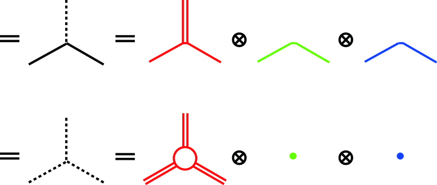
Figure 2: Auxiliary diagrams are depicted for two types of the structure constants, $f_{{\mathfrak{F}}{\mathfrak{F}}{\mathfrak{B}}}\propto\epsilon\gamma\cdot\epsilon\cdot\epsilon$ and $f_{{\mathfrak{B}}{\mathfrak{B}}{\mathfrak{B}}}\propto{\rm Tr}(\gamma\,\gamma\,\gamma)$ with ${\mathfrak{B}}\in\{{\mathfrak{R}},{\mathfrak{L}},{\mathfrak{C}}\}$. Since every structure constant is factorized into three sectors corresponding to three orthogonal $\mathfrak{su}(2)$ subalgebras of $\mathfrak{d}(2,1;\varepsilon)$, we can depict three auxiliary diagrams with three different colors for the original diagram. Here double lines denote indices of the adjoint representation while single lines denote those of the fundamental representation.

Fourthly, we find that the contribution simply vanishes, if $\overline{{\mathfrak{C}}}=\varepsilon{\mathfrak{C}}$ appears in the initial or intermediate states. This can be easily shown by noting the $\varepsilon$-dependence of the structure constants,

$$f_{\overline{{\mathfrak{C}}}}{}^{\overline{{\mathfrak{C}}}\overline{{\mathfrak{C}}}}={\mathcal{O}}(\varepsilon^{1}),\quad f_{\mathfrak{F}}{}^{\overline{{\mathfrak{C}}}{\mathfrak{F}}}={\mathcal{O}}(\varepsilon^{1}),\quad f_{\overline{{\mathfrak{C}}}}{}^{{\mathfrak{F}}{\mathfrak{F}}}={\mathcal{O}}(\varepsilon^{0}),$$

$$f_{\overline{{\mathfrak{C}}}\overline{{\mathfrak{C}}}\overline{{\mathfrak{C}}}}={\mathcal{O}}(\varepsilon^{-1}),\quad f_{\overline{{\mathfrak{C}}}{\mathfrak{F}}{\mathfrak{F}}}={\mathcal{O}}(\varepsilon^{0}).$$ (3.2)

If $\overline{{\mathfrak{C}}}$ appears in the initial or intermediate states, $\overline{{\mathfrak{C}}}$ appears in the superscripts and we have to pick up a factor of $\varepsilon^{1}$ which vanishes in the limit $\varepsilon\to 0$, unless we use the singular structure constant $f_{\overline{{\mathfrak{C}}}\overline{{\mathfrak{C}}}\overline{{\mathfrak{C}}}}={\mathcal{O}}(\varepsilon^{-1})$. If we use the singular structure constant, we need three structure constants with $\overline{{\mathfrak{C}}}$ in the superscripts to contract all the three subscripts, which result in the $\varepsilon$-dependence of $\varepsilon^{-1}\varepsilon^{3}=\varepsilon^{2}$.

Finally, there is a ${\mathbb{Z}}_{2}$ symmetry. If we exchange simultaneously the generators ${\mathfrak{R}}$ and ${\mathfrak{L}}$, the parameters $a^{\mathfrak{a}}$ and $b^{\mathfrak{a}}$ and the states $|\phi\rangle$ and $|\psi\rangle$ (with an appropriate change of signs coming from the parameters $\alpha$ and $\beta$), all the equations remains correct. Namely, it is enough to study half of the relations.

After all these remarks, let us start the computation. In the calculation, it is useful to compute the totally symmetrized generators $\{{\mathfrak{J}}^{L},{\mathfrak{J}}^{M},{\mathfrak{J}}^{N}\}$ first, which we summarize in appendix C. Then, the computation can be easily performed with various formulas of the gamma matrix collected in appendix B.

To summarize the results, we shall introduce here a new notation

$${\mathfrak{J}}^{(A_{1}A_{2}A_{3})}_{\{C_{1}C_{2}C_{3}\}}{\scriptstyle[B_{1}B_{2}B_{3}]}=(-)^{B_{1}(A_{2}+B_{2}+A_{3}+B_{3})+B_{2}(A_{3}+B_{3})}$$

$$\qquad\qquad\qquad\times\{{\mathfrak{J}}^{C_{1}},{\mathfrak{J}}^{C_{2}},{\mathfrak{J}}^{C_{3}}\}f_{C_{1}}{}^{A_{1}B_{1}}f_{C_{2}}{}^{A_{2}B_{2}}f_{C_{3}}{}^{A_{3}B_{3}}f_{B_{1}B_{2}B_{3}}.$$ (3.3)

Hereafter we abbreviate the symbol $|A|$ introduced after (1.1) simply as $A$ when appearing in the exponents of the sign $(-)$ to avoid unnecessary complications.

First, let us concentrate on the case with three bosonic generators in the initial states. Since the initial states do not contain $\overline{{\mathfrak{C}}}$, the initial states can be $({\mathfrak{R}},{\mathfrak{R}},{\mathfrak{R}})$, $({\mathfrak{R}},{\mathfrak{R}},{\mathfrak{L}})$, $({\mathfrak{R}},{\mathfrak{L}},{\mathfrak{L}})$, $({\mathfrak{L}},{\mathfrak{L}},{\mathfrak{L}})$. We start with the case that the initial states are $({\mathfrak{R}},{\mathfrak{R}},{\mathfrak{R}})$. When acting on the bosonic state $|\phi\rangle$, the result vanishes after summing over the cyclic combinations,

$${\mathfrak{J}}^{({\mathfrak{R}}{\mathfrak{R}}{\mathfrak{R}})}_{\{{\mathfrak{R}}{\mathfrak{R}}{\mathfrak{R}}\}}{\scriptstyle[{\mathfrak{R}}{\mathfrak{R}}{\mathfrak{R}}]}|\phi\rangle=0,\quad\bigl{(}{\mathfrak{J}}^{({\mathfrak{R}}{\mathfrak{R}}{\mathfrak{R}})}_{\{{\mathfrak{R}}{\mathfrak{F}}{\mathfrak{F}}\}}{\scriptstyle[{\mathfrak{R}}{\mathfrak{F}}{\mathfrak{F}}]}+{\mathfrak{J}}^{({\mathfrak{R}}{\mathfrak{R}}{\mathfrak{R}})}_{\{{\mathfrak{F}}{\mathfrak{R}}{\mathfrak{F}}\}}{\scriptstyle[{\mathfrak{F}}{\mathfrak{R}}{\mathfrak{F}}]}+{\mathfrak{J}}^{({\mathfrak{R}}{\mathfrak{R}}{\mathfrak{R}})}_{\{{\mathfrak{F}}{\mathfrak{F}}{\mathfrak{R}}\}}{\scriptstyle[{\mathfrak{F}}{\mathfrak{F}}{\mathfrak{R}}]}\bigr{)}|\phi\rangle=0,$$ (3.4)

while when acting on the fermionic state $|\psi\rangle$, each term vanishes independently. Let us turn to the case with the initial states being $({\mathfrak{R}},{\mathfrak{L}},{\mathfrak{L}})$. Similarly, when acting on the bosonic state, the symmetric sum vanishes,

$${\mathfrak{J}}^{({\mathfrak{R}}{\mathfrak{L}}{\mathfrak{L}})}_{\{{\mathfrak{R}}{\mathfrak{F}}{\mathfrak{F}}\}}{\scriptstyle[{\mathfrak{R}}{\mathfrak{F}}{\mathfrak{F}}]}|\phi\rangle=0,\quad\bigl{(}{\mathfrak{J}}^{({\mathfrak{R}}{\mathfrak{L}}{\mathfrak{L}})}_{\{{\mathfrak{F}}{\mathfrak{L}}{\mathfrak{F}}\}}{\scriptstyle[{\mathfrak{F}}{\mathfrak{L}}{\mathfrak{F}}]}+{\mathfrak{J}}^{({\mathfrak{R}}{\mathfrak{L}}{\mathfrak{L}})}_{\{{\mathfrak{F}}{\mathfrak{F}}{\mathfrak{L}}\}}{\scriptstyle[{\mathfrak{F}}{\mathfrak{F}}{\mathfrak{L}}]}\bigr{)}|\phi\rangle=0,$$ (3.5)

while when acting on the fermionic state, each term vanishes separately. The remaining initial states $({\mathfrak{R}},{\mathfrak{R}},{\mathfrak{L}})$ and $({\mathfrak{L}},{\mathfrak{L}},{\mathfrak{L}})$ can also be seen from the above-mentioned ${\mathbb{Z}}_{2}$ symmetry.

Next, let us study the case with two bosonic generators in the initial states. Again due to the absence of $\overline{{\mathfrak{C}}}$ in the initial states, we have only to study three cases with the initial states being $({\mathfrak{R}},{\mathfrak{R}},{\mathfrak{F}})$, $({\mathfrak{R}},{\mathfrak{L}},{\mathfrak{F}})$, $({\mathfrak{L}},{\mathfrak{L}},{\mathfrak{F}})$. Let us start with the case with the initial states being $({\mathfrak{R}},{\mathfrak{R}},{\mathfrak{F}})$. This time, the following combinations vanish on any state $|\chi\rangle$ including the bosonic one or the fermionic one.

$$\bigl{(}{\mathfrak{J}}^{({\mathfrak{R}}{\mathfrak{R}}{\mathfrak{F}})}_{\{{\mathfrak{R}}{\mathfrak{R}}{\mathfrak{F}}\}}{\scriptstyle[{\mathfrak{R}}{\mathfrak{R}}{\mathfrak{R}}]}+{\mathfrak{J}}^{({\mathfrak{R}}{\mathfrak{R}}{\mathfrak{F}})}_{\{{\mathfrak{R}}{\mathfrak{F}}{\mathfrak{R}}\}}{\scriptstyle[{\mathfrak{R}}{\mathfrak{F}}{\mathfrak{F}}]}+{\mathfrak{J}}^{({\mathfrak{R}}{\mathfrak{R}}{\mathfrak{F}})}_{\{{\mathfrak{F}}{\mathfrak{R}}{\mathfrak{R}}\}}{\scriptstyle[{\mathfrak{F}}{\mathfrak{R}}{\mathfrak{F}}]}\bigr{)}|\chi\rangle=0,$$

$$\bigl{(}{\mathfrak{J}}^{({\mathfrak{R}}{\mathfrak{R}}{\mathfrak{F}})}_{\{{\mathfrak{R}}{\mathfrak{F}}{\mathfrak{L}}\}}{\scriptstyle[{\mathfrak{R}}{\mathfrak{F}}{\mathfrak{F}}]}+{\mathfrak{J}}^{({\mathfrak{R}}{\mathfrak{R}}{\mathfrak{F}})}_{\{{\mathfrak{F}}{\mathfrak{R}}{\mathfrak{L}}\}}{\scriptstyle[{\mathfrak{F}}{\mathfrak{R}}{\mathfrak{F}}]}\bigr{)}|\chi\rangle=0,$$

$$\bigl{(}{\mathfrak{J}}^{({\mathfrak{R}}{\mathfrak{R}}{\mathfrak{F}})}_{\{{\mathfrak{R}}{\mathfrak{F}}\overline{{\mathfrak{C}}}\}}{\scriptstyle[{\mathfrak{R}}{\mathfrak{F}}{\mathfrak{F}}]}+{\mathfrak{J}}^{({\mathfrak{R}}{\mathfrak{R}}{\mathfrak{F}})}_{\{{\mathfrak{F}}{\mathfrak{R}}\overline{{\mathfrak{C}}}\}}{\scriptstyle[{\mathfrak{F}}{\mathfrak{R}}{\mathfrak{F}}]}\bigr{)}|\chi\rangle=0,$$

$${\mathfrak{J}}^{({\mathfrak{R}}{\mathfrak{R}}{\mathfrak{F}})}_{\{{\mathfrak{F}}{\mathfrak{F}}{\mathfrak{F}}\}}{\scriptstyle[{\mathfrak{F}}{\mathfrak{F}}{\mathfrak{R}}]}|\chi\rangle=0,\quad{\mathfrak{J}}^{({\mathfrak{R}}{\mathfrak{R}}{\mathfrak{F}})}_{\{{\mathfrak{F}}{\mathfrak{F}}{\mathfrak{F}}\}}{\scriptstyle[{\mathfrak{F}}{\mathfrak{F}}{\mathfrak{L}}]}|\chi\rangle=0.$$ (3.6)

If the initial states are $({\mathfrak{R}},{\mathfrak{L}},{\mathfrak{F}})$, then all the contributions are proportional to a single state with different coefficients. Though it is difficult to specify which combinations of diagrams cancel among themselves, we find it interesting to note that the pairs with ${\mathfrak{R}}$ and ${\mathfrak{L}}$ almost exchanged cancel each other.

$$\bigl{(}{\mathfrak{J}}^{({\mathfrak{R}}{\mathfrak{L}}{\mathfrak{F}})}_{\{{\mathfrak{R}}{\mathfrak{F}}{\mathfrak{R}}\}}{\scriptstyle[{\mathfrak{R}}{\mathfrak{F}}{\mathfrak{F}}]}+{\mathfrak{J}}^{({\mathfrak{R}}{\mathfrak{L}}{\mathfrak{F}})}_{\{{\mathfrak{F}}{\mathfrak{L}}{\mathfrak{L}}\}}{\scriptstyle[{\mathfrak{F}}{\mathfrak{L}}{\mathfrak{F}}]}\bigr{)}|\chi\rangle=0,$$

$$\bigl{(}{\mathfrak{J}}^{({\mathfrak{R}}{\mathfrak{L}}{\mathfrak{F}})}_{\{{\mathfrak{R}}{\mathfrak{F}}{\mathfrak{L}}\}}{\scriptstyle[{\mathfrak{R}}{\mathfrak{F}}{\mathfrak{F}}]}+{\mathfrak{J}}^{({\mathfrak{R}}{\mathfrak{L}}{\mathfrak{F}})}_{\{{\mathfrak{F}}{\mathfrak{L}}{\mathfrak{R}}\}}{\scriptstyle[{\mathfrak{F}}{\mathfrak{L}}{\mathfrak{F}}]}\bigr{)}|\chi\rangle=0,$$

$$\bigl{(}{\mathfrak{J}}^{({\mathfrak{R}}{\mathfrak{L}}{\mathfrak{F}})}_{\{{\mathfrak{R}}{\mathfrak{F}}\overline{{\mathfrak{C}}}\}}{\scriptstyle[{\mathfrak{R}}{\mathfrak{F}}{\mathfrak{F}}]}+{\mathfrak{J}}^{({\mathfrak{R}}{\mathfrak{L}}{\mathfrak{F}})}_{\{{\mathfrak{F}}{\mathfrak{L}}\overline{{\mathfrak{C}}}\}}{\scriptstyle[{\mathfrak{F}}{\mathfrak{L}}{\mathfrak{F}}]}\bigr{)}|\chi\rangle=0,$$

$${\mathfrak{J}}^{({\mathfrak{R}}{\mathfrak{L}}{\mathfrak{F}})}_{\{{\mathfrak{F}}{\mathfrak{F}}{\mathfrak{F}}\}}{\scriptstyle[{\mathfrak{F}}{\mathfrak{F}}{\mathfrak{R}}]}|\chi\rangle=0,\quad{\mathfrak{J}}^{({\mathfrak{R}}{\mathfrak{L}}{\mathfrak{F}})}_{\{{\mathfrak{F}}{\mathfrak{F}}{\mathfrak{F}}\}}{\scriptstyle[{\mathfrak{F}}{\mathfrak{F}}{\mathfrak{L}}]}|\chi\rangle=0.$$ (3.7)

Also, the case with $({\mathfrak{L}},{\mathfrak{L}},{\mathfrak{F}})$ is known from the ${\mathbb{Z}}_{2}$ symmetry.

Subsequently, the next subject is the case with only one bosonic state, namely $({\mathfrak{R}},{\mathfrak{F}},{\mathfrak{F}})$ (with $({\mathfrak{L}},{\mathfrak{F}},{\mathfrak{F}})$ seen from the above ${\mathbb{Z}}_{2}$ symmetry and $(\overline{{\mathfrak{C}}},{\mathfrak{F}},{\mathfrak{F}})$ vanishing by counting the $\varepsilon$-dependence). When acting on the bosonic state, the result is proportional to a single state again. Since it is difficult to explain which combinations cancel among themselves, we shall list up the results.

$$\Bigl{(}{\mathfrak{J}}^{({\mathfrak{R}}{\mathfrak{F}}{\mathfrak{F}})}_{\{{\mathfrak{R}}{\mathfrak{R}}{\mathfrak{R}}\}}{\scriptstyle[{\mathfrak{R}}{\mathfrak{F}}{\mathfrak{F}}]}+[{\mathfrak{J}}^{({\mathfrak{R}}{\mathfrak{F}}{\mathfrak{F}})}_{\{{\mathfrak{R}}{\mathfrak{R}}\overline{{\mathfrak{C}}}\}}{\scriptstyle[{\mathfrak{R}}{\mathfrak{F}}{\mathfrak{F}}]}+\mbox{sym}]+{\mathfrak{J}}^{({\mathfrak{R}}{\mathfrak{F}}{\mathfrak{F}})}_{\{{\mathfrak{R}}\overline{{\mathfrak{C}}}\overline{{\mathfrak{C}}}\}}{\scriptstyle[{\mathfrak{R}}{\mathfrak{F}}{\mathfrak{F}}]}+{\mathfrak{J}}^{({\mathfrak{R}}{\mathfrak{F}}{\mathfrak{F}})}_{\{{\mathfrak{R}}{\mathfrak{F}}{\mathfrak{F}}\}}{\scriptstyle[{\mathfrak{R}}{\mathfrak{R}}{\mathfrak{R}}]}$$

$$+[{\mathfrak{J}}^{({\mathfrak{R}}{\mathfrak{F}}{\mathfrak{F}})}_{\{{\mathfrak{F}}{\mathfrak{R}}{\mathfrak{F}}\}}{\scriptstyle[{\mathfrak{F}}{\mathfrak{F}}{\mathfrak{R}}]}+\mbox{sym}]+[{\mathfrak{J}}^{({\mathfrak{R}}{\mathfrak{F}}{\mathfrak{F}})}_{\{{\mathfrak{F}}{\mathfrak{L}}{\mathfrak{F}}\}}{\scriptstyle[{\mathfrak{F}}{\mathfrak{F}}{\mathfrak{R}}]}+\mbox{sym}]+[{\mathfrak{J}}^{({\mathfrak{R}}{\mathfrak{F}}{\mathfrak{F}})}_{\{{\mathfrak{F}}\overline{{\mathfrak{C}}}{\mathfrak{F}}\}}{\scriptstyle[{\mathfrak{F}}{\mathfrak{F}}{\mathfrak{R}}]}+\mbox{sym}]$$

$$+[{\mathfrak{J}}^{({\mathfrak{R}}{\mathfrak{F}}{\mathfrak{F}})}_{\{{\mathfrak{F}}{\mathfrak{R}}{\mathfrak{F}}\}}{\scriptstyle[{\mathfrak{F}}{\mathfrak{F}}{\mathfrak{L}}]}+\mbox{sym}]+[{\mathfrak{J}}^{({\mathfrak{R}}{\mathfrak{F}}{\mathfrak{F}})}_{\{{\mathfrak{F}}{\mathfrak{L}}{\mathfrak{F}}\}}{\scriptstyle[{\mathfrak{F}}{\mathfrak{F}}{\mathfrak{L}}]}+\mbox{sym}]+[{\mathfrak{J}}^{({\mathfrak{R}}{\mathfrak{F}}{\mathfrak{F}})}_{\{{\mathfrak{F}}\overline{{\mathfrak{C}}}{\mathfrak{F}}\}}{\scriptstyle[{\mathfrak{F}}{\mathfrak{F}}{\mathfrak{L}}]}+\mbox{sym}]\Bigr{)}|\phi^{k}\rangle$$

$$=\Bigl{(}-\frac{5}{4}+0+\frac{3}{4}+1+\frac{1}{4}-\frac{3}{8}-\frac{3}{8}+\frac{3}{4}+\frac{3}{8}-\frac{9}{8}\Bigr{)}\epsilon^{\beta\gamma}\epsilon^{\mathfrak{b}\mathfrak{c}}\Bigl{[}(\gamma^{k}_{l}\gamma^{\boldsymbol{a}}\epsilon)^{bc}+(\gamma^{k}_{l}\gamma^{\boldsymbol{a}}\epsilon)^{cb}\Bigr{]}|\phi^{l}\rangle,$$ (3.8)

where sym denotes the symmetric combination under the exchange between the second particle and the third one in the intermediate and final states and we have specified the indices of the initial states as $({\mathfrak{R}}^{\boldsymbol{a}},{\mathfrak{F}}^{b\beta\mathfrak{b}},{\mathfrak{F}}^{c\gamma\mathfrak{c}})$. When acting on the fermionic state, each symmetric combination in the square parenthesis vanishes separately.

Finally, let us study the case without bosonic generators in the initial state. As in the case of $({\mathfrak{R}},{\mathfrak{L}},{\mathfrak{F}})$ there is a simple rule of the cancellation. We find that the diagrams with ${\mathfrak{R}}$ and ${\mathfrak{L}}$ exchanged cancel each other. Namely, the cancellation happens as follows.

$$\bigl{(}{\mathfrak{J}}^{({\mathfrak{F}}{\mathfrak{F}}{\mathfrak{F}})}_{\{{\mathfrak{R}}{\mathfrak{R}}{\mathfrak{F}}\}}{\scriptstyle[{\mathfrak{F}}{\mathfrak{F}}{\mathfrak{R}}]}+{\mathfrak{J}}^{({\mathfrak{F}}{\mathfrak{F}}{\mathfrak{F}})}_{\{{\mathfrak{L}}{\mathfrak{L}}{\mathfrak{F}}\}}{\scriptstyle[{\mathfrak{F}}{\mathfrak{F}}{\mathfrak{L}}]}+\mbox{cyc}\bigr{)}|\chi\rangle=0,$$

$$\bigl{(}{\mathfrak{J}}^{({\mathfrak{F}}{\mathfrak{F}}{\mathfrak{F}})}_{\{{\mathfrak{R}}{\mathfrak{R}}{\mathfrak{F}}\}}{\scriptstyle[{\mathfrak{F}}{\mathfrak{F}}{\mathfrak{L}}]}+{\mathfrak{J}}^{({\mathfrak{F}}{\mathfrak{F}}{\mathfrak{F}})}_{\{{\mathfrak{L}}{\mathfrak{L}}{\mathfrak{F}}\}}{\scriptstyle[{\mathfrak{F}}{\mathfrak{F}}{\mathfrak{R}}]}+\mbox{cyc}\bigr{)}|\chi\rangle=0,$$

$$\bigl{(}{\mathfrak{J}}^{({\mathfrak{F}}{\mathfrak{F}}{\mathfrak{F}})}_{\{{\mathfrak{R}}{\mathfrak{L}}{\mathfrak{F}}\}}{\scriptstyle[{\mathfrak{F}}{\mathfrak{F}}{\mathfrak{R}}]}+{\mathfrak{J}}^{({\mathfrak{F}}{\mathfrak{F}}{\mathfrak{F}})}_{\{{\mathfrak{R}}{\mathfrak{L}}{\mathfrak{F}}\}}{\scriptstyle[{\mathfrak{F}}{\mathfrak{F}}{\mathfrak{L}}]}+\mbox{tot sym}\bigr{)}|\chi\rangle=0,$$

$$\bigl{(}{\mathfrak{J}}^{({\mathfrak{F}}{\mathfrak{F}}{\mathfrak{F}})}_{\{\overline{{\mathfrak{C}}}\overline{{\mathfrak{C}}}{\mathfrak{F}}\}}{\scriptstyle[{\mathfrak{F}}{\mathfrak{F}}{\mathfrak{R}}]}+{\mathfrak{J}}^{({\mathfrak{F}}{\mathfrak{F}}{\mathfrak{F}})}_{\{\overline{{\mathfrak{C}}}\overline{{\mathfrak{C}}}{\mathfrak{F}}\}}{\scriptstyle[{\mathfrak{F}}{\mathfrak{F}}{\mathfrak{L}}]}+\mbox{cyc}\bigr{)}|\chi\rangle=0,$$

$$\bigl{(}{\mathfrak{J}}^{({\mathfrak{F}}{\mathfrak{F}}{\mathfrak{F}})}_{\{{\mathfrak{R}}\overline{{\mathfrak{C}}}{\mathfrak{F}}\}}{\scriptstyle[{\mathfrak{F}}{\mathfrak{F}}{\mathfrak{R}}]}+{\mathfrak{J}}^{({\mathfrak{F}}{\mathfrak{F}}{\mathfrak{F}})}_{\{{\mathfrak{L}}\overline{{\mathfrak{C}}}{\mathfrak{F}}\}}{\scriptstyle[{\mathfrak{F}}{\mathfrak{F}}{\mathfrak{L}}]}+\mbox{tot sym}\bigr{)}|\chi\rangle=0,$$

$$\bigl{(}{\mathfrak{J}}^{({\mathfrak{F}}{\mathfrak{F}}{\mathfrak{F}})}_{\{{\mathfrak{R}}\overline{{\mathfrak{C}}}{\mathfrak{F}}\}}{\scriptstyle[{\mathfrak{F}}{\mathfrak{F}}{\mathfrak{L}}]}+{\mathfrak{J}}^{({\mathfrak{F}}{\mathfrak{F}}{\mathfrak{F}})}_{\{{\mathfrak{L}}\overline{{\mathfrak{C}}}{\mathfrak{F}}\}}{\scriptstyle[{\mathfrak{F}}{\mathfrak{F}}{\mathfrak{R}}]}+\mbox{tot sym}\bigr{)}|\chi\rangle=0,$$

$$\bigl{(}{\mathfrak{J}}^{({\mathfrak{F}}{\mathfrak{F}}{\mathfrak{F}})}_{\{{\mathfrak{F}}{\mathfrak{F}}{\mathfrak{F}}\}}{\scriptstyle[{\mathfrak{R}}{\mathfrak{R}}{\mathfrak{R}}]}+{\mathfrak{J}}^{({\mathfrak{F}}{\mathfrak{F}}{\mathfrak{F}})}_{\{{\mathfrak{F}}{\mathfrak{F}}{\mathfrak{F}}\}}{\scriptstyle[{\mathfrak{L}}{\mathfrak{L}}{\mathfrak{L}}]}\bigr{)}|\chi\rangle=0,$$ (3.9)

where cyc denotes the summation over the cyclic rotation of three particles in the intermediate and final states and tot sym denotes the totally symmetric summation.

To summarize, we have proved that the right-hand-side of the Serre relation (1.2) vanishes on the representation, which enables the fundamental representation of $\mathfrak{psu}(2|2)\ltimes\mathbb{R}^{3}$ (2.10) to be the evaluation representation for the Yangian algebra.

4 Higher grade generators

As we mentioned in the introduction, the meaning of the Serre relation is to impose constraints on the higher grade generators [12]. Namely, in terms of the BRST charge ${\mathcal{Q}}$, the Serre relation (1.2), stemming from the homomorphism of the coproduct $\Delta\bigl{(}{\mathcal{Q}}\bigl{(}[\widehat{\mathfrak{J}},\widehat{\mathfrak{J}}]\bigr{)}\bigr{)}={\mathcal{Q}}\bigl{(}[\Delta\widehat{\mathfrak{J}},\Delta\widehat{\mathfrak{J}}]\bigr{)}$ (3.1), takes the form ${\mathcal{Q}}\bigl{(}[\widehat{\mathfrak{J}},\widehat{\mathfrak{J}}]\bigr{)}={\mathfrak{J}}^{3}$ schematically, which puts constraints on the commutator of the grade-1 generators $[\widehat{\mathfrak{J}},\widehat{\mathfrak{J}}]$. As we have studied the Serre relation in the previous section, let us now turn to the construction of higher grade generators.

It is natural to expect that the grade-2 generator is generated by the commutator of the grade-1 generators $[\widehat{\mathfrak{J}},\widehat{\mathfrak{J}}]={\mathcal{Q}}\widehat{\widehat{\mathfrak{J}}}+X$, namely,

$$[\widehat{\mathfrak{J}}^{B},\widehat{\mathfrak{J}}^{C}]=\widehat{\widehat{\mathfrak{J}}}{}^{A}f_{A}{}^{BC}+X^{BC}.$$ (4.1)

The inclusion of an extra term $X^{BC}$ is inevitable from the constraint of the Serre relation, which requires $X^{BC}$ to be subject to the condition ${\mathcal{Q}}X={\mathfrak{J}}^{3}$, or explicitly,

$$X^{(A|D}f_{D}{}^{|BC)}=\frac{\hbar^{2}}{24}(-)^{I(B+C)+JC}\{{\mathfrak{J}}^{L},{\mathfrak{J}}^{M},{\mathfrak{J}}^{N}\}f_{L}{}^{AI}f_{M}{}^{BJ}f_{N}{}^{CK}f_{KJI},$$ (4.2)

with the symbol $(A|\cdot|BC)$ in the superscripts denoting summation over the cyclic rotation of $A$, $B$ and $C$ with the suitable Grassmannian charges. Note that there is a gauge ambiguity to shift $X$ and $\widehat{\widehat{{\mathfrak{J}}}}$ simultaneously by $X\to X-{\mathcal{Q}}Y$ and $\widehat{\widehat{{\mathfrak{J}}}}\to\widehat{\widehat{{\mathfrak{J}}}}+Y$.

For the case that the quadratic Casimir operator of the adjoint representation $c_{2}$ (defined by $f_{A}{}^{BC}f_{CBD}=c_{2}g_{AD}$) is non-vanishing, there is a simple choice of the gauge fixing condition ${\mathcal{Q}}^{-1}X=0$, namely, $X^{BC}f_{CB}{}^{A}/c_{2}=0$. In this gauge, we can solve (4.1) for the grade-2 generator and arrive at the canonical definition of it [12],

$$\widehat{\widehat{\mathfrak{J}}}{}^{A}=\frac{1}{c_{2}}[\widehat{\mathfrak{J}}^{B},\widehat{\mathfrak{J}}^{C}]f_{CB}{}^{A},$$ (4.3)

Note that the expression (4.3) is a symmetry of the R-matrix and the normalization is compatible with the evaluation representation ${\mathfrak{J}}^{A}_{n}\simeq(iu)^{n}{\mathfrak{J}}^{A}$. By plugging the coproduct of the grade-1 generator

$$\Delta\widehat{\mathfrak{J}}^{A}=\widehat{\mathfrak{J}}^{A}\otimes 1+1\otimes\widehat{\mathfrak{J}}^{A}+\frac{\hbar}{2}{\mathfrak{J}}^{M}\otimes{\mathfrak{J}}^{N}f_{NM}{}^{A},$$ (4.4)

into the expression of the grade-2 generator (4.3), the coproduct of the grade-2 generator is found to be

$$\Delta\widehat{\widehat{\mathfrak{J}}}{}^{A}=\widehat{\widehat{\mathfrak{J}}}{}^{A}\otimes 1+1\otimes\widehat{\widehat{\mathfrak{J}}}{}^{A}+\frac{\hbar}{2}\bigl{(}\widehat{\mathfrak{J}}^{M}\otimes{\mathfrak{J}}^{N}+{\mathfrak{J}}^{M}\otimes\widehat{\mathfrak{J}}^{N}\bigr{)}f_{NM}{}^{A}$$

$$\quad-\frac{\hbar^{2}}{8c_{2}}(-)^{IC}\bigl{(}\{{\mathfrak{J}}^{L},{\mathfrak{J}}^{M}\}\otimes{\mathfrak{J}}^{N}+(-)^{N(L+M)}{\mathfrak{J}}^{N}\otimes\{{\mathfrak{J}}^{L},{\mathfrak{J}}^{M}\}\bigr{)}f_{L}{}^{BI}f_{M}{}^{CJ}f_{NJI}f_{CB}{}^{A}.$$ (4.5)

Note that the results (4.3) and (4.5) rely heavily on the fact that the quadratic Casimir operator $c_{2}$ is non-vanishing. However, for the superalgebra we are considering now it is not difficult to show $c_{2}=0$ even for the $\varepsilon$-deformed exceptional superalgebra $\mathfrak{d}(2,1;\varepsilon)$. In this case, we have to take another suitable gauge fixing condition. To respect the compatibility of the evaluation representation in (4.1), the extra term $X^{BC}$ must be vanishing on all states. Therefore, it is natural to choose a gauge so that

$$X^{BC}|\chi\rangle=0.$$ (4.6)

Then the problem is reduced to find an expression of $X^{BC}$ which satisfies the Serre relation (4.2) and the above gauge condition (4.6) simultaneously. A naive candidate coming from the derivation of the Serre relation in appendix A is (See e.g. (A.2).)

$$\widetilde{X}^{BC}=-\frac{1}{3}\cdot\frac{\hbar^{2}}{24}(-)^{IC}\{{\mathfrak{J}}^{L},{\mathfrak{J}}^{M},{\mathfrak{J}}^{N}\}f_{L}{}^{BI}f_{M}{}^{CJ}f_{NJI}.$$ (4.7)

As the computation in appendix A, using the Jacobi identity twice, we can show that this expression $\widetilde{X}^{BC}$ is a solution to (4.2). However, this is not compatible with the condition (4.6). Actually, using the formulas summarized in appendices B and C, it is not difficult to show that $\widetilde{X}^{BC}$ takes the following form on the fundamental representation of $\mathfrak{psu}(2|2)\ltimes\mathbb{R}^{3}$,

$$\widetilde{X}^{BC}|\chi\rangle=-2\cdot\frac{\hbar^{2}}{24}[{\mathfrak{J}}^{B},{\mathfrak{J}}^{C}]|\chi\rangle.$$ (4.8)

In order to satisfy the condition (4.6), we can improve $\widetilde{X}$ without violating the Serre relation (4.2) by subtracting the commutator since it is a ${\mathcal{Q}}$-exact term, or schematically $\widetilde{X}\to\widetilde{X}-{\mathcal{Q}}Y$. Finally we adopt the following expression for $X^{BC}$,

$$X^{BC}=-\frac{1}{3}\cdot\frac{\hbar^{2}}{24}\Bigl{(}(-)^{IC}\{{\mathfrak{J}}^{L},{\mathfrak{J}}^{M},{\mathfrak{J}}^{N}\}f_{L}{}^{BI}f_{M}{}^{CJ}f_{NJI}-6{\mathfrak{J}}^{A}f_{A}{}^{BC}\Bigr{)}.$$ (4.9)

Note that the relation (4.8) is interesting by itself. As mentioned above, $\widetilde{X}^{(A|D}f_{D}{}^{|BC)}$ (or ${\mathcal{Q}}\widetilde{X}$) is equal to the right-hand-side of the Serre relation (1.2) at the algebraic level. Since (4.8) indicates that $\widetilde{X}$ is ${\mathcal{Q}}$-exact on the representation, this gives an alternative proof of the compatibility of the evaluation representation with the Serre relation, which has been directly proved in section 3. This argument will be important in the next section.

As the final project of this section, let us construct the coproduct of the grade-2 generator by requiring the homomorphism of the coproduct for the grade-1 commutator $\Delta\bigl{(}[\widehat{\mathfrak{J}}^{A},\widehat{\mathfrak{J}}^{B}]\bigr{)}=[\Delta\widehat{\mathfrak{J}}{}^{A},\Delta\widehat{\mathfrak{J}}{}^{B}]$. Using the commutator of the grade-1 generators as in (4.1), we can write down the coproduct coupled with the structure constant as,

$$\Delta\widehat{\widehat{\mathfrak{J}}}{}^{A}f_{A}{}^{BC}=[\Delta\widehat{\mathfrak{J}}^{B},\Delta\widehat{\mathfrak{J}}^{C}]-\Delta X^{BC}.$$ (4.10)

The reader may worry that the quadratic Casimir operator $c_{2}$ may appear again on the left-hand-side when we solve for the grade-2 generator $\Delta\widehat{\widehat{\mathfrak{J}}}{}^{A}$. However, this is not the case. Because it can be shown that the right-hand-side is also proportional to the structure constants $f_{A}{}^{BC}$, we find a solution of the grade-2 generator just by dropping the same structure constants. More precisely, the vanishing of $c_{2}$ in the superalgebra $\mathfrak{d}(2,1;\varepsilon)$ (and its limiting case $\mathfrak{psu}(2|2)\ltimes{\mathbb{R}}^{3})$ is a consequence of summing over all the bosonic and fermionic intermediate generators $B$ and $C$ in $f_{A}{}^{BC}f_{CBD}=c_{2}g_{AD}$. However, if we fix the intermediate generators and sum only over all the indices of the generators, the result is proportional to the Killing form $g_{AD}$ with a non-vanishing coefficient,

$$f_{{\mathfrak{R}}^{\boldsymbol{a}}}{}^{{\mathfrak{R}}^{\boldsymbol{b}}{\mathfrak{R}}^{\boldsymbol{c}}}f_{{\mathfrak{R}}^{\boldsymbol{c}}{\mathfrak{R}}^{\boldsymbol{b}}{\mathfrak{R}}^{\boldsymbol{d}}} =-4\alpha g_{{\mathfrak{R}}^{\boldsymbol{a}}{\mathfrak{R}}^{\boldsymbol{d}}}, f_{{\mathfrak{R}}^{\boldsymbol{a}}}{}^{{\mathfrak{F}}^{B}{\mathfrak{F}}^{C}}f_{{\mathfrak{F}}^{C}{\mathfrak{F}}^{B}{\mathfrak{R}}^{\boldsymbol{d}}} =4\alpha g_{{\mathfrak{R}}^{\boldsymbol{a}}{\mathfrak{R}}^{\boldsymbol{d}}}, f_{{\mathfrak{F}}^{A}}{}^{{\mathfrak{R}}^{\boldsymbol{b}}{\mathfrak{F}}^{C}}f_{{\mathfrak{F}}^{C}{\mathfrak{R}}^{\boldsymbol{b}}{\mathfrak{F}}^{D}} =-\frac{3}{2}\alpha g_{{\mathfrak{F}}^{A}{\mathfrak{F}}^{D}},$$

$$f_{{\mathfrak{L}}^{\boldsymbol{\alpha}}}{}^{{\mathfrak{L}}^{\boldsymbol{\beta}}{\mathfrak{L}}^{\boldsymbol{\gamma}}}f_{{\mathfrak{L}}^{\boldsymbol{\gamma}}{\mathfrak{L}}^{\boldsymbol{\beta}}{\mathfrak{L}}^{\boldsymbol{\delta}}} =-4\beta g_{{\mathfrak{L}}^{\boldsymbol{\alpha}}{\mathfrak{L}}^{\boldsymbol{\delta}}}, f_{{\mathfrak{L}}^{\boldsymbol{\alpha}}}{}^{{\mathfrak{F}}^{B}{\mathfrak{F}}^{C}}f_{{\mathfrak{F}}^{C}{\mathfrak{F}}^{B}{\mathfrak{L}}^{\boldsymbol{\delta}}} =4\beta g_{{\mathfrak{L}}^{\boldsymbol{\alpha}}{\mathfrak{L}}^{\boldsymbol{\delta}}}, f_{{\mathfrak{F}}^{A}}{}^{{\mathfrak{L}}^{\boldsymbol{\beta}}{\mathfrak{F}}^{C}}f_{{\mathfrak{F}}^{C}{\mathfrak{L}}^{\boldsymbol{\beta}}{\mathfrak{F}}^{D}} =-\frac{3}{2}\beta g_{{\mathfrak{F}}^{A}{\mathfrak{F}}^{D}},$$

$$f_{{\mathfrak{C}}^{\boldsymbol{\mathfrak{a}}}}{}^{{\mathfrak{C}}^{\boldsymbol{\mathfrak{b}}}{\mathfrak{C}}^{\boldsymbol{\mathfrak{c}}}}f_{{\mathfrak{C}}^{\boldsymbol{\mathfrak{c}}}{\mathfrak{C}}^{\boldsymbol{\mathfrak{b}}}{\mathfrak{C}}^{\boldsymbol{\mathfrak{d}}}} =-4\gamma g_{{\mathfrak{C}}^{\boldsymbol{\mathfrak{a}}}{\mathfrak{C}}^{\boldsymbol{\mathfrak{d}}}}, f_{{\mathfrak{C}}^{\boldsymbol{\mathfrak{a}}}}{}^{{\mathfrak{F}}^{B}{\mathfrak{F}}^{C}}f_{{\mathfrak{F}}^{C}{\mathfrak{F}}^{B}{\mathfrak{C}}^{\boldsymbol{\mathfrak{d}}}} =4\gamma g_{{\mathfrak{C}}^{\boldsymbol{\mathfrak{a}}}{\mathfrak{C}}^{\boldsymbol{\mathfrak{d}}}}, f_{{\mathfrak{F}}^{A}}{}^{{\mathfrak{C}}^{\boldsymbol{\mathfrak{b}}}{\mathfrak{F}}^{C}}f_{{\mathfrak{F}}^{C}{\mathfrak{C}}^{\boldsymbol{\mathfrak{b}}}{\mathfrak{F}}^{D}} =-\frac{3}{2}\gamma g_{{\mathfrak{F}}^{A}{\mathfrak{F}}^{D}},$$ (4.11)

where we have introduced the capital Latin letter $A$ temporally to represent all of the fermionic indices $(a,\alpha,\mathfrak{a})$ for the notational simplicity. The Killing form of the bosonic generators is proportional to the metric $g_{{\mathfrak{R}}^{\boldsymbol{a}}{\mathfrak{R}}^{\boldsymbol{b}}}=-\alpha g_{\boldsymbol{a}\boldsymbol{b}}$, $g_{{\mathfrak{L}}^{\boldsymbol{\alpha}}{\mathfrak{L}}^{\boldsymbol{\beta}}}=-\beta g_{\boldsymbol{\alpha}\boldsymbol{\beta}}$, $g_{{\mathfrak{C}}^{\boldsymbol{\mathfrak{a}}}{\mathfrak{C}}^{\boldsymbol{\mathfrak{b}}}}=-\gamma g_{\boldsymbol{\mathfrak{a}}\boldsymbol{\mathfrak{b}}}$, while that of the fermionic ones are $g_{{\mathfrak{F}}^{A}{\mathfrak{F}}^{B}}=\epsilon_{ab}\epsilon_{\alpha\beta}\epsilon_{\mathfrak{a}\mathfrak{b}}$. Therefore, when the right-hand-side of (4.10) is proportional to the structure constant $f_{A}{}^{BC}$, we can restrict the intermediate generators $B$ and $C$ to specific generators and obtain the grade-2 generator without using the quadratic Casimir operator $c_{2}$.

After all, the explicit form of the coproduct is

$$\Delta\widehat{\widehat{\mathfrak{J}}}{}^{A}=\widehat{\widehat{\mathfrak{J}}}{}^{A}\otimes 1+1\otimes\widehat{\widehat{\mathfrak{J}}}{}^{A}+\frac{\hbar}{2}\bigl{(}\widehat{\mathfrak{J}}^{M}\otimes{\mathfrak{J}}^{N}+{\mathfrak{J}}^{M}\otimes\widehat{\mathfrak{J}}^{N}\bigr{)}f_{NM}{}^{A}$$

$$\qquad\quad-\frac{\hbar^{2}}{24}\bigl{(}\{{\mathfrak{J}}^{L},{\mathfrak{J}}^{M}\}\otimes{\mathfrak{J}}^{N}+(-)^{N(L+M)}{\mathfrak{J}}^{N}\otimes\{{\mathfrak{J}}^{L},{\mathfrak{J}}^{M}\}\bigr{)}f_{L}{}^{AI}f_{MNI},$$ (4.12)

which is obviously the symmetry of the R-matrix by the construction (4.10) and valid even if $c_{2}=0$.

5 Lift to exceptional superalgebra

In our discussion of the higher grade generators in the previous section, we have found a simple expression (4.2) for the right-hand-side of the Serre relation in terms of $\widetilde{X}^{BC}$ (4.7). Namely, the compatibility of the evaluation representation reduces to the equation

$$\widetilde{X}^{(A|D}f_{D}{}^{|BC)}|\chi\rangle=0,$$ (5.1)

when acting on the representation. For the previous case of $\mathfrak{psu}(2|2)\ltimes{\mathbb{R}}^{3}$, it is surprising to find that actually (4.8) holds. Then, the compatibility (5.1) is automatic from the nilpotency of the BRST charge ${\mathcal{Q}}$ (or the Jacobi identity). In this simplified expression, it is not difficult to find that the above argument is still valid for the case of the exceptional superalgebra $\mathfrak{d}(2,1;\varepsilon)$. Namely, using the formulas in appendix D for $\mathfrak{d}(2,1;\varepsilon)$, after some computation we find a relation which is a natural lift of (4.8),

$$\widetilde{X}^{BC}|\chi\rangle=2\alpha\beta\cdot\frac{\hbar^{2}}{24}[{\mathfrak{J}}^{B},{\mathfrak{J}}^{C}]|\chi\rangle,$$ (5.2)

where the indices $B$ and $C$ run over all generators including ${\mathfrak{C}}^{\boldsymbol{\mathfrak{a}}}$. This final result implies that the infinite-dimensional representation of $\mathfrak{d}(2,1;\varepsilon)$ (2.8) is also extended to the evaluation representation of the Yangian algebra. Since the expression is parallel to the case of $\mathfrak{psu}(2|2)\ltimes{\mathbb{R}}^{3}$, the higher grade generators can be constructed similarly as in the previous section.

6 Discussion

We have proved that the evaluation representation adopted in the AdS/CFT spin chain model is compatible with the Serre relation of the Yangian algebra for both the cases of $\mathfrak{psu}(2|2)\ltimes{\mathbb{R}}^{3}$ and $\mathfrak{d}(2,1;\varepsilon)$. Conceptually, the Serre relation imposes constraints on higher grade generators. Therefore, it is inevitable to prove the Serre relation in order to proceed to the infinite symmetry of string theory. Technically, we have introduced a new formalism for the algebra and the representation via the three-dimensional gamma matrix. We have also found that the generator $\widetilde{X}^{BC}$ coming from later discussions on higher grade generators is useful to simplify the proof. We believe that our formulation can further apply to many related computations as well. For example, the determination of the R-matrix for the fundamental excitations [8, 23] and the bound states [10] should be done in a much simpler way using our gamma matrix formulation.

We also analyze the higher grade generators, where we find that the argument and the formula become subtle and singular because the quadratic Casimir operator of the adjoint representation $c_{2}$ is vanishing. Here by changing the gauge fixing condition we propose an alternative non-singular construction of the higher grade generator which is a symmetry of the R-matrix and at the same time compatible with the evaluation representation.

Let us list several further directions to conclude this paper.

As we have suggested in the introduction, the compatibility of the evaluation representation may indicate a close relation to the string worldsheet theory. The fact that the evaluation representation is lifted to the exceptional superalgebra $\mathfrak{d}(2,1;\varepsilon)$ may imply its string interpretation. We would like to pursue this possibility further in our future work.

In our simplified proof, we introduce a generator $\widetilde{X}^{BC}$ and find that it is proportional to the commutator $[{\mathfrak{J}}^{B},{\mathfrak{J}}^{C}]$ on the representation. Since it can be seen directly from the definition (4.7) that $\widetilde{X}{}^{BC}$ is antisymmetric (in the generalized sense) and the result has to transform canonically as the product of ${\mathfrak{J}}^{B}$ and ${\mathfrak{J}}^{C}$, it is not surprising to find the proportionality. What is surprising is that all of the results come with the same proportionality constant. Our understanding would be clearer if we can rewrite the proportionality constant $-2$ and $2\alpha\beta$ in (4.8) and (5.2) in the terminology of the representation theory. The value of the quadratic Casimir operator for $\mathfrak{d}(2,1;\varepsilon)$, ${\mathcal{T}}^{\mathfrak{d}}|\chi\rangle=(\alpha\beta/4\gamma)|\chi\rangle$ would be a clue.

A topic related to our motivation of constructing higher grade generators is the universal R-matrix [24, 17], where the Chevalley-Serre basis is conventionally adopted. It would be great to find the universal R-matrix both for $\mathfrak{psu}(2|2)\ltimes{\mathbb{R}}^{3}$ and $\mathfrak{d}(2,1;\varepsilon)$, which contains all of the higher grade generators.

An interesting proposal that the conventional and dual superconformal symmetries form the Yangian algebra together was made very recently [25], where the vanishing Casimir operator $c_{2}=0$ plays an important role in the consistency. We would like to understand the relation to our present discussion.

Since the interacting theory of string theory is not so different from the free theory locally on the worldsheet and since the correspondence between gauge theory and string theory works well also at the interacting level [26, 27], it would be interesting to study the integrability at the interacting level more extensively and define interacting string theory with Yang-Mills theory.

Appendix A Homomorphism of coproduct

In this appendix we would like to explain that the origin of the Serre relation stems from the homomorphism of the coproduct of the grade-1 generators defined in (4.4). The result in this appendix is well-known and also appears previously in, for example, [12, 19]. The reason we recapitulate it here is because of the possible sign ambiguity in dealing with the superalgebra. In sections 3-5 we have found many cancellations and simplifications, which do not happen if we take the wrong signs.

Let us start with computing $[\Delta\widehat{\mathfrak{J}}^{A},[\Delta\widehat{\mathfrak{J}}^{B},\Delta{\mathfrak{J}}^{C}]]=[\Delta\widehat{\mathfrak{J}}^{A},\Delta\widehat{\mathfrak{J}}^{J}f_{J}{}^{BC}]$. From the expression

$$[{\mathfrak{J}}^{P}\otimes{\mathfrak{J}}^{Q},{\mathfrak{J}}^{R}\otimes{\mathfrak{J}}^{S}]=\frac{1}{2}(-)^{QR}\bigl{(}[{\mathfrak{J}}^{P},{\mathfrak{J}}^{R}]\otimes\{{\mathfrak{J}}^{Q},{\mathfrak{J}}^{S}\}+\{{\mathfrak{J}}^{P},{\mathfrak{J}}^{R}\}\otimes[{\mathfrak{J}}^{Q},{\mathfrak{J}}^{S}]\bigr{)},$$ (A.1)

we find that the terms with only Lie algebra generators are given as

$$[\Delta\widehat{\mathfrak{J}}^{A},[\Delta\widehat{\mathfrak{J}}^{B},\Delta{\mathfrak{J}}^{C}]]\Big{|}_{{\rm Lie}} =\frac{\hbar^{2}}{8}(-)^{IL+IM+KM}f_{LI}{}^{A}f_{MK}{}^{J}f_{N}{}^{IK}f_{J}{}^{BC}$$

$$\quad\times\bigl{(}\{{\mathfrak{J}}^{L},{\mathfrak{J}}^{M}\}\otimes{\mathfrak{J}}^{N}+(-)^{N(L+M)}{\mathfrak{J}}^{N}\otimes\{{\mathfrak{J}}^{L},{\mathfrak{J}}^{M}\}\bigr{)}.$$ (A.2)

Here the signs can be interpreted as the Grassmannian charges when we contract the superscripts with the subscripts in the canonical position of the spinor indices as in (1.2). We can continue the computations keeping the above interpretation of the signs systematically. For this purpose, we have to introduce an extra sign $(-)^{(P+Q)(R+S+T)}$, even if we simply commute ${\mathfrak{J}}^{N}f_{N}{}^{PQ}$ with the bosonic structure constants $f^{RST}$. Further, using twice the Jacobi identity

$$f_{MK}{}^{J}f_{J}{}^{BC} =-(-)^{K(B+C)}f_{M}{}^{BJ}f_{J}{}^{C}{}_{K}-(-)^{C(K+B)}f_{M}{}^{CJ}f_{JK}{}^{B},$$

$$f_{NI}{}^{K}f_{KJ}{}^{C} =-(-)^{C(I+J)}f_{N}{}^{CK}f_{KIJ}-(-)^{I(J+C)}f_{NJ}{}^{K}f_{K}{}^{C}{}_{I},$$ (A.3)

and noting $\{{\mathfrak{J}}^{L},{\mathfrak{J}}^{M}\}f_{L}{}^{AI}f_{M}{}^{CJ}=(-)^{(A+I)(C+J)}\{{\mathfrak{J}}^{L},{\mathfrak{J}}^{M}\}f_{L}{}^{CJ}f_{M}{}^{AI}$, finally we arrive at the expression

$$[\Delta\widehat{\mathfrak{J}}^{A},[\Delta\widehat{\mathfrak{J}}^{B},\Delta{\mathfrak{J}}^{C}]]\Big{|}_{{\rm Lie}}=\frac{\hbar^{2}}{8}\bigl{(}\{{\mathfrak{J}}^{L},{\mathfrak{J}}^{M}\}\otimes{\mathfrak{J}}^{N}+(-)^{N(L+M)}{\mathfrak{J}}^{N}\otimes\{{\mathfrak{J}}^{L},{\mathfrak{J}}^{M}\}\bigr{)}$$

$$\quad\times\bigl{(}(-)^{JC+I(B+C)}f_{L}{}^{AI}f_{M}{}^{BJ}f_{N}{}^{CK}f_{KJI}$$

$$\qquad+(-)^{IB}f_{L}{}^{AI}f_{M}{}^{BJ}f_{NJ}{}^{K}f_{KI}{}^{C}-(-)^{IA+C(A+B)}f_{L}{}^{CI}f_{M}{}^{AJ}f_{NJ}{}^{K}f_{KI}{}^{B}\bigr{)}.$$ (A.4)

Adding the terms coming from the cyclic rotation of $(A,B,C)$, the second term and the third term cancel each other while the first term becomes totally symmetric in the indices $L,M,N$. The final form indicates that the mapping of coproduct $\Delta$ is homomorphic with respect to the bracket product (3.1) if the Serre relation holds.

Appendix B Useful formulas of gamma matrices

Here we collect some of the formulas of the gamma matrices. First using the definition of the gamma matrices (2.4), we can show the following ones without difficulty.

$$(\gamma^{\boldsymbol{A}}\gamma_{\boldsymbol{A}})^{K}{}_{L}=3\delta^{K}_{L},\quad(\gamma^{\boldsymbol{B}}\gamma^{\boldsymbol{A}}\gamma_{\boldsymbol{B}})^{K}{}_{L}=-(\gamma^{\boldsymbol{A}})^{K}{}_{L},\quad(\gamma^{\boldsymbol{C}}\gamma^{\boldsymbol{A}}\gamma^{\boldsymbol{B}}\gamma_{\boldsymbol{C}})^{K}{}_{L}=(\gamma^{\boldsymbol{A}}\gamma^{\boldsymbol{B}}+2\gamma^{\boldsymbol{B}}\gamma^{\boldsymbol{A}})^{K}{}_{L},$$

$${\rm Tr}(\gamma^{\boldsymbol{A}}\gamma^{\boldsymbol{B}})=2g^{\boldsymbol{A}\boldsymbol{B}},\quad{\rm Tr}(\gamma^{\boldsymbol{A}}\gamma^{\boldsymbol{B}}\gamma^{\boldsymbol{C}}\gamma^{\boldsymbol{D}})=2(g^{\boldsymbol{A}\boldsymbol{B}}g^{\boldsymbol{C}\boldsymbol{D}}-g^{\boldsymbol{A}\boldsymbol{C}}g^{\boldsymbol{B}\boldsymbol{D}}+g^{\boldsymbol{A}\boldsymbol{D}}g^{\boldsymbol{B}\boldsymbol{C}}).$$ (B.1)

If we further combine the use of the Fierz identity

$$(\gamma^{\boldsymbol{A}})^{K}{}_{L}(\gamma_{\boldsymbol{A}})^{M}{}_{N}=2\delta^{K}_{N}\delta^{M}_{L}-\delta^{K}_{L}\delta^{M}_{N}=-\sqrt{2}(\gamma^{K}_{L})^{M}{}_{N},$$ (B.2)

we also find that

$${\rm Tr}(\gamma^{\boldsymbol{A}}\gamma^{\boldsymbol{B}}\gamma^{\boldsymbol{C}})(\gamma_{\boldsymbol{C}})^{K}{}_{L}=2((\gamma^{\boldsymbol{A}}\gamma^{\boldsymbol{B}})^{K}{}_{L}-\delta^{K}_{L}g^{\boldsymbol{A}\boldsymbol{B}}),$$

$${\rm Tr}(\gamma^{\boldsymbol{A}}\gamma^{\boldsymbol{B}}\gamma^{\boldsymbol{E}}){\rm Tr}(\gamma^{\boldsymbol{C}}\gamma^{\boldsymbol{D}}\gamma_{\boldsymbol{E}})=4(-g^{\boldsymbol{A}\boldsymbol{C}}g^{\boldsymbol{B}\boldsymbol{D}}+g^{\boldsymbol{A}\boldsymbol{D}}g^{\boldsymbol{B}\boldsymbol{C}}).$$ (B.3)

Note that the last formula is nothing but the famous one $\epsilon_{\boldsymbol{A}\boldsymbol{B}\boldsymbol{E}}\epsilon_{\boldsymbol{C}\boldsymbol{D}\boldsymbol{E}}=\delta_{\boldsymbol{A}\boldsymbol{C}}\delta_{\boldsymbol{B}\boldsymbol{D}}-\delta_{\boldsymbol{A}\boldsymbol{D}}\delta_{\boldsymbol{B}\boldsymbol{C}}$ for $\boldsymbol{A},\boldsymbol{B},\cdots=1,2,3$.

Appendix C Totally symmetrized generators

It is useful here to summarize the action of various totally symmetrized generators $\{{\mathfrak{J}}^{A},{\mathfrak{J}}^{B},{\mathfrak{J}}^{C}\}$ appearing in the computation. We classify the formulas into four cases depending on whether the totally symmetrized generators and the states are bosonic or fermionic.

$\bullet\;\{$bosonic$\}|\phi\rangle$

$$\{{\mathfrak{R}}^{\boldsymbol{a}},{\mathfrak{R}}^{\boldsymbol{b}},{\mathfrak{R}}^{\boldsymbol{c}}\}|\phi^{k}\rangle=-\frac{1}{\sqrt{2}}(g^{\boldsymbol{b}\boldsymbol{c}}\gamma^{\boldsymbol{a}}+g^{\boldsymbol{c}\boldsymbol{a}}\gamma^{\boldsymbol{b}}+g^{\boldsymbol{a}\boldsymbol{b}}\gamma^{\boldsymbol{c}})^{k}{}_{l}|\phi^{l}\rangle,$$

$$\{{\mathfrak{R}}^{\boldsymbol{a}},{\mathfrak{R}}^{\boldsymbol{b}},\overline{{\mathfrak{C}}}{}^{\boldsymbol{\mathfrak{c}}}\}|\phi^{k}\rangle=3\overline{C}{}^{\boldsymbol{\mathfrak{c}}}g^{\boldsymbol{a}\boldsymbol{b}}|\phi^{k}\rangle,\quad\{{\mathfrak{R}}^{\boldsymbol{a}},\overline{{\mathfrak{C}}}{}^{\boldsymbol{\mathfrak{b}}},\overline{{\mathfrak{C}}}{}^{\boldsymbol{\mathfrak{c}}}\}|\phi^{k}\rangle=-3\sqrt{2}\overline{C}^{\boldsymbol{\mathfrak{b}}}\overline{C}^{\boldsymbol{\mathfrak{c}}}(\gamma^{\boldsymbol{a}})^{k}{}_{l}|\phi^{l}\rangle,$$

$$\{{\mathfrak{R}}^{\boldsymbol{a}},{\mathfrak{F}}^{b\beta\mathfrak{b}},{\mathfrak{F}}^{c\gamma\mathfrak{c}}\}|\phi^{k}\rangle=-\epsilon^{\beta\gamma}\Bigl{[}(\gamma^{\boldsymbol{a}}\epsilon)^{bc}\delta^{k}_{l}(\overline{{C\!\!\!\!/\,}}\epsilon)^{\mathfrak{b}\mathfrak{c}}+\frac{1}{\sqrt{2}}\epsilon^{bc}(\gamma^{\boldsymbol{a}})^{k}{}_{l}\epsilon^{\mathfrak{b}\mathfrak{c}}\Bigr{]}|\phi^{l}\rangle,$$

$$\{{\mathfrak{L}}^{\boldsymbol{\alpha}},{\mathfrak{F}}^{b\beta\mathfrak{b}},{\mathfrak{F}}^{c\gamma\mathfrak{c}}\}|\phi^{k}\rangle=\frac{1}{2}(\gamma^{\boldsymbol{\alpha}}\epsilon)^{\beta\gamma}\Bigl{[}\epsilon^{bc}\delta^{k}_{l}(\overline{{C\!\!\!\!/\,}}\epsilon)^{\mathfrak{b}\mathfrak{c}}-(\gamma^{k}_{l}\epsilon)^{bc}\epsilon^{\mathfrak{b}\mathfrak{c}}\Bigr{]}|\phi^{l}\rangle,$$

$$\{\overline{{\mathfrak{C}}}{}^{\boldsymbol{\mathfrak{a}}},{\mathfrak{F}}^{b\beta\mathfrak{b}},{\mathfrak{F}}^{c\gamma\mathfrak{c}}\}|\phi^{k}\rangle=-\frac{3}{2}\overline{C}{}^{\boldsymbol{\mathfrak{a}}}\epsilon^{\beta\gamma}\Bigl{[}2(\gamma^{k}_{l}\epsilon)^{bc}(\overline{{C\!\!\!\!/\,}}\epsilon)^{\mathfrak{b}\mathfrak{c}}-\epsilon^{bc}\delta^{k}_{l}\epsilon^{\mathfrak{b}\mathfrak{c}}\Bigr{]}|\phi^{l}\rangle.$$ (C.1)

$\bullet\;\{$bosonic$\}|\psi\rangle$

$$\{{\mathfrak{L}}^{\boldsymbol{\alpha}},{\mathfrak{L}}^{\boldsymbol{\beta}},{\mathfrak{L}}^{\boldsymbol{\gamma}}\}|\psi^{\kappa}\rangle=-\frac{1}{\sqrt{2}}(g^{\boldsymbol{\beta}\boldsymbol{\gamma}}\gamma^{\boldsymbol{\alpha}}+g^{\boldsymbol{\gamma}\boldsymbol{\alpha}}\gamma^{\boldsymbol{\beta}}+g^{\boldsymbol{\alpha}\boldsymbol{\beta}}\gamma^{\boldsymbol{\gamma}})^{\kappa}{}_{\lambda}|\psi^{\lambda}\rangle,$$

$$\{{\mathfrak{L}}^{\boldsymbol{\alpha}},{\mathfrak{L}}^{\boldsymbol{\beta}},\overline{{\mathfrak{C}}}{}^{\boldsymbol{\mathfrak{c}}}\}|\psi^{\kappa}\rangle=3\overline{C}{}^{\boldsymbol{\mathfrak{c}}}g^{\boldsymbol{\alpha}\boldsymbol{\beta}}|\psi^{\kappa}\rangle,\quad\{{\mathfrak{L}}^{\boldsymbol{\alpha}},\overline{{\mathfrak{C}}}{}^{\boldsymbol{\mathfrak{b}}},\overline{{\mathfrak{C}}}{}^{\boldsymbol{\mathfrak{c}}}\}|\psi^{\kappa}\rangle=-3\sqrt{2}\overline{C}{}^{\boldsymbol{\mathfrak{b}}}\overline{C}{}^{\boldsymbol{\mathfrak{c}}}(\gamma^{\boldsymbol{\alpha}})^{\kappa}{}_{\lambda}|\psi^{\lambda}\rangle,$$

$$\{{\mathfrak{R}}^{\boldsymbol{a}},{\mathfrak{F}}^{b\beta\mathfrak{b}},{\mathfrak{F}}^{c\gamma\mathfrak{c}}\}|\psi^{\kappa}\rangle=\frac{1}{2}(\gamma^{\boldsymbol{a}}\epsilon)^{bc}\Bigl{[}\epsilon^{\beta\gamma}\delta^{\kappa}_{\lambda}(\overline{{C\!\!\!\!/\,}}\epsilon)^{\mathfrak{b}\mathfrak{c}}+(\gamma^{\kappa}_{\lambda}\epsilon)^{\beta\gamma}\epsilon^{\mathfrak{b}\mathfrak{c}}\Bigr{]}|\psi^{\lambda}\rangle,$$

$$\{{\mathfrak{L}}^{\boldsymbol{\alpha}},{\mathfrak{F}}^{b\beta\mathfrak{b}},{\mathfrak{F}}^{c\gamma\mathfrak{c}}\}|\psi^{\kappa}\rangle=-\epsilon^{bc}\Bigl{[}(\gamma^{\boldsymbol{\alpha}}\epsilon)^{\beta\gamma}\delta^{\kappa}_{\lambda}(\overline{{C\!\!\!\!/\,}}\epsilon)^{\mathfrak{b}\mathfrak{c}}-\frac{1}{\sqrt{2}}\epsilon^{\beta\gamma}(\gamma^{\boldsymbol{\alpha}})^{\kappa}{}_{\lambda}\epsilon^{\mathfrak{b}\mathfrak{c}}\Bigr{]}|\psi^{\lambda}\rangle,$$

$$\{\overline{{\mathfrak{C}}}{}^{\boldsymbol{\mathfrak{a}}},{\mathfrak{F}}^{b\beta\mathfrak{b}},{\mathfrak{F}}^{c\gamma\mathfrak{c}}\}|\psi^{\kappa}\rangle=-\frac{3}{2}\overline{C}{}^{\boldsymbol{\mathfrak{a}}}\epsilon^{bc}\Bigl{[}2(\gamma^{\kappa}_{\lambda}\epsilon)^{\beta\gamma}(\overline{{C\!\!\!\!/\,}}\epsilon)^{\mathfrak{b}\mathfrak{c}}+\epsilon^{\beta\gamma}\delta^{\kappa}_{\lambda}\epsilon^{\mathfrak{b}\mathfrak{c}}\Bigr{]}|\psi^{\lambda}\rangle.$$ (C.2)

$\bullet\;\{$fermionic$\}|\phi\rangle$

$$\{{\mathfrak{R}}^{\boldsymbol{a}},{\mathfrak{R}}^{\boldsymbol{b}},{\mathfrak{F}}^{c\gamma\mathfrak{c}}\}|\phi^{k}\rangle=-a^{\mathfrak{c}}g^{\boldsymbol{a}\boldsymbol{b}}\epsilon^{kc}|\psi^{\gamma}\rangle,\quad\{{\mathfrak{R}}^{\boldsymbol{a}},\overline{{\mathfrak{C}}}{}^{\boldsymbol{\mathfrak{b}}},{\mathfrak{F}}^{c\gamma\mathfrak{c}}\}|\phi^{k}\rangle=\frac{3}{\sqrt{2}}\overline{C}{}^{\boldsymbol{\mathfrak{b}}}a^{\mathfrak{c}}(\gamma^{\boldsymbol{a}}\epsilon)^{kc}|\psi^{\gamma}\rangle,$$

$$\{{\mathfrak{L}}^{\boldsymbol{\alpha}},{\mathfrak{L}}^{\boldsymbol{\beta}},{\mathfrak{F}}^{c\gamma\mathfrak{c}}\}|\phi^{k}\rangle=-a^{\mathfrak{c}}\epsilon^{kc}g^{\boldsymbol{\alpha}\boldsymbol{\beta}}|\psi^{\gamma}\rangle,\quad\{{\mathfrak{L}}^{\boldsymbol{\alpha}},\overline{{\mathfrak{C}}}{}^{\boldsymbol{\mathfrak{b}}},{\mathfrak{F}}^{c\gamma\mathfrak{c}}\}|\phi^{k}\rangle=\frac{3}{\sqrt{2}}\overline{C}{}^{\boldsymbol{\mathfrak{b}}}a^{\mathfrak{c}}\epsilon^{kc}(\gamma^{\boldsymbol{\alpha}})^{\gamma}{}_{\lambda}|\psi^{\lambda}\rangle,$$

$$\{{\mathfrak{R}}^{\boldsymbol{a}},{\mathfrak{L}}^{\boldsymbol{\beta}},{\mathfrak{F}}^{c\gamma\mathfrak{c}}\}|\phi^{k}\rangle=-\frac{1}{2}a^{\mathfrak{c}}(\gamma^{\boldsymbol{a}}\epsilon)^{kc}(\gamma^{\boldsymbol{\beta}})^{\gamma}{}_{\lambda}|\psi^{\lambda}\rangle,\quad\{\overline{{\mathfrak{C}}}{}^{\boldsymbol{\mathfrak{a}}},\overline{{\mathfrak{C}}}{}^{\boldsymbol{\mathfrak{b}}},{\mathfrak{F}}^{c\gamma\mathfrak{c}}\}|\phi^{k}\rangle=-6\overline{C}{}^{\boldsymbol{\mathfrak{a}}}\overline{C}{}^{\boldsymbol{\mathfrak{b}}}a^{\mathfrak{c}}\epsilon^{kc}|\psi^{\gamma}\rangle,$$

$$\{{\mathfrak{F}}^{a\alpha\mathfrak{a}},{\mathfrak{F}}^{b\beta\mathfrak{b}},{\mathfrak{F}}^{c\gamma\mathfrak{c}}\}|\phi^{k}\rangle=\bigl{(}b^{\mathfrak{a}}a^{\mathfrak{b}}a^{\mathfrak{c}}+b^{\mathfrak{b}}a^{\mathfrak{c}}a^{\mathfrak{a}}+b^{\mathfrak{c}}a^{\mathfrak{a}}a^{\mathfrak{b}}\bigr{)}\epsilon^{kl}\bigl{(}\epsilon^{bc}\delta^{a}_{l}\epsilon^{\gamma\alpha}\delta^{\beta}_{\lambda}-\epsilon^{ca}\delta^{b}_{l}\epsilon^{\beta\gamma}\delta^{\alpha}_{\lambda}\bigr{)}|\psi^{\lambda}\rangle.$$ (C.3)

$\bullet\;\{$fermionic$\}|\psi\rangle$

$$\{{\mathfrak{R}}^{\boldsymbol{a}},{\mathfrak{R}}^{\boldsymbol{b}},{\mathfrak{F}}^{c\gamma\mathfrak{c}}\}|\psi^{\kappa}\rangle=b^{\mathfrak{c}}g^{\boldsymbol{a}\boldsymbol{b}}\epsilon^{\kappa\gamma}|\phi^{c}\rangle,\quad\{{\mathfrak{R}}^{\boldsymbol{a}},\overline{{\mathfrak{C}}}{}^{\boldsymbol{\mathfrak{b}}},{\mathfrak{F}}^{c\gamma\mathfrak{c}}\}|\psi^{\kappa}\rangle=-\frac{3}{\sqrt{2}}\overline{C}{}^{\boldsymbol{\mathfrak{b}}}b^{\mathfrak{c}}\epsilon^{\kappa\gamma}(\gamma^{\boldsymbol{a}})^{c}{}_{l}|\phi^{l}\rangle,$$

$$\{{\mathfrak{L}}^{\boldsymbol{\alpha}},{\mathfrak{L}}^{\boldsymbol{\beta}},{\mathfrak{F}}^{c\gamma\mathfrak{c}}\}|\psi^{\kappa}\rangle=b^{\mathfrak{c}}\epsilon^{\kappa\gamma}g^{\boldsymbol{\alpha}\boldsymbol{\beta}}|\phi^{c}\rangle,\quad\{{\mathfrak{L}}^{\boldsymbol{\alpha}},\overline{{\mathfrak{C}}}{}^{\boldsymbol{\mathfrak{b}}},{\mathfrak{F}}^{c\gamma\mathfrak{c}}\}|\psi^{\kappa}\rangle=-\frac{3}{\sqrt{2}}\overline{C}{}^{\boldsymbol{\mathfrak{b}}}b^{\mathfrak{c}}(\gamma^{\boldsymbol{\alpha}}\epsilon)^{\kappa\gamma}|\phi^{c}\rangle,$$

$$\{{\mathfrak{R}}^{\boldsymbol{a}},{\mathfrak{L}}^{\boldsymbol{\beta}},{\mathfrak{F}}^{c\gamma\mathfrak{c}}\}|\psi^{\kappa}\rangle=\frac{1}{2}b^{\mathfrak{c}}(\gamma^{\boldsymbol{a}})^{c}{}_{l}(\gamma^{\boldsymbol{\beta}}\epsilon)^{\kappa\gamma}|\phi^{l}\rangle,\quad\{\overline{{\mathfrak{C}}}{}^{\boldsymbol{\mathfrak{a}}},\overline{{\mathfrak{C}}}{}^{\boldsymbol{\mathfrak{b}}},{\mathfrak{F}}^{c\gamma\mathfrak{c}}\}|\psi^{\kappa}\rangle=6\overline{C}{}^{\boldsymbol{\mathfrak{a}}}\overline{C}{}^{\boldsymbol{\mathfrak{b}}}b^{\mathfrak{c}}\epsilon^{\kappa\gamma}|\phi^{c}\rangle,$$

$$\{{\mathfrak{F}}^{a\alpha\mathfrak{a}},{\mathfrak{F}}^{b\beta\mathfrak{b}},{\mathfrak{F}}^{c\gamma\mathfrak{c}}\}|\psi^{\kappa}\rangle=\bigl{(}a^{\mathfrak{a}}b^{\mathfrak{b}}b^{\mathfrak{c}}+a^{\mathfrak{b}}b^{\mathfrak{c}}b^{\mathfrak{a}}+a^{\mathfrak{c}}b^{\mathfrak{a}}b^{\mathfrak{b}}\bigr{)}\epsilon^{\kappa\lambda}\bigl{(}\epsilon^{bc}\delta^{a}_{l}\epsilon^{\gamma\alpha}\delta^{\beta}_{\lambda}-\epsilon^{ca}\delta^{b}_{l}\epsilon^{\beta\gamma}\delta^{\alpha}_{\lambda}\bigr{)}|\phi^{l}\rangle.$$ (C.4)

Note that the combination $\epsilon^{bc}\delta^{a}_{l}\epsilon^{\gamma\alpha}\delta^{\beta}_{\lambda}-\epsilon^{ca}\delta^{b}_{l}\epsilon^{\beta\gamma}\delta^{\alpha}_{\lambda}$ in the right-hand-side of the last lines in (C.3) and (C.4) does not seem to respect the totally symmetric property of the left-hand-side at the first sight. However, there is an interesting cyclic property in this combination,

$$\epsilon^{bc}\delta^{a}_{l}\epsilon^{\gamma\alpha}\delta^{\beta}_{\lambda}-\epsilon^{ca}\delta^{b}_{l}\epsilon^{\beta\gamma}\delta^{\alpha}_{\lambda}=\epsilon^{ca}\delta^{b}_{l}\epsilon^{\alpha\beta}\delta^{\gamma}_{\lambda}-\epsilon^{ab}\delta^{c}_{l}\epsilon^{\gamma\alpha}\delta^{\beta}_{\lambda}=\epsilon^{ab}\delta^{c}_{l}\epsilon^{\beta\gamma}\delta^{\alpha}_{\lambda}-\epsilon^{bc}\delta^{a}_{l}\epsilon^{\alpha\beta}\delta^{\gamma}_{\lambda},$$ (C.5)

which can be easily proved from $\epsilon^{bc}\delta^{a}_{l}+\epsilon^{ca}\delta^{b}_{l}+\epsilon^{ab}\delta^{c}_{l}=0$ and $\epsilon^{\beta\gamma}\delta^{\alpha}_{\lambda}+\epsilon^{\gamma\alpha}\delta^{\beta}_{\lambda}+\epsilon^{\alpha\beta}\delta^{\gamma}_{\lambda}=0$.

Appendix D Formulas for exceptional superalgebra

In this appendix we shall see how the expression of the totally symmetrized generators of $\mathfrak{psu}(2|2)\ltimes{\mathbb{R}}^{3}$ in the previous appendix is lifted to the case of the exceptional superalgebra $\mathfrak{d}(2,1;\varepsilon)$. Our strategy is to search for a product of the generators which looks simpler but has the same action as the totally symmetrized generators. A naive guess is to rewrite the gamma matrices $\gamma^{k}{}_{l}$ and $\gamma^{\kappa}{}_{\lambda}$ in (C.1)-(C.4) into generators ${\mathfrak{R}}$ and ${\mathfrak{L}}$, and the coefficients $a$, $b$ and $C$ into generators ${\mathfrak{F}}$ and ${\mathfrak{C}}$. Since the the generators do not commute with each other in general, we have to take care of the ordering carefully. Here for simplicity we shall abbreviate the indices of the states as $|\phi\rangle=|\phi^{k}_{m}\rangle$, $|\psi\rangle=|\psi^{\kappa}_{r}\rangle$, because the formulas do not depend on the indices.

$\bullet\;\{$bosonic$\}|\phi\rangle$

$$\{{\mathfrak{R}}^{\boldsymbol{a}},{\mathfrak{R}}^{\boldsymbol{b}},{\mathfrak{R}}^{\boldsymbol{c}}\}|\phi\rangle=(g^{\boldsymbol{b}\boldsymbol{c}}{\mathfrak{R}}^{\boldsymbol{a}}+g^{\boldsymbol{c}\boldsymbol{a}}{\mathfrak{R}}^{\boldsymbol{b}}+g^{\boldsymbol{a}\boldsymbol{b}}{\mathfrak{R}}^{\boldsymbol{c}})|\phi\rangle,$$

$$\{{\mathfrak{R}}^{\boldsymbol{a}},{\mathfrak{R}}^{\boldsymbol{b}},{\mathfrak{C}}{}^{\boldsymbol{\mathfrak{c}}}\}|\phi\rangle=3{\mathfrak{C}}^{\boldsymbol{\mathfrak{c}}}g^{\boldsymbol{a}\boldsymbol{b}}|\phi\rangle,\quad\{{\mathfrak{R}}^{\boldsymbol{a}},{\mathfrak{C}}{}^{\boldsymbol{\mathfrak{b}}},{\mathfrak{C}}{}^{\boldsymbol{\mathfrak{c}}}\}|\phi\rangle=3{\mathfrak{R}}^{\boldsymbol{a}}\{{\mathfrak{C}}{}^{\boldsymbol{\mathfrak{b}}},{\mathfrak{C}}{}^{\boldsymbol{\mathfrak{c}}}\}|\phi\rangle,$$

$$\{{\mathfrak{R}}^{\boldsymbol{a}},{\mathfrak{F}}^{b\beta\mathfrak{b}},{\mathfrak{F}}^{c\gamma\mathfrak{c}}\}|\phi\rangle=-\epsilon^{\beta\gamma}\Bigl{[}\alpha\epsilon^{bc}\epsilon^{\mathfrak{b}\mathfrak{c}}{\mathfrak{R}}^{\boldsymbol{a}}+\gamma(\gamma^{\boldsymbol{a}}\epsilon)^{bc}({\mathfrak{C}}\!\!\!/\epsilon)^{\mathfrak{b}\mathfrak{c}}\Bigr{]}|\phi\rangle,$$

$$\{{\mathfrak{L}}^{\boldsymbol{\alpha}},{\mathfrak{F}}^{b\beta\mathfrak{b}},{\mathfrak{F}}^{c\gamma\mathfrak{c}}\}|\phi\rangle=\frac{1}{2}(\gamma^{\boldsymbol{\alpha}}\epsilon)^{\beta\gamma}\Bigl{[}\alpha({\mathfrak{R}}\!\!\!\!/\,\epsilon)^{bc}\epsilon^{\mathfrak{b}\mathfrak{c}}+\gamma\epsilon^{bc}({\mathfrak{C}}\!\!\!/\epsilon)^{\mathfrak{b}\mathfrak{c}}\Bigr{]}|\phi\rangle,$$

$$\{{\mathfrak{C}}{}^{\boldsymbol{\mathfrak{a}}},{\mathfrak{F}}^{b\beta\mathfrak{b}},{\mathfrak{F}}^{c\gamma\mathfrak{c}}\}|\phi\rangle=\frac{-1}{2}\epsilon^{\beta\gamma}\Bigl{[}({\mathfrak{R}}\!\!\!\!/\,\epsilon)^{bc}\bigl{(}3\gamma\{{\mathfrak{C}}^{\mathfrak{a}},({\mathfrak{C}}\!\!\!/\epsilon)^{\mathfrak{bc}}\}-\alpha(\gamma^{\boldsymbol{\mathfrak{a}}}\epsilon)^{\mathfrak{bc}}\bigr{)}+(3\alpha-\gamma)\epsilon^{bc}\epsilon^{\mathfrak{bc}}{\mathfrak{C}}^{\boldsymbol{\mathfrak{a}}}\Bigr{]}|\phi\rangle.$$ (D.1)

$\bullet\;\{$bosonic$\}|\psi\rangle$

$$\{{\mathfrak{L}}^{\boldsymbol{\alpha}},{\mathfrak{L}}^{\boldsymbol{\beta}},{\mathfrak{L}}^{\boldsymbol{\gamma}}\}|\psi\rangle=(g^{\boldsymbol{\beta}\boldsymbol{\gamma}}{\mathfrak{L}}^{\boldsymbol{\alpha}}+g^{\boldsymbol{\gamma}\boldsymbol{\alpha}}{\mathfrak{L}}^{\boldsymbol{\beta}}+g^{\boldsymbol{\alpha}\boldsymbol{\beta}}{\mathfrak{L}}^{\boldsymbol{\gamma}})|\psi\rangle,$$

$$\{{\mathfrak{L}}^{\boldsymbol{\alpha}},{\mathfrak{L}}^{\boldsymbol{\beta}},{\mathfrak{C}}^{\boldsymbol{\mathfrak{c}}}\}|\psi\rangle=3{\mathfrak{C}}^{\boldsymbol{\mathfrak{c}}}g^{\boldsymbol{\alpha}\boldsymbol{\beta}}|\psi\rangle,\quad\{{\mathfrak{L}}^{\boldsymbol{\alpha}},{\mathfrak{C}}^{\boldsymbol{\mathfrak{b}}},{\mathfrak{C}}^{\boldsymbol{\mathfrak{c}}}\}|\psi\rangle=3{\mathfrak{L}}^{\boldsymbol{\alpha}}\{{\mathfrak{C}}^{\boldsymbol{\mathfrak{b}}},{\mathfrak{C}}^{\boldsymbol{\mathfrak{c}}}\}|\psi\rangle,$$

$$\{{\mathfrak{R}}^{\boldsymbol{a}},{\mathfrak{F}}^{b\beta\mathfrak{b}},{\mathfrak{F}}^{c\gamma\mathfrak{c}}\}|\psi\rangle=\frac{1}{2}(\gamma^{\boldsymbol{a}}\epsilon)^{bc}\Bigl{[}\beta({\mathfrak{L}}\!\!\!/\epsilon)^{\beta\gamma}\epsilon^{\mathfrak{bc}}+\gamma\epsilon^{\beta\gamma}({\mathfrak{C}}\!\!\!/\epsilon)^{\mathfrak{bc}}\Bigr{]}|\psi\rangle,$$

$$\{{\mathfrak{L}}^{\boldsymbol{\alpha}},{\mathfrak{F}}^{b\beta\mathfrak{b}},{\mathfrak{F}}^{c\gamma\mathfrak{c}}\}|\psi\rangle=-\epsilon^{bc}\Bigl{[}\beta\epsilon^{\beta\gamma}\epsilon^{\mathfrak{bc}}{\mathfrak{L}}^{\boldsymbol{\alpha}}+\gamma(\gamma^{\boldsymbol{\alpha}}\epsilon)^{\beta\gamma}({\mathfrak{C}}\!\!\!/\epsilon)^{\mathfrak{bc}}\Bigr{]}|\psi\rangle,$$

$$\{{\mathfrak{C}}^{\boldsymbol{\mathfrak{a}}},{\mathfrak{F}}^{b\beta\mathfrak{b}},{\mathfrak{F}}^{c\gamma\mathfrak{c}}\}|\psi\rangle=\frac{-1}{2}\epsilon^{bc}\Bigl{[}({\mathfrak{L}}\!\!\!/\epsilon)^{\beta\gamma}\bigl{(}3\gamma\{{\mathfrak{C}}^{\mathfrak{a}},({\mathfrak{C}}\!\!\!/\epsilon)^{\mathfrak{bc}}\}-\beta(\gamma^{\boldsymbol{\mathfrak{a}}}\epsilon)^{\mathfrak{bc}}\bigr{)}+(3\beta-\gamma)\epsilon^{\beta\gamma}\epsilon^{\mathfrak{bc}}{\mathfrak{C}}^{\boldsymbol{\mathfrak{a}}}\Bigr{]}|\psi\rangle.$$ (D.2)

$\bullet\;\{$fermionic$\}|\phi\rangle$

$$\{{\mathfrak{R}}^{\boldsymbol{a}},{\mathfrak{R}}^{\boldsymbol{b}},{\mathfrak{F}}^{c\gamma\mathfrak{c}}\}|\phi\rangle=g^{\boldsymbol{a}\boldsymbol{b}}{\mathfrak{F}}^{c\gamma\mathfrak{c}}|\phi\rangle,\quad\{{\mathfrak{R}}^{\boldsymbol{a}},{\mathfrak{C}}^{\boldsymbol{\mathfrak{b}}},{\mathfrak{F}}^{c\gamma\mathfrak{c}}\}|\phi\rangle=\frac{1}{\sqrt{2}}(\gamma^{\boldsymbol{a}})^{c}{}_{d}\Bigl{[}2{\mathfrak{F}}^{d\gamma\mathfrak{c}}{\mathfrak{C}}^{\boldsymbol{\mathfrak{b}}}+{\mathfrak{C}}^{\boldsymbol{\mathfrak{b}}}{\mathfrak{F}}^{d\gamma\mathfrak{c}}\Bigr{]}|\phi\rangle,$$

$$\{{\mathfrak{L}}^{\boldsymbol{\alpha}},{\mathfrak{L}}^{\boldsymbol{\beta}},{\mathfrak{F}}^{c\gamma\mathfrak{c}}\}|\phi\rangle=g^{\boldsymbol{\alpha}\boldsymbol{\beta}}{\mathfrak{F}}^{c\gamma\mathfrak{c}}|\phi\rangle,\quad\{{\mathfrak{L}}^{\boldsymbol{\alpha}},{\mathfrak{C}}^{\boldsymbol{\mathfrak{b}}},{\mathfrak{F}}^{c\gamma\mathfrak{c}}\}|\phi\rangle=\frac{-1}{\sqrt{2}}(\gamma^{\boldsymbol{\alpha}})^{\gamma}{}_{\delta}\Bigr{[}2{\mathfrak{C}}^{\boldsymbol{\mathfrak{b}}}{\mathfrak{F}}^{c\delta\mathfrak{c}}+{\mathfrak{F}}^{c\delta\mathfrak{c}}{\mathfrak{C}}^{\boldsymbol{\mathfrak{b}}}\Bigr{]}|\phi\rangle,$$

$$\{{\mathfrak{R}}^{\boldsymbol{a}},{\mathfrak{L}}^{\boldsymbol{\beta}},{\mathfrak{F}}^{c\gamma\mathfrak{c}}\}|\phi\rangle=\frac{-1}{2}(\gamma^{\boldsymbol{a}})^{c}{}_{d}(\gamma^{\boldsymbol{\beta}})^{\gamma}{}_{\delta}{\mathfrak{F}}^{d\delta\mathfrak{c}}|\phi\rangle,$$

$$\{{\mathfrak{C}}^{\boldsymbol{\mathfrak{a}}},{\mathfrak{C}}^{\boldsymbol{\mathfrak{b}}},{\mathfrak{F}}^{c\gamma\mathfrak{c}}\}|\phi\rangle=\frac{1}{2}\Bigl{[}3\{\{{\mathfrak{C}}^{\boldsymbol{\mathfrak{a}}},{\mathfrak{C}}^{\boldsymbol{\mathfrak{b}}}\},{\mathfrak{F}}^{c\gamma\mathfrak{c}}\}-g^{\boldsymbol{\mathfrak{a}}\boldsymbol{\mathfrak{b}}}{\mathfrak{F}}^{c\gamma\mathfrak{c}}\Bigr{]}|\phi\rangle,$$

$$\{{\mathfrak{F}}^{a\alpha\mathfrak{a}},{\mathfrak{F}}^{b\beta\mathfrak{b}},{\mathfrak{F}}^{c\gamma\mathfrak{c}}\}|\phi\rangle=\frac{-1}{2}\Bigl{\{}3\gamma\Bigl{[}{\mathfrak{F}}^{c\gamma\mathfrak{c}}({\mathfrak{R}}\!\!\!\!/\,\epsilon)^{ab}\epsilon^{\alpha\beta}({\mathfrak{C}}\!\!\!/\epsilon)^{\mathfrak{a}\mathfrak{b}}+\epsilon^{ab}({\mathfrak{L}}\!\!\!/\epsilon)^{\alpha\beta}({\mathfrak{C}}\!\!\!/\epsilon)^{\mathfrak{a}\mathfrak{b}}{\mathfrak{F}}^{c\gamma\mathfrak{c}}-\frac{1}{2}\epsilon^{ab}\epsilon^{\alpha\beta}\epsilon^{\mathfrak{a}\mathfrak{b}}{\mathfrak{F}}^{c\gamma\mathfrak{c}}\Bigr{]}$$

$$\quad+\Bigl{[}\alpha\delta^{c}_{d}\epsilon^{ab}(\gamma^{\gamma}_{\delta}\epsilon)^{\alpha\beta}(\gamma^{\mathfrak{c}}_{\mathfrak{d}}\epsilon)^{\mathfrak{a}\mathfrak{b}}+\beta(\gamma^{c}_{d}\epsilon)^{ab}\delta^{\gamma}_{\delta}\epsilon^{\alpha\beta}(\gamma^{\mathfrak{c}}_{\mathfrak{d}}\epsilon)^{\mathfrak{a}\mathfrak{b}}+\gamma(\gamma^{c}_{d}\epsilon)^{ab}(\gamma^{\gamma}_{\delta}\epsilon)^{\alpha\beta}\delta^{\mathfrak{c}}_{\mathfrak{d}}\epsilon^{\mathfrak{a}\mathfrak{b}}\Bigr{]}{\mathfrak{F}}^{d\delta\mathfrak{d}}\Bigr{\}}|\phi\rangle.$$ (D.3)

$\bullet\;\{$fermionic$\}|\psi\rangle$

$$\{{\mathfrak{R}}^{\boldsymbol{a}},{\mathfrak{R}}^{\boldsymbol{b}},{\mathfrak{F}}^{c\gamma\mathfrak{c}}\}|\psi\rangle=g^{\boldsymbol{a}\boldsymbol{b}}{\mathfrak{F}}^{c\gamma\mathfrak{c}}|\psi\rangle,\quad\{{\mathfrak{R}}^{\boldsymbol{a}},{\mathfrak{C}}^{\boldsymbol{\mathfrak{b}}},{\mathfrak{F}}^{c\gamma\mathfrak{c}}\}|\psi\rangle=\frac{-1}{\sqrt{2}}(\gamma^{\boldsymbol{a}})^{c}{}_{d}\Bigl{[}2{\mathfrak{C}}^{\boldsymbol{\mathfrak{b}}}{\mathfrak{F}}^{d\gamma\mathfrak{c}}+{\mathfrak{F}}^{d\gamma\mathfrak{c}}{\mathfrak{C}}^{\boldsymbol{\mathfrak{b}}}\Bigr{]}|\psi\rangle,$$

$$\{{\mathfrak{L}}^{\boldsymbol{\alpha}},{\mathfrak{L}}^{\boldsymbol{\beta}},{\mathfrak{F}}^{c\gamma\mathfrak{c}}\}|\psi\rangle=g^{\boldsymbol{\alpha}\boldsymbol{\beta}}{\mathfrak{F}}^{c\gamma\mathfrak{c}}|\psi\rangle,\quad\{{\mathfrak{L}}^{\boldsymbol{\alpha}},{\mathfrak{C}}^{\boldsymbol{\mathfrak{b}}},{\mathfrak{F}}^{c\gamma\mathfrak{c}}\}|\psi\rangle=\frac{1}{\sqrt{2}}(\gamma^{\boldsymbol{\alpha}})^{\gamma}{}_{\delta}\Bigr{[}2{\mathfrak{F}}^{c\delta\mathfrak{c}}{\mathfrak{C}}^{\boldsymbol{\mathfrak{b}}}+{\mathfrak{C}}^{\boldsymbol{\mathfrak{b}}}{\mathfrak{F}}^{c\delta\mathfrak{c}}\Bigr{]}|\psi\rangle,$$

$$\{{\mathfrak{R}}^{\boldsymbol{a}},{\mathfrak{L}}^{\boldsymbol{\beta}},{\mathfrak{F}}^{c\gamma\mathfrak{c}}\}|\psi\rangle=\frac{-1}{2}(\gamma^{\boldsymbol{a}})^{c}{}_{d}(\gamma^{\boldsymbol{\beta}})^{\gamma}{}_{\delta}{\mathfrak{F}}^{d\delta\mathfrak{c}}|\psi\rangle,$$

$$\{{\mathfrak{C}}^{\boldsymbol{\mathfrak{a}}},{\mathfrak{C}}^{\boldsymbol{\mathfrak{b}}},{\mathfrak{F}}^{c\gamma\mathfrak{c}}\}|\psi\rangle=\frac{1}{2}\Bigl{[}3\{\{{\mathfrak{C}}^{\boldsymbol{\mathfrak{a}}},{\mathfrak{C}}^{\boldsymbol{\mathfrak{b}}}\},{\mathfrak{F}}^{c\gamma\mathfrak{c}}\}-g^{\boldsymbol{\mathfrak{a}}\boldsymbol{\mathfrak{b}}}{\mathfrak{F}}^{c\gamma\mathfrak{c}}\Bigr{]}|\psi\rangle,$$

$$\{{\mathfrak{F}}^{a\alpha\mathfrak{a}},{\mathfrak{F}}^{b\beta\mathfrak{b}},{\mathfrak{F}}^{c\gamma\mathfrak{c}}\}|\psi\rangle=\frac{-1}{2}\Bigl{\{}3\gamma\Bigl{[}({\mathfrak{R}}\!\!\!\!/\,\epsilon)^{ab}\epsilon^{\alpha\beta}({\mathfrak{C}}\!\!\!/\epsilon)^{\mathfrak{a}\mathfrak{b}}{\mathfrak{F}}^{c\gamma\mathfrak{c}}+{\mathfrak{F}}^{c\gamma\mathfrak{c}}\epsilon^{ab}({\mathfrak{L}}\!\!\!/\epsilon)^{\alpha\beta}({\mathfrak{C}}\!\!\!/\epsilon)^{\mathfrak{a}\mathfrak{b}}-\frac{1}{2}\epsilon^{ab}\epsilon^{\alpha\beta}\epsilon^{\mathfrak{a}\mathfrak{b}}{\mathfrak{F}}^{c\gamma\mathfrak{c}}\Bigr{]}$$

$$\quad+\Bigl{[}\alpha\delta^{c}_{d}\epsilon^{ab}(\gamma^{\gamma}_{\delta}\epsilon)^{\alpha\beta}(\gamma^{\mathfrak{c}}_{\mathfrak{d}}\epsilon)^{\mathfrak{a}\mathfrak{b}}+\beta(\gamma^{c}_{d}\epsilon)^{ab}\delta^{\gamma}_{\delta}\epsilon^{\alpha\beta}(\gamma^{\mathfrak{c}}_{\mathfrak{d}}\epsilon)^{\mathfrak{a}\mathfrak{b}}+\gamma(\gamma^{c}_{d}\epsilon)^{ab}(\gamma^{\gamma}_{\delta}\epsilon)^{\alpha\beta}\delta^{\mathfrak{c}}_{\mathfrak{d}}\epsilon^{\mathfrak{a}\mathfrak{b}}\Bigr{]}{\mathfrak{F}}^{d\delta\mathfrak{d}}\Bigr{\}}|\psi\rangle.$$ (D.4)

In deriving all these expressions the formulas we need are

$$\{{\mathfrak{J}}^{A},{\mathfrak{J}}^{B},{\mathfrak{J}}^{C}\}=\frac{3}{2}\{\{{\mathfrak{J}}^{A},{\mathfrak{J}}^{B}\},{\mathfrak{J}}^{C}\}+\frac{1}{2}(-)^{BC}\Bigl{(}[{\mathfrak{J}}^{A},[{\mathfrak{J}}^{C},{\mathfrak{J}}^{B}]]+[[{\mathfrak{J}}^{A},{\mathfrak{J}}^{C}],{\mathfrak{J}}^{B}]\Bigr{)},$$

$$\{{\mathfrak{R}}^{\boldsymbol{a}},{\mathfrak{R}}^{\boldsymbol{b}}\}|\phi\rangle=g^{\boldsymbol{a}\boldsymbol{b}}|\phi\rangle,\quad\{{\mathfrak{L}}^{\boldsymbol{\alpha}},{\mathfrak{L}}^{\boldsymbol{\beta}}\}|\psi\rangle=g^{\boldsymbol{\alpha}\boldsymbol{\beta}}|\psi\rangle,$$

$$\{{\mathfrak{F}}^{b\beta\mathfrak{b}},{\mathfrak{F}}^{c\gamma\mathfrak{c}}\}|\phi\rangle=-\epsilon^{\beta\gamma}\bigl{[}\gamma({\mathfrak{R}}\!\!\!\!/\,\epsilon)^{bc}({\mathfrak{C}}\!\!\!/\epsilon)^{\mathfrak{b}\mathfrak{c}}+\frac{\alpha}{2}\epsilon^{bc}\epsilon^{\mathfrak{b}\mathfrak{c}}\bigr{]}|\phi\rangle,$$

$$\{{\mathfrak{F}}^{b\beta\mathfrak{b}},{\mathfrak{F}}^{c\gamma\mathfrak{c}}\}|\psi\rangle=-\epsilon^{bc}\bigl{[}\gamma({\mathfrak{L}}\!\!\!/\epsilon)^{\beta\gamma}({\mathfrak{C}}\!\!\!/\epsilon)^{\mathfrak{b}\mathfrak{c}}+\frac{\beta}{2}\epsilon^{\beta\gamma}\epsilon^{\mathfrak{b}\mathfrak{c}}\bigr{]}|\psi\rangle,$$ (D.5)

while the following formulas

$${\mathfrak{C}}^{\boldsymbol{\mathfrak{a}}}{\mathfrak{C}}_{\boldsymbol{\mathfrak{a}}}|\phi\rangle=\frac{-1}{2\gamma^{2}}(2\alpha\beta+\alpha^{2})|\phi\rangle,\quad{\mathfrak{C}}^{\boldsymbol{\mathfrak{a}}}{\mathfrak{C}}_{\boldsymbol{\mathfrak{a}}}|\psi\rangle=\frac{-1}{2\gamma^{2}}(2\alpha\beta+\beta^{2})|\psi\rangle,$$

$${\mathfrak{F}}^{a\alpha\mathfrak{a}}({\mathfrak{C}}\!\!\!/)^{\mathfrak{b}}{}_{\mathfrak{a}}|\phi\rangle=-\frac{\alpha+2\beta}{\sqrt{2}\gamma}{\mathfrak{F}}^{a\alpha\mathfrak{b}}|\phi\rangle,\quad({\mathfrak{C}}\!\!\!/)^{\mathfrak{b}}{}_{\mathfrak{a}}{\mathfrak{F}}^{a\alpha\mathfrak{a}}|\phi\rangle=\frac{2\alpha+\beta}{\sqrt{2}\gamma}{\mathfrak{F}}^{a\alpha\mathfrak{b}}|\phi\rangle,$$

$${\mathfrak{F}}^{a\alpha\mathfrak{a}}({\mathfrak{C}}\!\!\!/)^{\mathfrak{b}}{}_{\mathfrak{a}}|\psi\rangle=-\frac{2\alpha+\beta}{\sqrt{2}\gamma}{\mathfrak{F}}^{a\alpha\mathfrak{b}}|\psi\rangle,\quad({\mathfrak{C}}\!\!\!/)^{\mathfrak{b}}{}_{\mathfrak{a}}{\mathfrak{F}}^{a\alpha\mathfrak{a}}|\psi\rangle=\frac{\alpha+2\beta}{\sqrt{2}\gamma}{\mathfrak{F}}^{a\alpha\mathfrak{b}}|\psi\rangle,$$ (D.6)

are also useful for further calculations in proving the compatibility.

References

• [1] J. M. Maldacena, “The large N limit of superconformal field theories and supergravity,” Adv. Theor. Math. Phys.  2, 231 (1998) [Int. J. Theor. Phys.  38, 1113 (1999)] [arXiv:hep-th/9711200].
• [2] J. A. Minahan and K. Zarembo, “The Bethe-ansatz for ${\cal N}=4$ super Yang-Mills,” JHEP 0303, 013 (2003) [arXiv:hep-th/0212208].
• [3] G. Mandal, N. V. Suryanarayana and S. R. Wadia, “Aspects of semiclassical strings in $AdS_{5}$,” Phys. Lett.  B 543, 81 (2002) [arXiv:hep-th/0206103].
• [4] I. Bena, J. Polchinski and R. Roiban, “Hidden symmetries of the $AdS_{5}\times S^{5}$ superstring,” Phys. Rev.  D 69, 046002 (2004) [arXiv:hep-th/0305116].
• [5] M. Hatsuda and K. Yoshida, “Classical integrability and super Yangian of superstring on $AdS_{5}\times S^{5}$,” Adv. Theor. Math. Phys.  9, 703 (2005) [arXiv:hep-th/0407044].
• [6] N. Beisert, “The dilatation operator of ${\cal N}=4$ super Yang-Mills theory and integrability,” Phys. Rept.  405, 1 (2005) [arXiv:hep-th/0407277].
• [7] N. Beisert, “The $\mathfrak{su}(2|3)$ Undynamic Spin Chain,” arXiv:0807.0099 [hep-th].
• [8] N. Beisert, “The $\mathfrak{su}(2|2)$ dynamic S-matrix,” Adv. Theor. Math. Phys.  12, 945 (2008) [arXiv:hep-th/0511082]. $\bullet$ N. Beisert, “The Analytic Bethe Ansatz for a Chain with Centrally Extended $\mathfrak{su}(2|2)$ Symmetry,” J. Stat. Mech.  0701, P017 (2007) [arXiv: nlin/0610017].
• [9] N. Beisert, “The S-Matrix of AdS/CFT and Yangian Symmetry,” PoS SOLVAY, 002 (2006) [arXiv:0704.0400 [nlin.SI]].
• [10] G. Arutyunov and S. Frolov, “On String S-matrix, Bound States and TBA,” JHEP 0712, 024 (2007) [arXiv:0710.1568 [hep-th]]. $\bullet$ G. Arutyunov and S. Frolov, “The S-matrix of String Bound States,” Nucl. Phys.  B 804, 90 (2008) [arXiv:0803.4323 [hep-th]]. $\bullet$ M. de Leeuw, “Bound States, Yangian Symmetry and Classical r-matrix for the $AdS_{5}\times S^{5}$ Superstring,” JHEP 0806, 085 (2008) [arXiv:0804.1047 [hep-th]]. $\bullet$ M. de Leeuw, “The Bethe Ansatz for $AdS_{5}\times S^{5}$ Bound States,” JHEP 0901, 005 (2009) [arXiv:0809.0783 [hep-th]]. $\bullet$ G. Arutyunov, M. de Leeuw and A. Torrielli, “The Bound State S-Matrix for $AdS_{5}\times S^{5}$ Superstring,” arXiv:0902.0183 [hep-th].
• [11] V. G. Drinfeld, “Hopf algebras and the quantum Yang-Baxter equation,” Sov. Math. Dokl.  32, 254 (1985) [Dokl. Akad. Nauk Ser. Fiz.  283, 1060 (1985)].
• [12] N. J. MacKay, “Introduction to Yangian symmetry in integrable field theory,” Int. J. Mod. Phys.  A 20, 7189 (2005) [arXiv:hep-th/0409183].
• [13] A. Torrielli, “Classical r-matrix of the $\mathfrak{su}(2|2)$ SYM spin-chain,” Phys. Rev.  D 75, 105020 (2007) [arXiv:hep-th/0701281]. $\bullet$ S. Moriyama and A. Torrielli, “A Yangian Double for the AdS/CFT Classical r-matrix,” JHEP 0706, 083 (2007) [arXiv:0706.0884 [hep-th]].
• [14] T. Matsumoto, S. Moriyama and A. Torrielli, “A Secret Symmetry of the AdS/CFT S-matrix,” JHEP 0709, 099 (2007) [arXiv:0708.1285 [hep-th]].
• [15] N. Beisert and F. Spill, “The Classical r-matrix of AdS/CFT and its Lie Bialgebra Structure,” arXiv:0708.1762 [hep-th].
• [16] T. Matsumoto and S. Moriyama, “An Exceptional Algebraic Origin of the AdS/CFT Yangian Symmetry,” JHEP 0804, 022 (2008) [arXiv:0803.1212 [hep-th]].
• [17] F. Spill and A. Torrielli, “On Drinfeld’s second realization of the AdS/CFT $\mathfrak{su}(2|2)$ Yangian,” arXiv:0803.3194 [hep-th].
• [18] C. Gomez and R. Hernandez, “The magnon kinematics of the AdS/CFT correspondence,” JHEP 0611, 021 (2006) [arXiv:hep-th/0608029]. $\bullet$ J. Plefka, F. Spill and A. Torrielli, “On the Hopf algebra structure of the AdS/CFT S-matrix,” Phys. Rev.  D 74, 066008 (2006) [arXiv:hep-th/0608038].
• [19] L. Dolan, C. R. Nappi and E. Witten, “A relation between approaches to integrability in superconformal Yang-Mills theory,” JHEP 0310, 017 (2003) [arXiv:hep-th/0308089]. $\bullet$ L. Dolan, C. R. Nappi and E. Witten, “Yangian symmetry in $D=4$ superconformal Yang-Mills theory,” arXiv:hep-th/0401243.
• [20] J. Van Der Jeugt, “Irreducible Representations Of The Exceptional Lie Superalgebras $D(2,1:\alpha)$,” J. Math. Phys.  26, 913 (1985).
• [21] S. Axelrod and I. M. Singer, “Chern-Simons perturbation theory,” arXiv:hep-th/9110056.
• [22] A. Agarwal, N. Beisert and T. McLoughlin, “Scattering in Mass-Deformed $N\geq 4$ Chern-Simons Models,” arXiv:0812.3367 [hep-th].
• [23] A. Torrielli, “Structure of the string R-matrix,” J. Phys. A 42, 055204 (2009) [arXiv: 0806.1299 [hep-th]].
• [24] I. Heckenberger, F. Spill, A. Torrielli and H. Yamane, “Drinfeld second realization of the quantum affine superalgebras of $D^{(1)}(2,1:x)$ via the Weyl groupoid,” Publ. Res. Inst. Math. Sci. Kyoto B 8, 171 (2008) [arXiv:0705.1071 [math.QA]]. $\bullet$ F. Spill, “Weakly coupled ${\cal N}=4$ Super Yang-Mills and ${\cal N}=6$ Chern-Simons theories from $\mathfrak{u}(2|2)$ Yangian symmetry,” arXiv:0810.3897 [hep-th].
• [25] J. M. Drummond, J. M. Henn and J. Plefka, “Yangian symmetry of scattering amplitudes in ${\cal N}=4$ super Yang-Mills theory,” arXiv:0902.2987 [hep-th].
• [26] I. Kishimoto, S. Moriyama and S. Teraguchi, “Twist field as three string interaction vertex in light cone string field theory,” Nucl. Phys.  B 744, 221 (2006) [arXiv:hep-th/0603068]. $\bullet$ I. Kishimoto and S. Moriyama, “On LCSFT/MST correspondence,” Adv. Theor. Math. Phys.  13, 111 (2009) [arXiv:hep-th/0611113].
• [27] P. Y. Casteill, R. A. Janik, A. Jarosz and C. Kristjansen, “Quasilocality of joining/splitting strings from coherent states,” JHEP 0712, 069 (2007) [arXiv:0710.4166 [hep-th]].