Stochastic contribution to the growth factor in the ${\rm\Lambda}$CDM model

Abstract

We study the effect of noise on the evolution of the growth factor of density perturbations in the context of the ${\rm\Lambda}$CDM model. Stochasticity is introduced as a Wiener process amplified by an intensity parameter $\alpha$. By comparing the evolution of deterministic and stochastic cases for different values of $\alpha$ we estimate the intensity level necessary to make noise relevant for cosmological tests based on large-scale structure data. Our results indicate that the presence of random forces underlying the fluid description can lead to significant deviations from the non-stochastic solution at late times for $\alpha\geq 10^{-3}$.

I Introduction

The problem of describing the growth of small density perturbations in the universe consists of taking the differential equations of the fluid dynamics, rewriting them as a unique wave equation for the density contrast, and finding the solutions of this equation for different cosmologies. This is a classical problem of theoretical astrophysics, which began with the work of Jeans [1], its general realtivistic generalization was performed by Lifshitz [2]. For a modern presentation of this problem see for instance [3]. According to the traditional approach, after the generation of the initial spectrum of density perturbations in the early universe, the subsequent evolution of clustering is deterministic, and does not admit a noise term in the dynamical equations. However, stochasticity can be present due to processes hidden by the coarse-grained description of the fluid and whose typical time and length scales are much shorter than those considered for large scale structure formation (see e.g. [4]). Actually, noise can be relevant in non-exceptional conditions, implying that even if it is very weak in the beginning, its effects can be amplified and have a non-negligible impact on the later dynamical evolution of density perturbations [5,6]. At the same time, a very basic aspect of stochastic phenomena is related to the differential law itself. It is well known that in a wide class of real dynamical situations, the relationship between random excitations and the response of a physical system is governed by differential equations which cannot be strictly deterministic, but are stochastic (at a certain level) in nature (see e.g. [7]). This suggests that exploring stochastic effects on the evolution of density perturbations can be very important to modern cosmology, since the growth of large-scale structures is supposed to be used to constrain the dark energy equation of state, see e.g. [8,9]. Therefore it seems important to understand if the presence of a stochastic term in the differential equation still allows us to contrain cosmological models via large-scale structure data. In this work, we study the effect of noise on the evolution of the growth factor in the context of the ${\rm\Lambda}$CDM model. Our aim is just to compare the evolution of deterministic and stochastic cases and estimate if the typical differences are similar or not to differences expected from assuming different cosmological models.

II Gravitational Evolution of Stochastic Perturbations

We consider a generic instability scenario in which perturbations are generated by some mechanism in the early stages of the universe evolution, and start to grow under gravity when non-relativistic matter begins to dominate the density of the universe. The fluid is supposed to be pressureless and ideal, where particles do not cross. The equations describing the motion of the fluid are the continuity, Euler and Poisson equations. In Eulerian formulation they are respectively

$${\partial\rho\over\partial t}+3{\dot{a}\over a}\rho+{1\over a}\nabla\cdot(\rho{\bf v}) = 0,$$ (1)

$${\partial{\bf v}\over\partial t}+{1\over a}({\bf v}\cdot\nabla){\bf v}+{\dot{a}\over a}{\bf v} = -{1\over a}\nabla\phi,$$ (2)

$$\nabla^{2}\phi = 4\pi Ga^{2}(\rho-\rho_{b}),$$ (3)

where $\rho_{b}$ is the homogeneous (background) density of the fluid and all the quantities are functions of the comoving coordinates ${\bf x}={\bf r}/a(t)$, with $a(t)$ given by the solution of the Friedmann equation, see for instance [3]. If we define the density field as

$$\rho({\bf x},t)\equiv\rho_{b}(t)[1+\delta({\bf x},t)],$$ (4)

where $\delta({\bf x},t)$ is the density constrast, the fluid equations become

$${\partial\delta\over\partial t}+{1\over a}\nabla\cdot(1+\delta){\bf v} = 0,$$ (5)

$${\partial{\bf v}\over\partial t}+{1\over a}({\bf v}\cdot\nabla){\bf v}+{\dot{a}\over a}{\bf v} = -{1\over a}\nabla\phi,$$ (6)

$$\nabla^{2}\phi = 4\pi Ga^{2}\delta.$$ (7)

Combining these equations, we find the second order differential equation for $\delta$

$${\partial^{2}\delta\over\partial t^{2}}+2{\dot{a}\over a}{\partial\delta\over\partial t}-4\pi G\rho_{b}\delta=A,$$ (8)

where

$$A=4\pi G\rho_{b}\delta^{2}+{1\over a^{2}}{\partial\delta\over\partial x^{\alpha}}{\partial\phi\over\partial x^{\alpha}}+{1\over a^{2}}{\partial^{2}\over\partial x^{\alpha}\partial x^{\beta}}(1+\delta)v^{\alpha}v^{\beta}.$$ (9)

In the linear approximation, the term $A$ is not important and we simply have

$${\partial^{2}\delta\over\partial t^{2}}+2{\dot{a}\over a}{\partial\delta\over\partial t}-4\pi G\rho_{b}\delta=0,$$ (10)

(see for instance [10]). In order to solve this equation, the following decomposition is useful:

$$\delta({\bf x},t)=\delta_{s}({\bf x})D(t).$$ (11)

Since (10) does not depend on spatial derivatives, $\delta$ evolves only in amplitude, preserving its original shape in the linear regime. At the same time, the function $D(t)$ satisfies the following equation

$$\ddot{D}+2{\dot{a}\over a}\dot{D}-4\pi G\rho_{b}D=0,$$ (12)

whose solution depends on the specific cosmological model adopted. This is the standard way to find how small perturbations grow in the post-recombination expanding universe. The fluctuations $\delta({\bf x},t)$ clearly build a random field in space, since at a specific position ${\bf x}_{i}$ we cannot know the exact value of $\delta$. In most models $\delta_{s}({\bf x})$ is supposed to have a Gaussian distribution, while $D(t)$ is always a deterministic function evolving with time according to (12). Actually, nothing is asserted about $D(t)$, which means that there is an implicit assumption in (11) saying that $D(t)$ does not have a stochastic nature. In this work, we assume instead that noise can be present in the fluid due to the graininess of the underlying physical system of particles [11]. For a wider discussion on the possible origins of random forces in the large scale strucuture formation see e.g. [4,5,6]. A simple way to introduce a stochastic term in (12) is to suppose that the field is submitted to a zero-mean randomly fluctuating frequency $\zeta(t)$, such that

$$\ddot{D}+2{\dot{a}\over a}\dot{D}-[4\pi G\rho_{b}+\zeta(t)]D=0,$$ (13)

where $\zeta(t)=\alpha W$ is the magnification (by a factor $\alpha$) of a Wiener process ($W$), a quantity which is supposed here to embrace all the possible sources of random effects acting on the dynamical equation (12). Because of the stochastic nature of (13), we are interested in the statistical distribution of its solutions. This can be done directly by solving the equation numerically many times with the same initial condition and averaging over the results. The formal development of the theory of stochastic differential equations can be found in [12], while applications to stochastic phenomena in astrophysics are discussed in [13].

III Stochastic Calculus

In this section, we describe the method used to solve numerically the stochastic differential equation (SDE) (13). In short, we transform this equation into a set of first-order equations, take their integrals and iterate them from $t_{i}$ to $t_{i}+h$, then from there to $t_{i}+2h$, etc. For sufficiently small values of $h$, this approaches the atual integral. The difference here is that instead of having usual integrals, we must deal with Itô (or Stratonovich) integrals, as described in [14,15]. Suppose that we have to solve the following SDE:

$$d\delta(t)=m[t,\delta(t)]\,dt+\sigma[t,\delta(t)]\xi(t)\,dt$$ (14)

where $\delta(t=t_{i})=\delta_{i}$ and $\xi(t)$ is the stochastic term. Here we assume that $\xi$ is the derivative of a Wiener process $W(t)$. This is a continuous-time random walk with random jumps at every point in time, i.e., a step by step process in which the succession of steps is random and that in every step (jump) the variable changes values in a stochastic (random) way. The Wiener process $W(t)$ is characterized by three facts: (i) $W(0)=0$; (ii) $W(t)$ is almost surely continuous; (iii) $W(t)$ has independent increments for $0\leq s<t$, e.g. [14]. Now, Equation (14) can then be re-written as

$$d\delta(t)=m[t,\delta(t)]\,dt+\sigma[t,\delta(t)]\,d[W(t)].$$ (15)

(This is far from being a trivial change, as the Wiener process may not admit a time-derivative, but we ignore it here and follow the very basic approach in the numerical procedure). Integrating both sides of the equation, we obtain an Itô integral,

$$\delta(t)=\delta_{i}+\int_{t_{i}}^{t}m(s,\delta(s))\,ds+\int_{t_{i}}^{t}\sigma(s,\delta(s))\,d[W(s)]$$ (16)

whose iterative counterpart in the interval $[t_{j},t_{j+1}]$ is

$$\delta(t_{j+1})=\delta_{j} + \int_{t_{j}}^{t_{j+1}}m(s,\delta(s))\,ds$$ (17)

$$+ \int_{t_{j}}^{t_{j+1}}\sigma(s,\delta(s))\,d[W(s)].$$

Once in the form of an Itô (or rather, for technical reasons, a Stratonovich) integral, the equation is expanded about $t_{i}$ and solved with a fixed number of terms in the expansion (here, we included terms of up to three nested integrals), see chapter 5 of [14] for details.

IV Growth Rates and Cosmology

Observational evidence suggests that the universe is currently accelerating, which would imply the existence of a significant unknown (dark) energy component pervading the whole universe as a homogeneous fluid [16,17,18,19]. To the moment, the existence of a cosmological constant seems to be the most economical explanation for the present data, although we have no fundamental physics solution to the coincidence and fine tuning problems, e.g. [20]. Trying to understand what is really behind the universe acceleration, a diverse set of projects designed to probe the nature of dark energy are in progress now. In fact, the increasing quantity and quality of large-scale structure data will soon allow us to use structure formation to constrain the dark energy equation of state, e.g. [21]. Dark energy affects the growing mode of density perturbations through the damping term $H=\dot{a}/a$ in Eq. (13), making structure formation an interesting cosmological discriminator. However, differences in linear growth rates (in dark energy models) compared to a constant ${\rm\Lambda}$ for $z\lesssim 3$ are so small (of order $10^{-2}$) that it may be extremely difficulty to rule them out observationally [22]. In this work we study the effect of a hypothetical stochastic contribution to the linear growth factor. Assuming it as a Wiener process, we would like to know the intensity level of this noise term to produce significant differences between stochastic and non-stochastic ${\rm\Lambda}$CDM model. Accordingly, we take just the case of a flat universe with cosmological constant, so that

$$H^{2}={8\pi G\over 3}\rho_{m}+{\Lambda\over 3}.$$ (18)

$\alpha$	$\sigma_{f\!,\rm{a}}$	$\sigma_{f\!,\rm{ns}}$	$|\Delta_{\rm{a},\rm{ns}}|$
0.0001	$1.070\times 10^{-6}$	$1.777\times 10^{-6}$	$2.347\times 10^{-5}$
0.001	$3.230\times 10^{-3}$	$3.287\times 10^{-3}$	$5.830\times 10^{-2}$
0.005	$6.040\times 10^{-2}$	$6.611\times 10^{-2}$	$3.584\times 10^{-1}$
0.01	$3.200\times 10^{+2}$	$3.233\times 10^{+2}$	$0.668\times 10^{+1}$

Table 1: Statistics for 200 functions in the entire time range.

Using our simulation code, we performed a number of simulations for the case $\Omega_{m}=0.3$, $\Omega_{\Lambda}=0.7$ and $h=0.7$. We carry out 200 simulations for each of four values of $\alpha$: 0.0001, 0.001, 0.005 and 0.01, within the redshift range $z=1000\rightarrow 0$ or $t=0\rightarrow 860$ in our simulations units. The range of the magnification factor $\alpha$ is arbitrary, but chosen to be large enough to probe the levels at which the noise term turns important to the growth rates. Also, our choices of $\alpha$ respect the fact that we do not expect large signatures of the stochastic term near the last scattering surface due to the high entropy per baryon by this epoch [23]. The values of $\alpha$ studied here just produce late time (significant) effects. The quantity that we are interested in this analysis is the fractional error with respect to the growth rate of the ${\rm\Lambda}$CDM model

$$f\equiv{\Delta D\over D}={D_{stoch}-D_{\Lambda CDM}\over D_{\Lambda CDM}}$$ (19)

Table 1 shows the effect of increasing $\alpha$. It presents three basic quantities: $\sigma_{f\!,\rm{a}}$ is the largest standard deviation of all functions when compared with the average function; it indicates how much the functions spread around the average. $\sigma_{f\!,\rm{ns}}$ is the same, but compared to the non-stochastic solution rather than the average. Finally, $|\Delta_{\rm{a},\rm{ns}}|$ is the absolute value of the largest difference (for all $t$) between the average of 200 simulations and the non-stochastic solution. As expected, the maxima happen at $z=0$ for all cases. In Figure 1, we present the evolution of $\Delta D/D$ for each value of $\alpha$. Note that in all cases the presence of the stochastic term is not important at early times, but it becomes increasingly relevant at late times. We also see that the intensity level of the Wiener process can drive the growth rate contrast into a very noisy regime, with amplitudes higher than $10^{-2}$ for $\alpha\geq 10^{-3}$.

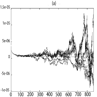
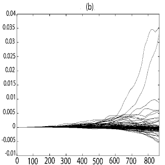
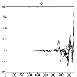
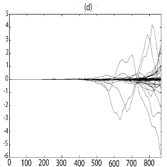
Figure 1: $\Delta D/D$ against t (simulation units) for $\alpha=0.0001,0.001,0.005,0.01$ (from top to bottom, following pannels (a) to (d)).

V Discussion

Our stochastic simulations suggest that the presence of random forces under the cosmic fluid description can lead to significant deviations from the non-stochastic solution for the growing mode at late times. In fact, for intensity levels of a Wiener process higher than $10^{-3}$, the stochastic contribution to the growth factor would be of the same order as the predictions of typical differences between ${\rm\Lambda}$CDM model and dark energy models [22]. Hence, this noise contribution would imply an additional difficulty to rule out models using large-scale structure data. In the present work, the introduction of stochasticity is completely ad hoc and our toy model based on the amplification of a Wiener process is quite arbitrary. However, our purpose is just to figure out if such contribution could be relevant to cosmology even for a simple implementation of the noise term. Actually, if noise should enter or not in the cosmic density evolution description is still a matter of debate, see e.g. [4]. Our results just raise the problem of distinguishing cosmological models using structure formation in the context of a cosmic fluid with underlying random forces. Of course, to pursue this effect more properly, theoretical efforts are necessary in order to understand the expected noise levels ab initio and the correct way to model and introduce them in the fluid description.

- (1) References
- (2)
- (3) Jeans, J.H., Phil. Trans. Roy. Soc, 199, 1 (1902)
- (4) Lifshitz, E.M., J. Phys. Acad. Sci. (USSR), 10, 116 (1946)
- (5) Longair, M. in Galaxy Formation, Springer, Berlin (1998)
- (6) Buchert, T., Dominguez, A. and Pérez-Mercader, J., Astronomy and Astrophysics, 349, 343 (1999)
- (7) Barbero, J.F., Dominguez, A., Goldman, T., and Pérez-Mercader, J., Europhys. Lett, 38, 637 (1997)
- (8) Dominguez, A., Hochberg, D., Martín-Garcia, J.M., Pérez-Mercader, J. and Schulmann, L., Astronomy and Astrophysics, 344, 27 (1999)
- (9) Kloeden, E. and Pearson, R.A., J. Austr. Soc., B20, 1 (1977)
- (10) Linder, E.V. and Jenkins, A., MNRAS, 346, 573 (2003)
- (11) Benabed, K. and Bernardeau, F., Phys. Rev. D, 64, 083501 (2001)
- (12) Peebles, P.J.E., in Large Scale Structure of the Universe, Princeton University Press, 1980.
- (13) Lifshitz, E.M. and Pitaevskii, L.P., in Statistical Physics, Part 2 (Course of Theoretical Physics, Vol. 9) Pergamon Press, Oxford (1980)
- (14) Sobczyk, K., in Stochastic Differential Equations, Kluwer Academic Publishers, Dordrecht (1991)
- (15) Knobloch, E., Vistas in Astronomy, 24, 39 (1980)
- (16) Kloeden, E. and Platen, E., in Numerical Solution of Stochastic Differential Equations, Springer, Berlin (1992)
- (17) Kloeden, E., Platen, E. and Schurz, H., in The Numerical Solution of Stochastic Differential Equations Through Computer Experiments, Springer, Berlin (1993)
- (18) Riess, A. et al., AJ, 116, 1009 (1998)
- (19) Perlmutter, S. et al., ApJ, 517, 565 (1999)
- (20) Tegmark, M. et al., Phys. Rev. D 69, 103501 (2004)
- (21) Eisenstein, D.J. et al., ApJ, 633, 560 (2005)
- (22) Turner, M. & Huterer, D., astro-ph/07062186
- (23) Frieman, J.A., Turner, M. and Huterer, D., astro-ph/0803.0982
- (24) Chongchitnan, S. and Efstathiou, G., Phys. Rev. D 76, 043508 (2007)
- (25) Weinberg, S. ApJ, 168, 175 (1971)