Structural Symmetry of Two-dimensional Metallic Arrays: Implications for Surface Plasmon Excitations

Abstract

In recent years, there has been intensive investigation of surface plasmon polaritons (SPPs) in the science and engineering fields. Understanding the physics of surface plasmon excitation is essential to the manipulation of SPPs, and most existing studies focus on ($-1,0$)-type SPP excitation. In this article, we report our recent investigation of the ($0,\pm 1$)-type SPP excitation of a gold two-dimensional nano-cavity array using finite-difference time-domain methodology. Our particular focus is on the symmetry properties of ($0,\pm 1$)-SPPs excited by different polarizations of light. It is found that polarization has strong implications for the field distribution of the corresponding SPPs. As a result, the control of polarization may provide important insights into the manipulation of SPPs.

I Introduction

Recent advances in nanotechnology have ignited the study of surface plasmon polaritons (SPPs), which have become a popular topic Garcíe de Abajo (2007); Barnes et al. (2003); Raether (1988) due to their wide range of potential applications in surface-enhanced Raman scattering (SERS) Kneipp et al. (2006), surface enhanced second harmonic generation, nano-photonics Lal et al. (2007), thermal-photovoltaic devices Wilde et al. (2006); Billaudeau et al. (2008); Greffet et al. (2002); Wan (2009), and data storage and imaging Schmidt et al. (2008)

However, finding a way to excite and control SPPs in an advantageous manner is still the main concern of scientists. The technology available to control SPPs with precision and flexibility remains underdeveloped, and different schemes have been proposed in this regard. For example, since the discovery of extraordinary transmission Ebbesen et al. (1998), major interest has centered on investigating cylindrical hole arrays in which subwavelength hollow cylinders are periodically formed on a flat metal film using lithographic methods Barnes et al. (2004); Popov et al. (2000). The work of Kelf et al. (2005), however, has demonstrated showed that the shape of an individual cavity in metallic grating plays a dominant role in controlling the excitation of SPPs. In addition, van der Molen et al. (2005) showed that there are shape and localized resonances in two-dimensional (2D) periodic subwavelength metallic cavity arrays. As a result, different shapes can lead to different resonances because the holes act like plasmonic cavities to confine the electric field and thereby give rise to strong localized resonances Garcíe de Abajo (2007); Moreno et al. (2006); Baida and Van Labeke (2003). Understanding the geometry effects of cavities can lead to a number of applications that require the precise spatial and frequency control of an enhanced electric field, such as SERS and thermal radiation. However, scientists have only a limited understanding of the surface shape resonances, and the correlation between SPP excitation and cavity geometry has not been widely investigated until recently (Kelf et al., 2005; Sepulveda et al., 2008; Sauvan et al., 2008; Chuang et al., 2008; Li et al., 2008; Iu et al., 2008; Li et al., 2009; Chen et al., 2008). In a recent work, we reported the fabrication of 2D nano-cavity arrays on a gold surface using interference lithography (IL) Li et al. (2008). In this article, we focus on a theoretical study of 2D nano-cavity arrays by using finite-difference time-domain (FDTD) simulation Taflove and Hagness (2005) methodology. Our particular focus is on the symmetric properties and polarization dependence of excited SPPs

II Simulation details

II.1 Basic simulation cell setup

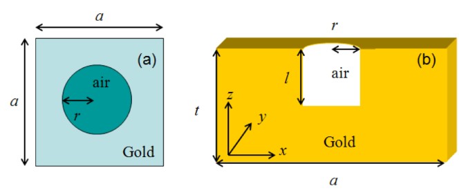
Figure 1: (Color online) (a) Unit cell and (b) top view of the cylindrical cavity.

We consider a model system that contains a gold slab drilled with a 2D array of cylindrical cavities. It is convenient to define the unit cell shown in Fig. 1 with suitable boundary conditions. Periodic boundary conditions (PBCs) are applied in both the $\pm x$- and $\pm y$-directions to produce a periodic structure. To account for non-periodicity in the $z$-direction, the perfectly matched layer (PML) Berenger (1994) boundary condition is adopted in the $\pm z$-directions. In addition, certain parameters are fixed throughout the study. For example, we only examine optical wavelengths that range from $400$ nm to $900$ nm. Moreover, the thickness of the gold layer is set at $1$ $\mu$m to ensure that the structure can be considered to be optically thick and such bulk photonic effects as Fabry-Pérot resonance and guiding mode resonance Fan and Joannopoulos (2002) are substantially reduced and negligible. Finally, the spatial and time resolution are $\Delta x=25$ nm and $\Delta t=\Delta x/c$, respectively, and the two lattice constants are fixed at $a=575$ nm.

II.2 Dielectric function of gold

Gold processes complex electron inter-band transitions at infrared frequencies. As a result, simple dielectric functions such as the Drude model, which considers only the electric response of conduction electrons, may not be adequate for modeling the dielectric response of gold. In this work, the multiple Drude-Lorentz model proposed by Vial et al. (2005) is adopted:

$$\tilde{\varepsilon}(\omega)=\varepsilon_{\infty}-\sum_{j}\frac{\triangle\varepsilon_{j}\omega_{j}^{2}}{\omega_{j}^{2}-\omega^{2}-i\omega\gamma_{j}}.$$ (1)

Here, index $j$ represents the contribution to the dielectric function made by the electrons of different bands; $\omega_{j}$ and $\gamma_{j}$ are the frequency and damping parameters; $\varepsilon_{\infty}$ is the high-frequency response, which is originated by the screening of the core electrons; and, finally, $\Delta\varepsilon_{j}=\epsilon_{\infty}-\varepsilon_{j}$, where $\varepsilon_{j}$ is the static dielectric response contributed by the different electron bands. Equation (1) is fitted against the measured dielectric function of gold (Palik, 1985), and the fitted parameters are tabulated in Table 1. Figure 2 shows both the measured and fitted dielectric functions. As can been seen, Eq. (1) agrees well with the measured $\varepsilon$ throughout our frequency range of interest.

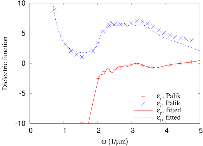
Figure 2: (Color online) The real ($\varepsilon_{\rm r}$) and imaginary ($\varepsilon_{\rm i}$) parts of the dielectric function fitted with the multiple Drude-Lorentz model.

$\varepsilon_{\infty}$	$\triangle\varepsilon_{i}$	$\omega_{i}$ $(1/\mu m)$	$\gamma_{i}$ $(1/\mu m)$
5.339	6.2634$\times 10^{41}$	0.0486	1$\times 10^{-20}$
	0.1906	2.1201	0.1772
	0.9835	4.4214	1.9662
	1.5974	3.353	1.1844
	0.6653	2.7116	0.578
	0.4508	2.3525	0.3012

Table 1: (Color online) Fitted parameters for Eq. 1.

II.3 Dispersion relation calculation

To calculate the dispersion relation, several Gaussian sources are placed within the simulation cell. These Gaussian sources have a frequency width that covers the entire optical frequency range. They are randomly located so that all of the resonant modes of the system can be excited. After turning off the sources, some fields are left in the system to allow their magnitudes to be recorded as a finite-length signal. This signal is then expressed as the sum of a finite number of sinusoids with exponentially decaying factors in a given bandwidth. The frequencies, decay constants, amplitudes, and phases of these sinusoids are determined from the coefficients of the sum.

Furthermore, line sources pointing in the $y$-direction are used to allow an investigation of the effects of different polarizations on the dispersion relations. These sources can be classified as $p$-polarized or $s$-polarized, depending on whether it is the magnetic field ($H_{y}$) or electric field ($E_{y}$) that pointis in the $y$-direction, respectively.

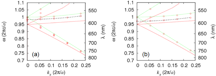
Figure 3: (Color online) Dispersion relations of an $r=75$ nm cylindrical cavity array under (a) $p$-polarized and (b) $s$-polarized lights. The green dotted lines are Wood’s anomalies [Eq. (2)], the red lines are the SPP dispersions of a gold slab [Eq. (3)], and the black dotted lines are the calculated ($0,\pm 1$) modes.

Some of the resonant modes shown in Fig. 3 correspond to Wood’s anomalies (Barnes et al., 2004). Wood’s anomalies occur when one diffracted order is parallel to the structure surface, which results in energy redistribution to the other diffracted orders. In other words, the incident light is scattered in parallel to the structure surface. This causes a sudden change in reflectance when the frequency ($\omega$) and in-plane wave vector ($k_{x}$) of the incident light satisfies

$$\omega=c|\vec{k}|=c|\vec{k}_{x}+n\vec{G}_{x}+m\vec{G}_{y}|,$$ (2)

where $\vec{k}$ is the incident wave-vector, $\vec{G}_{x}$ and $\vec{G}_{y}$ are the reciprocal lattice vectors, and $n$ and $m$ are integers. Additionally, we can trace the SPPs by plotting their dispersion relation driven by the following equation

$$\omega=c\sqrt{\frac{\varepsilon_{\rm Au}+\varepsilon_{\rm air}}{\varepsilon_{\rm Au}\varepsilon_{\rm air}}}|\vec{k}_{x}+n\vec{G}_{x}+m\vec{G}_{y}|.$$ (3)

It can be seen that Eq. (3) agrees well with the remaining excited modes of the $p$-excited resonances for $(n,m)$ = $(-1,0)$, $(1,0)$, and $(0,\pm 1)$, whereas only the $(0,\pm 1)$-type resonances are present for $s$-polarization. This is due to the fact that the array has $C_{4v}$ point group symmetry. The eigenstates with $\vec{k}$ parallel to the $\Gamma$-$X$ direction are irreducible representations of point group $C_{1h}$ (Sakoda, 2001), and each eigenstate is either symmetric ($A$ mode) or antisymmetric ($B$ mode) under a mirror transformation along the $x$-$z$ plane and can be excited only by incident waves that have the same symmetric property. These are, as is discussed in Appendix A, $p$- and $s$-polarized lights, respectively. Furthermore, it is proven that only a symmetric eigenstate is present for ($n,m$) = ($-1,0$) and ($1,0$), but that, on the contrary, both symmetric and antisymmetric eigenstates exist for ($n,m$) = ($0,\pm 1$). Therefore, the black dotted lines shown in Figs. 3(a) and (b) represent the eigenstates of the $A$ and $B$ symmetries, respectively.

III Results and discussion

III.1 Field pattern calculation

We are now in a position to present the field density distribution of the various excited SPP modes. Guided by the dispersion relations, we have located the wave-vectors and frequencies of these excited modes at $k_{x}=0.1725$, $\omega=0.9968$ for the $p$-excited resonance from Fig. 3(a) and $k_{x}=0.1725$, $\omega=0.9849$ for the $s$-excited resonance from Fig. 3(b), respectively, and have calculated their corresponding near field intensities. To calculate field intensity, a plane-wave Gaussian source is put above the array at $z=1$ $\mu$m to mimic an incident beam. The source has a narrow frequency width, such that it simulates a single-frequency incident plane wave. In addition, a spatially dependent amplitude function, exp($2\pi ik_{x}x$), is added to the source, where $k_{x}$ is the in-plane wave-vector, such that the angle of incidence is given by $\sin^{-1}(k_{x}c/\omega)$.

This simulation provides us with useful information on the way in which the incident light interacts with the array and the physical properties of the excited resonances. Time-domain simulations provide information about both the transient and steady states. We focus on the steady states by calculating the spectral field density of an excited mode at specified $k_{x}$, $\omega$ values:

$$|\vec{E}(\vec{r},\omega)|^{2}=\int(\vec{E}^{*}(\vec{r},t)\cdot\vec{E}(\vec{r},t))e^{i\omega t}dt.$$ (4)

Consider the time-average of energy density, as follow

$$\int(\vec{E}^{*}(\vec{r},t)\cdot\vec{E}(\vec{r},t))dt$$

$$= \int(\int\vec{E}^{*}(\vec{r},\omega)e^{-i\omega t}d\omega\cdot\int\vec{E}(\vec{r},\omega^{\prime})e^{i\omega^{\prime}t}d\omega^{\prime})dt$$

$$= \int\int(\vec{E}^{*}(\vec{r},\omega)\cdot\vec{E}(\vec{r},\omega^{\prime}))(\int e^{i(\omega^{\prime}-\omega)t}dt)d\omega d\omega^{\prime}$$

$$= \int\int(\vec{E}^{*}(\vec{r},\omega)\cdot\vec{E}(\vec{r},\omega^{\prime}))2\pi\delta(\omega^{\prime}-\omega)d\omega d\omega^{\prime}$$

$$= 2\pi\int(\vec{E}^{*}(\vec{r},\omega)\cdot\vec{E}(\vec{r},\omega))d\omega.$$

Spectral field density is a single $\omega$ component of $\vec{E}^{*}(\vec{r},\omega)\cdot\vec{E}(\vec{r},\omega)$. Theoretically, we need to sum up all of the $\omega$ components. However, as the Gaussian source used has only a narrow frequency width, $\Delta\omega$, the component of the specified central frequency, $\omega_{\rm cen}$ dominates the integral. By assuming the other $\omega_{\rm others}$ components are weak, that is,

$$|\vec{E}(\vec{r},\omega_{\rm cen})|^{2}>>|\vec{E}(\vec{r},\omega_{\rm others})|^{2},$$ (5)

we have

$$|\vec{E}(\vec{r},\omega_{\rm cen})|^{2}=\int\vec{E}^{*}(\vec{r},t)\cdot\vec{E}(\vec{r},t)dt.$$ (6)

In addition, $|\vec{E}(\vec{r},\omega_{\rm cen})|^{2}$ also provides information about the harmonic eigenstate with a specified $k_{x}$ and $\omega_{\rm cen}$.

III.2 Symmetry properties of the excited SPPs

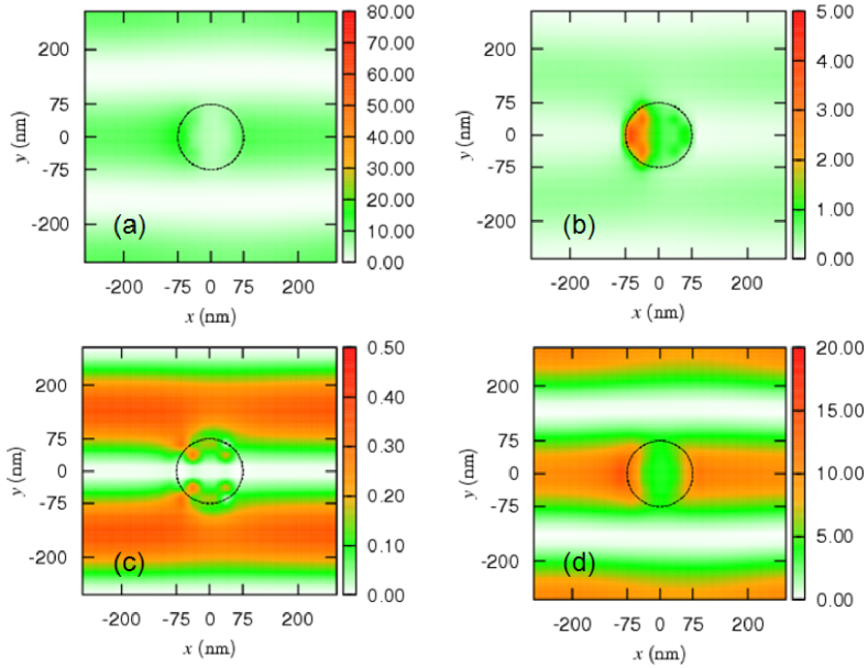
Figure 4: (Color online) Electric field density on $z=0$ of the ($0,\pm 1$) SPP mode of an $r=75$ nm cavity array excited by a $p$-polarized light: (a) $|E(\vec{r},\omega)|^{2}$, (b) $|E_{x}(\vec{r},\omega)|^{2}$, (c) $|E_{y}(\vec{r},\omega)|^{2}$, and (d) $|E_{z}(\vec{r},\omega)|^{2}$. The in-plane wavevector and frequency of the excited SPP are $0.1275$ and $0.9968$, respectively. The fields are not drawn to scale for better visibility. Note the symmetry along $y=0$ and $y=\pm a/2$.

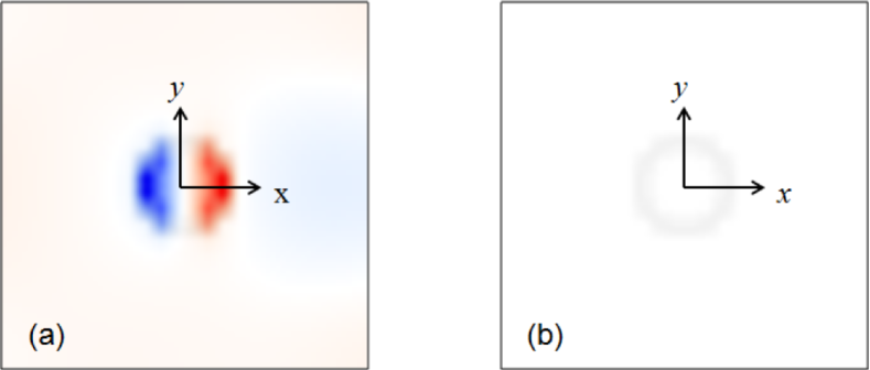
Figure 5: (Color online) Snapshots of the electric field distributions, $\vec{E}(\vec{r},t)$, for the $p$-excited SPP mode of Fig. 4, shown in (a) and (b), which are $E_{x}(\vec{r},t)$ and $E_{y}(\vec{r},t)$, respectively ($E_{y}$ is weak and can barely be observed). Note the symmetry along $y=0$. Blue and red represent positive and negative values, respectively.

In this section, we present the calculated field densities of the excited ($0,\pm 1$)-SPPs and discuss their symmetry properties. A general discussion of the symmetric properties of the eigenstates (Joannopoulos et al., 1995; Sakoda, 2001) is given in Appendix A. Electric field density ($|\vec{E}(\vec{r},\omega)|^{2}$) under $p$- and $s$-polarized excitations is shown in Figs. 4(a)–(d) and Figs. 6(a)–(d), respectively. The colors indicate field strength, which ranges from 0–80 arbitrary units (A.U.). The cavity is outlined with black dotted lines. As can been seen in Fig. 4(a), strong electric fields are distributed along the $x$-axis ($y=0$), with the strongest being concentrated near the rim of the cavity. This is in accordance with Eqs. (18)–(20), where $E^{2}_{x}$ [Fig. 4(b)] and $E^{2}_{z}$ [Fig. 4(d)] are symmetric along the $x$-$z$ plane, and $E^{2}_{y}$ [Fig. 4(c)] is anti-symmetric. Therefore, $E^{2}_{y}=0$ along $y=0$ and $y=\pm a/2$. In contrast, the field is asymmetric along the $x=0$ plane, which is due to the propagating nature of the excited SPP mode (Iu et al., 2008). When calculating the $|\vec{E}(\vec{r},\omega)|^{2}$, two kinds of electric fields are present in the system: one is the electric field of the resonant mode, labeled $\vec{E}_{\rm res}(\vec{r},\omega)$, and the other is the electric field of the incident light, labeled $\vec{E}_{\rm inc}(\vec{r},\omega)$. According to group theory, these two electric fields should have the same symmetric properties under $C_{1h}$ symmetric operations. The $p$-polarized light contains an electric field at the incident plane (the $x$-$z$ plane) whose time average is always symmetric along the $y=0$ plane, but asymmetric along the $x=0$ plane. As a result, the resultant field density, $|\vec{E}(\vec{r},\omega)|^{2}$, is asymmetric along the $x=0$ plane.

To further investigate the $p$-excited $(0,\pm 1)$ SPP, we show in Fig. 5 a snapshot of the field: $E_{x}(\vec{r},t)$ and $E_{y}(\vec{r},t)$ during the FDTD simulations. The symmetry conditions, $E_{x}(x,y,z)=E_{x}(x,-y,z)$ [Eq. (18)] and $E_{y}(x,y,z)=-E_{y}(x,-y,z)$ [Eq. (19)], can be observed clearly in the figures, although $E_{y}$ is too week and can barely be observed. It should be noted that the $x$-component of the electric field is very weak at $x=0$, and is mainly concentrated at ($x=\pm r$), which suggests that the local field should, at least to the first order, be dominated by point dipole-like distribution, (that is, $E_{x}\propto p_{x})$, where $p_{x}$ is the total dipole moment along the $x$-axis. This is in accordance with the hypothesis of Teperik et al. (2005), who treats each cavity as a resonator that consists of a simple capacitor, an inductor and resistance.

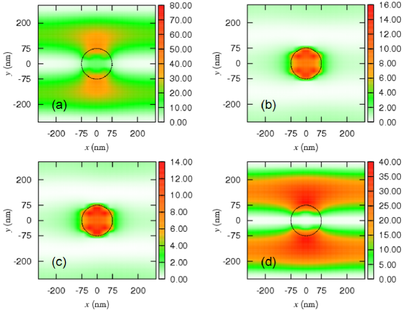
Figure 6: (Color online) Electric field density on $z=0$ of the $s$-excited ($0\pm 1$) SPP mode, $k_{x}=0.1275$ and $\omega=0.9849$. The symmetry along $x=0$ and $y=0$ indicates the localized nature of the resonance.

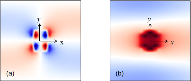
Figure 7: (Color online) Snapshots of the electric field distribution of the $s$-excited SPP mode in Fig. 6.

We next turn our attention to the $s$-excited ($0,\pm 1$) SPP modes, $|\vec{E}(\vec{r},\omega)|^{2}$, under $s$-polarized excitation, as shown in Figs. 6(a)–(d). According to Eqs. (18)–(20), $E_{x}$ and $E_{z}$ should be anti-symmetric and $E_{y}$ should be symmetric along $y=0$, which can be observed in Figs. 6(b)–(d). It should be noted that the field densities of $E^{2}_{x}$ and $E^{2}_{y}$ are very similar. However, as is revealed in Figs. 7(a)–(b), $E_{x}$ and $E_{y}$ are actually very different from each other. Moreover, it should also be noted that $E_{y}$ can be attributed to an effective dipole along the $y$-axis. In other words, $E_{y}\propto p_{y}$, which is similar to the case for $E_{x}$ in the $p$-excited ($0,\pm 1$) mode [Figs. 4(a) and 5(a)].

III.3 Conclusion

The present analysis relies only on the knowledge of $C_{4v}$-point group symmetry, which should be valid for any plasmonic structure that belongs to the same point group. Therefore, our argument can be applied to all $C_{4v}$-point group structures, such as square cavities, cross-shape grooves, circular crafters, pyramidal structures (Chuang et al., 2008; Chen et al., 2008), and bottle-shape cavities (Li et al., 2008; Iu et al., 2008). Additionally, SPP excitation along the $\Gamma$-M direction also has similar symmetric properties (Sakoda, 2001), and the corresponding eigenmodes can also be classified into even and odd modes, which are excited by $p$- and $s$-polarized light accordingly.

To sum up, we have performed FDTD analysis on a gold cylindrical cavity array and investigated the excited ($0,\pm 1$) mode based on the symmetry argument. Although very close in resonance frequencies, the even and odd modes display very different types of behavior in terms of field distribution, which has important implications for near-field applications such as SERS. It is hoped that this work will provide insight into the fields of plasmonics and nano-optics.

Appendix A Symmetric operations of eigenmodes

The eigenfunctions, $\vec{H}_{\vec{k}}(\vec{r},\omega)$, of a periodic plasmonic structure at eigenfrequency $\omega$ are Bloch functions that satisfy the master equation (Joannopoulos et al., 1995; Sakoda, 2001):

$$\hat{\Theta}\vec{H}_{\vec{k}}(\vec{r},\omega) = \nabla\times\left(\frac{1}{\varepsilon(\vec{r})}\nabla\times\right)\vec{H}_{\vec{k}}(\vec{r},\omega)$$ (7)

$$= \frac{\omega^{2}}{c^{2}}\vec{H}(\vec{r},\omega),$$

where $\vec{k}$ denotes wavevectors within the first Brillouin zone. Consider a mirror transformation operator, $\hat{M}_{xz}$, along the $x$-$z$ plane that is mapped from $\mathbb{R}^{3}$ to $\mathbb{R}^{3}$ by

$$\tilde{x} = \hat{M}_{xz}x=x,$$

$$\tilde{y} = \hat{M}_{xz}y=-y,$$

$$\tilde{z} = \hat{M}_{xz}z=z.$$

Under this transformation, the $y$-coordinate obtains a minus sign, and the $x$- and $z$-coordinates remain the same. The vector fields are transformed by operator $\hat{O}_{xz}$, defined as

$$\hat{O}_{xz}(f(\vec{r})\vec{F}(\vec{r}))=f(\hat{M}_{xz}\vec{r})\hat{M}_{xz}(\vec{F}(\hat{M}_{xz}\vec{r})),$$ (8)

and thus,

$$\hat{O}_{xz}f(\vec{r}) = f(x,-y,z),$$ (9)

$$\hat{O}_{xz}E_{x}(x,y,z) = E_{x}(x,-y,z),$$ (10)

$$\hat{O}_{xz}E_{y}(x,y,z) = -E_{y}(x,-y,z),$$ (11)

$$\hat{O}_{xz}E_{z}(x,y,z) = E_{z}(x,-y,z).$$ (12)

However, vectors defined by cross products are transformed differently. For example, for magnetic field $\vec{B}$,

$$\vec{F} = q\vec{v}\times\vec{B},$$

$$F_{x}\hat{x}+F_{y}\hat{y}+F_{z}\hat{z} = \left|\begin{array}[]{ccc}\hat{x}&\hat{y}&\hat{z}\\ v_{x}&v_{y}&v_{z}\\ B_{x}&B_{y}&B_{z}\\ \end{array}\right|$$

$$= (v_{y}B_{z}-v_{z}B_{y})\hat{x}$$

$$+ (v_{z}B_{x}-v_{x}B_{z})\hat{y}$$

$$+ (v_{x}B_{y}-v_{y}B_{x})\hat{z}.$$

To preserve the transformation properties of the force and velocity, the magnetic field is transformed as follows

$$\hat{O}_{xz}B_{x}(x,y,z) = -B_{x}(x,-y,z),$$ (14)

$$\hat{O}_{xz}B_{y}(x,y,z) = B_{y}(x,-y,z),$$ (15)

$$\hat{O}_{xz}B_{z}(x,y,z) = -B_{z}(x,-y,z).$$ (16)

Electric fields and magnetic fields are transformed in different ways under the mirror transformation.  

It is well known that $\hat{\Theta}$ commutes with $\hat{O}_{xz}$ for periodic structures:

$$\hat{\Theta}\hat{O}_{xz}=\hat{O}_{xz}\hat{\Theta}.$$

Also, if $\vec{k}=k\hat{x}$, then we have

$$\hat{O}_{xz}\vec{k}=\vec{k},$$

and

$$\hat{O}_{xz}\vec{H}_{\vec{k}}(x,y,z)=\pm\vec{H}_{\vec{k}}(x,y,z).$$ (17)

That is, the eigenmode is either symmetric ($+$) or antisymmetric ($-$) under mirror transformation along the $x$-$z$ plane. The substitution of Eqs. (10)–(12) and (14)–(16) into Eq. (17) gives

$$E_{\vec{k},x}(x,y,z) = \pm E_{\vec{k},x}(x,-y,z),$$ (18)

$$E_{\vec{k},y}(x,y,z) = \mp E_{\vec{k},y}(x,-y,z),$$ (19)

$$E_{\vec{k},z}(x,y,z) = \pm E_{\vec{k},z}(x,-y,z),$$ (20)

$$H_{\vec{k},x}(x,y,z) = \mp H_{\vec{k},x}(x,-y,z),$$ (21)

$$H_{\vec{k},y}(x,y,z) = \pm H_{\vec{k},y}(x,-y,z),$$ (22)

$$H_{\vec{k},z}(x,y,z) = \mp H_{\vec{k},z}(x,-y,z)$$ (23)

for eigenmodes that satisfy Eq. (17). In addition, for $p$-polarized lights, $\vec{E}=(E_{x},0,E_{z})$, $\vec{H}=(0,H_{y},0)$, and

$$E_{x}(x,y,z) = E_{x}(x,-y,z),$$

$$E_{z}(x,y,z) = E_{z}(x,-y,z),$$

$$H_{y}(x,y,z) = H_{y}(x,-y,z).$$ (24)

In contrast, $\vec{E}=(0,E_{y},0)$ and $\vec{H}=(H_{x},0,H_{z})$ for $s$-polarized lights; therefore

$$E_{y}(x,y,z) = E_{y}(x,-y,z),$$

$$H_{x}(x,y,z) = H_{x}(x,-y,z),$$

$$H_{z}(x,y,z) = H_{z}(x,-y,z).$$ (25)

A comparison of Eqs. (24) and (25) to Eqs. (18)–(23) suggests the $p$- and $s$-polarized lights are symmetric and antisymmetric to the $x$-$z$ plane mirror transformation, respectively. Therefore, the symmetric (+) modes can be excited only by $p$-polarized light that contains a symmetric electric field along the $x$-$z$ plane. Similarly, antisymmetric modes ($-$) can be excited only by $s$-polarized light.

References

- Garcíe de Abajo (2007) F. J. Garcíe de Abajo, Rev. Mod. Phys 79, 1267 (2007).
- Barnes et al. (2003) W. L. Barnes, A. Dereux, and T. W. Ebbesen, Nature 424, 824 (2003).
- Raether (1988) H. Raether, Surface Plasmons on Smooth and Rough Surfaces and on Gratings (Springer, Berlin, 1988).
- Kneipp et al. (2006) K. Kneipp, M. Moskovits, and H. Kneipp, eds., Surface-Enhanced Raman Scattering: Physics and Application (Springer, Berlin, 2006).
- Lal et al. (2007) S. Lal, S. Link, and N. J. Halas, Nat. Photon. 1, 641 (2007).
- Wilde et al. (2006) Y. D. Wilde, F. Formanek, R. Carminati, B. Gralak, P.-A. Lemoine, K. Joulain, J.-P. Mulet, Y. Chen, and J.-J. Greffet, Nature 444, 740 (2006).
- Billaudeau et al. (2008) C. Billaudeau, S. Collin, F. Pardo, N. Bardou, and J.-L. Pelouard, Appl. Phys. Lett. 92, 041111 (2008).
- Greffet et al. (2002) J.-J. Greffet, R. Carminati, K. Joulain, J.-P. Mulet, S. Mainguy, and Y. Chen, Nature 416, 61 (2002).
- Wan (2009) J. T. K. Wan, Opt. Commun. (2009), in press.
- Schmidt et al. (2008) M. A. Schmidt, L. N. Prill Sempere, H. K. Tyagi, C. G. Poulton, and P. S. J. Russell, Phys. Rev. B 77, 033417 (2008).
- Ebbesen et al. (1998) T. W. Ebbesen, H. J. Lezec, H. F. Ghaemi, T. Thio, and P. A. Wolff, Nature 391, 667 (1998).
- Barnes et al. (2004) W. L. Barnes, W. A. Murray, J. Dintinger, E. Devaux, and T. W. Ebbesen, Phys. Rev. Lett. 92, 107401 (2004).
- Popov et al. (2000) E. Popov, M. Neviere, S. Enoch, and R. Reinisch, Phys. Rev. B 62, 16100 (2000).
- Kelf et al. (2005) T. A. Kelf, Y. Sugawara, J. J. Baumberg, M. Abdelsalam, and P. Bartlett, Phys. Rev. Lett. 95, 116802 (2005).
- van der Molen et al. (2005) K. L. van der Molen, K. J. K. Koerkamp, S. Enoch, F. B. Segerink, N. F. van Hulst, and L. Kuipers, Phys. Rev. B 72, 045421 (2005).
- Moreno et al. (2006) E. Moreno, L. Martin-Moreno, and F. J. García-Vidal, J. Opt. A: Pure Appl. Opt. 8, S94 (2006).
- Baida and Van Labeke (2003) F. I. Baida and D. Van Labeke, Phys. Rev. B 67, 155314 (2003).
- Sepulveda et al. (2008) A. Sepulveda, Y. Alaverdyan, J. Alegret, M. Kall, and P. Johansson, Opt. Express 16, 5609 (2008).
- Sauvan et al. (2008) C. Sauvan, C. Billaudeau, S. Collin, N. Bardou, F. Pardo, and J.-L. Pelouard, Appl. Phys. Lett. 92, 011125 (2008).
- Chuang et al. (2008) S. Y. Chuang, H. L. C. andS. S. Kuo, Y. H. Lai, and C. C. Lee, Opt. Express 16, 2415 (2008).
- Li et al. (2008) J. Li, H. Iu, W. C. Luk, J. T. K. Wan, and H. C. Ong, Appl. Phys. Lett. 92, 213106 (2008).
- Iu et al. (2008) H. Iu, J. Li, H. C. Ong, and J. T. K. Wan, Opt. Express 16, 10294 (2008).
- Li et al. (2009) J. Li, H. Iu, J. T. K. Wan, and H. C. Ong, Appl. Phys. Lett. 94, 033101 (2009).
- Chen et al. (2008) H. L. Chen, S. Y. Chuang, W. H. Lee, S. S. Kuo, W. F. Su, S. L. Ku, , and Y. F. Chou, Opt. Express 17, 1636 (2008).
- Taflove and Hagness (2005) A. Taflove and S. C. Hagness, Computational Electrodynamics: The Finite-Difference Time-Domain Method (Artech House Publishers, Norwood, 2005).
- Berenger (1994) J.-P. Berenger, J. Comp. Phys. 114, 185 (1994).
- Fan and Joannopoulos (2002) S. Fan and J. D. Joannopoulos, Phys. Rev. B 65, 235112 (2002).
- Vial et al. (2005) A. Vial, A.-S. Grimault, D. Macias, D. Barchiesi, and M. Lamy de la Chapelle, Phys. Rev. B 71, 085416 (2005).
- Palik (1985) E. D. Palik, ed., Handbook of Optical Constants of Solids (Academic Press, New York, 1985).
- Sakoda (2001) K. Sakoda, Optical Properties of Photonic Crystals (Springer, Berlin, 2001).
- Joannopoulos et al. (1995) J. D. Joannopoulos, R. D. Meade, and J. N. Winn, Photonic Crystals: Molding the Flow of Light (Princeton Universiry Press, Princeton, N. J., 1995).
- Teperik et al. (2005) T. V. Teperik, V. V. Popov, and F. J. Garcíe de Abajo, Phys. Rev. B 71, 085408 (2005).