The Clustering of Mg II Absorption Systems at $z\sim 0.5$ and
detection of cold gas in massive halos

Abstract

We measure the large-scale clustering of Mg II $\lambda\lambda$ 2796,2803 absorbers with respect to a population of luminous red galaxies (LRGs) at $z\sim 0.5$. From the cross-correlation measurements between Mg II absorbers and LRGs, we calculate the mean bias of the dark matter halos in which the absorbers reside. We investigate possible systematic uncertainties in the clustering measurements due to the sample selection of LRGs and due to uncertainties in photometric redshifts. First, we compare the cross-correlation amplitudes determined using a flux-limited LRG sample and a volume-limited one. The comparison shows that the relative halo bias of Mg II absorbers using a flux-limited LRG sample can be overestimated by as much as $\approx$ 20%. Next, we assess the systematic uncertainty due to photometric redshift errors using a mock galaxy catalog with added redshift uncertainties comparable to the data. We show that the relative clustering amplitude measured without accounting for photometric redshift uncertainties is overestimated by $\approx 10$%. After accounting for these two main uncertainties, we find a 1-$\sigma$ anti-correlation between mean halo bias and absorber strength $W_{r}(2796)$ that translates into a 1-$\sigma$ anti-correlation between mean galaxy mass and $W_{r}(2796)$. The results indicate that a significant fraction of the Mg II absorber population of $W_{r}(2796)=1-1.5$ Å are found in group-size dark matter halos of $\log\,M_{h}<13.4$, whereas absorbers of $W_{r}(2796)>1.5$ Å are primarily seen in halos of $\log\,M_{h}<12.7$. A larger dataset would improve the precision of both the clustering measurements and the relationship between equivalent width and halo mass. Finally, the strong clustering of Mg II absorbers down to scales of $\sim 0.3\ h^{-1}$ Mpc indicates the presence of cool gas inside the virial radii of the dark matter halos hosting the LRGs.

1. Introduction

Characterizing the structure and evolution of the cold gas in dark matter halos is a key element in current models of galaxy formation (e.g., Kereš et al. 2005). The fraction of cold and hot gas within dark matter halos and the rate at which gas is being accreted are essential to our understanding of disc and star formation (e.g., Dekel et al. 2009). Extended gaseous envelopes around galaxies were first predicted several decades ago (Spitzer 1956). Observations of H I maps around local galaxies (e.g., Thilker et al. 2004; Doyle et al. 2005) and comparisons of galaxies and QSO absorption-line systems (e.g., Bergeron & Stasińska 1986; Lanzetta & Bowen 1990; Steidel et al. 1994; Chen et al. 2001; Chen & Tinker 2008) have indeed shown the presence of extended cool gas ($T\sim 10^{4}$ K) out to $50-100\ h^{-1}$ kpc radii. The physical mechanism that explains the origin of the extended cold halo gas is, however, unclear. Some of the most common scenarios are (i) outflows from starburst systems (e.g., Bond et al. 2001); (ii) stripping from the accretion of gas-rich satellites (Wang, 1993); (iii) cold gas bound to substructure within the host dark halo (e.g., Sternberg et al. 2002), and (iv) a two-phase medium composed of cold and hot gas (Mo & Miralda-Escude, 1996; Maller & Bullock, 2004).

A potential probe of the cold halo gas is the Mg II $\lambda\lambda$ 2796,2803 absorption features commonly seen in the spectra of background QSOs. These absorbers are thought to originate in photo-ionized gas of temperature $T\sim 10^{4}$ K and to trace high-column density ${\rm H\,I}$ clouds of neutral hydrogen column density $N(\mbox{${\rm H\,I}$})\approx 10^{18}-10^{22}$ ${\rm cm^{-2}}$ (Bergeron & Stasińska, 1986; Rao et al., 2006). This large associated ${\rm H\,I}$ column density indicates that Mg II absorbers arise in halo gas around individual galaxies (Doyle et al., 2005). This is also supported by the presence of luminous galaxies at projected distances $\rho=50-100\ h^{-1}$ kpc from known Mg II absorbers (Bergeron, 1986; Lanzetta & Bowen, 1990; Bergeron & Boissé, 1991; Lanzetta & Bowen, 1992; Steidel & Sargent, 1992; Steidel et al., 1994; Zibetti et al., 2007; Nestor et al., 2007; Kacprzak et al., 2008).

In addition to the classical gas accretion scenario for the origin of Mg II absorbers at larger galactic radii, there is a competing scenario that has gained substantial attention recently. In this new picture, strong Mg II absorbers of rest-frame absorption equivalent width $W_{r}(2796)>1$ Å originate in starburst driven outflows (e.g., Bond et al. 2001; Ménard & Chelouche 2008; Weiner et al. 2008). Under this scenario, the Mg II absorbing gas orginates in the cold outflowing material surrounding starburst galaxies. An interesting recent finding is a strong correlation between dust extinction $E(B-V)$ and $W_{r}(2796)$ by Ménard et al. (2008). While the observed $E(B-V)$ vs. $W_{r}(2796)$ is consistent with the expectation of the starburst scenario, this observation is also expected if the Mg II absorbing galaxies exhibit a metallicity gradient commonly seen in regular galaxies (e.g., Zaritsky et al. 1994; van Zee et al. 1998). Dense clumps in starburst driven outflows are expected to contribute to some fraction of the observed Mg II absorbers, but the significance of this fraction and how the fraction varies with $W_{r}(2796)$ are both uncertain.

As a first step toward a quantitative understanding of the physical origin of the Mg II absorber population, we are carrying out a cross-correlation analysis of Mg II absorbers with photometrically identified luminous red galaxies (LRGs) in the Sloan Digital Sky Survey (SDSS; York et al. 2000). The primary goals are (1) to determine the clustering amplitude of Mg II absorbers and (2) to examine how the clustering amplitude depends on absorber strength $W_{r}(2796)$. The clustering amplitude of Mg II absorbers is determined based on their cross-correlation signals with LRGs on projected co-moving distance scales of $r_{p}=1-30\ h^{-1}$ Mpc. Because the mean halo mass of the LRGs can be calculated from their clustering signal (e.g., Zheng et al. 2008; Blake et al. 2008; Wake et al. 2008; Padmanabhan et al. 2008) the cross-correlation amplitude of LRGs and Mg II absorbers provides a statistical estimate of the mean mass of the host dark matter halos. A similar study was published by Bouché et al. (2004, 2006), in which the authors attempted to constrain the mean halo mass of Mg II absorbers using a flux-limited ($i^{\prime}<21$ mag) sample of LRGs found in SDSS (see also Lundgren et al. 2009).

Our analysis differs from others in two important aspects. First, we measure the clustering amplitude of Mg II absorbers using a volume-limited (instead of flux-limited) LRG sample. A flux-limited selection criterion forms an inhomogeneous sample of LRGs, excluding progressively more intrinsically fainter LRGs (and hence lower-mass halos) toward higher redshifts. Such inhomogeneous samples of LRGs over a broad redshift range ($z=0.35-0.8$) include an inherent uncertainty in the estimated mean halo mass that is difficult to assess, but this systematic bias has not been addressed in previous studies. We have directly compared the clustering amplitudes between using a flux-limited and a volume-limited LRG sample. We will show in the following sections that the relative halo bias of Mg II absorbers may have been overestimated by as much as $\approx$ 20% in previous studies.

Second, the LRGs in SDSS have been identified using photometric redshifts ($z_{\rm phot}$) that have associated uncertainties relative to spectroscopic redshifts ($z_{\rm spec}$) of $\sigma_{0}=|z_{\rm phot}-z_{\rm spec}|/(1+z_{\rm spec})\approx 0.03$ at $i^{\prime}\approx 19$ (Collister et al. 2007; Oyaizu et al. 2008). At fainter magnitudes, $\sigma_{0}$ increases steeply to $\sigma_{0}\geq 0.1$ at $i^{\prime}>20.7$ (Collister et al. 2007). It is clear from these studies that the redshift uncertainties of the LRG sample vary from $\sigma_{z}=\sigma_{0}(1+z)=0.04$ for galaxies of $i^{\prime}<19$ at $z=0.35$ to $\sigma_{z}=0.18$ for galaxies of $i^{\prime}\approx 21$ at $z=0.8$. On the other hand, Mg II absorbers are identified in QSO spectra with a redshift precision better than $\sigma_{z}\approx 0.0004$, corresponding to roughly half of the width of a resolution element. The dependence of photometric redshift errors on galaxy brightness and redshift are expected to introduce additional systematic uncertainties in the estimate of the Mg II-LRG cross-correlation amplitude. To reduce the systematic bias due to photometric redshift errors, we first restrict our analysis to including only galaxies brighter than $i^{\prime}=20$. This allows us to maintain an LRG sample of higher redshift precisions. In addition, we assess the systematic uncertainty using a mock galaxy catalog with and without an added $\sigma_{0}\times(1+z)$ redshift perturbation. We will show in the following section that relative clustering amplitude of Mg II absorbers measured without accounting for photometric redshift uncertainties may have been overestimated by $\approx 10$%.

This paper is organized as follows. We first describe our data samples, Mg II and LRGs in Section 2. In Section 3.1, we describe the method used to calculate the two-point correlation function and associated errors. Cross-correalation results are presented in section 3.2, including a discussion of the effects of photometric redshift uncertainties in the calculation. In Section 4, we summarize the routines adopted for calculating the bias and mean halo mass of absorbers. Finally, we discuss the results of our analysis in Section 5. A more extensive halo occupation distribution analysis of the Mg II absorbers will be the subject of a forthcoming paper. We adopt a $\Lambda$CDM cosmology, $\Omega_{\rm M}=0.25$ and $\Omega_{\Lambda}=0.75$, with a dimensionless Hubble parameter $h=H_{0}/(100\ {\rm km}\ {\rm s}^{-1}\ {\rm Mpc}^{-1})$ throughout the paper. All masses are expressed in units of $h^{-1}~{}M_{\odot}$ unless otherwise stated.

2. Data

2.1. MgII Catalog

The MgII absorbers catalog is based on an extension of the SDSS DR3 sample (Prochter et al., 2006) to include DR5 QSO spectra (J.X. Prochaska, private communication). This sample of Mg II absorbers has a 95% completeness for absorbers of $W_{r}(2796)>1$ Å. The catalog contains 11,254 Mg II absorbers detected at $z_{\rm Mg\,II}=0.37-2.3$ along 9,774 QSO sightlines. From this sample, we selected absorbers with a separation of at least 10,000 km/s from the QSO redshift to avoid contamination by associated absorbers of the QSOs. We excluded absorbers that fall outside of our survey mask (see Section 3.1.1) and we limited ourselves to Mg II doublets in the redshift range of interest, $z=0.40-0.70$, defined by the LRG sample. Note that none of the absorbers listed in the Prochter et al. catalog are found in the Ly$\alpha$ forest of their respective quasar. The procedure described above yielded 1,158 absorbers of $W_{r}(2796)>1$ Å. This contitutes our primary Mg II catalog. The short dashed histogram in Figure 1 shows the redshift distribution of our primary Mg II sample.

2.2. LRG Catalog

LRGs are tracers of the large-scale structures in the universe. Their clustering properties are well-known, and they reside in massive halos of $M_{h}>10^{13}\mbox{$h^{-1}\,{\rm M}_{\odot}$}$ (e.g., Blake et al. 2008; Zheng et al. 2008; Wake et al. 2008; Padmanabhan et al. 2008). Because they are luminous and have strong 4,000-Å break, their photometric redshift can be more reliably estimated than blue star-forming galaxies.

We used the MegaZ-LRG catalog (hereafter MegaZ) (Collister et al., 2007) as our initial LRG sample. MegaZ is a photometric redshift catalog of approximately $10^{6}$ LRGs found in the SDSS DR4 imaging footprint. The catalog covers more than 5,000 $\rm{deg}^{2}$ in the redshift range 0.4 $<$ $z$ $<$ 0.7. The LRGs are selected following a series of cuts in a multidimensional color diagram (e.g., Scranton et al. 2003; Eisenstein et al. 2005; Collister et al. 2007). The photometric redshifts of LRGs are determined using artificial neural networks (ANNz) and the 2SLAQ training set of 13,000 available LRGs spectroscopic redshifts (Cannon et al., 2006).

We applied a set of additional color selection criteria suggested by Blake et al. (2007). These modified criteria yielded less contamination by blue galaxies and were used in clustering and halo occupation analyses (Blake et al., 2008). We further limited ourselves to galaxies with $i^{\prime}<20$ for a higher photometric redshift precision. We defined three LRG samples for our analysis. The first was a flux-limited sample of $i^{\prime}<20$ LRGs at $z=0.4-0.7$. This primary sample covers the entire redshift range offered by the initial LRG sample. The second was a volume-limited sample of $M_{i^{\prime}}-5\,\log\,h<-22$ at $z=0.45-0.60$. The redshift range was selected to provide the largest number of LRGs available under a uniform minimum rest-frame absolute magnitude selection criterion. Extending to lower or higher redshifts would result in a significant reduction in the sample size. The third was a flux-limited sample of $i^{\prime}<20$ at $z=0.45-0.60$ to be directly compared with the volume-limited subsample from the same redshift range.

Our sample definition was motivated by the knowledge that a flux-limited sample contains galaxies that are progressively fainter at lower redshifts, whereas a volume-limited criterion identifies a uniform sample of galaxies that occupy the same luminosity interval at different redshifts. In addition, the cross- and auto-correlation calculations are evaluated at different redshift in a flux-limited sample. The redshift number density of LRGs peaks at $z\sim 0.45$, while the Mg II redshift distribution is flat. This implies that the mean redshifts of the cross-correlation and auto-correlation calculations are different, introducing additional uncertainties in the estimated mean halo bias. This problem is alleviated in a volume-limited sample because the cross- and auto-correlation terms have similar redshift evolution (see Figure 1). Comparing the correlation functions determined using different subsamples allowed us to evaluate possible systematic uncertainties due to sample selections.

The limiting absolute magnitude of the volume-limited sample was determined by calculating the absolute magnitude of our faintest galaxies ($i^{\prime}=20.0$) at the limiting redshift $z=0.60$

$$20.0-{M}_{i}={\rm DM}(z)+k(z)\;,$$ (1)

where ${\rm DM}(z)$ is the distance modulus and $k(z)$ represents the $k$-correction. At $z=0.60$, the limiting magnitude is $M_{i}-5\log h=-22$ and we found roughly 197 K galaxies more luminous than this limit. A quantitative description of the three LRG samples including the number of objects and redshift range can be found in Table 1. Figure 1 shows the redshift distributions of the three LRG samples and the top panel of Figure 2 shows the magnitude distributions of our flux-limited LRG sample and of the initial LRG sample.

It is notoriously difficult to determine the photometric redshift of faint galaxies. The bottom panel of Figure 2 shows a subsample of the photometric redshift errors taken for 1,000 overlapping galaxies between MegaZ and the SDSS photometric redshift table. The photoz’s errors shown in this figure are taken in the ”photozcc2” table found on the SDSS skyserver archive (Oyaizu et al., 2008). The photometric redshift errors obtained by the MegaZ team are consistent with the ones in Oyaizu et al. (2008) to within measurement uncertainties. However, it is clear from Figure 2 that for $i^{\prime}>20$, the uncertainties in the photoz’s increase rapidly. For this reason, we decided to restrict ourselves to LRG candidates with $i^{\prime}<20$. This procedure yielded a total of 962,216 MegaZ objects satisfying our additional selection criteria. This constitutes our primary LRG catalog.

Figure 1.— Redshift distributions of the initial MegaZ LRG sample and of the three LRG samples used in our correlation studies. The initial MegaZ catalog is shown in the dotted line. The solid line shows the flux-limited sample ($z=0.40-0.70$) and the dashed line shows the volume-limited sample ($z=0.45-0.6$). The redshift distribution of Mg II absorbers in our primary sample is overplotted in short-dashed line for comparison.

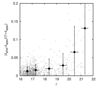
Figure 2.— Top panel: Magnitude distribution of the LRGs satisfying our selection criteria ($\approx 9.6\times 10^{5}$ LRGs). The line shows the $i^{\prime}$ magnitude distribution. Only galaxies with $i^{\prime}<20$ are included in our LRG sample. Bottom panel: Photometric redshift error versus $i^{\prime}$ magnitude for a subsample of 1,000 galaxies in SDSS taken from Oyaizu et al. (2008). The photometric errors are listed in the SDSS Table ”photozerr2” under ”CC2”. Black diamond points with error bars represent the mean and dispersion calculated in bins of $\Delta i^{\prime}=1$ mag.

3. Mg II absorbers-LRG cross-correlation

3.1. Method

We used the Landy & Szalay (1993) (LS93) minimum variance estimator to calculate the projected two-point correlation statistics between Mg II absorbers and LRGs. Using the LS93 estimator, the real-space correlation function can be calculated following

$$\xi(r_{p},\pi)=\frac{D_{\rm a}D_{\rm g}-D_{\rm a}R_{\rm g}-D_{\rm g}R_{\rm a}+R_{\rm a}R_{\rm g}}{R_{\rm a}R_{\rm g}}$$ (2)

where $R$ and $D$ are random points and data, the subscripts $a$ and $g$ refer to absorbers and galaxies, $r_{p}$ is the projected comoving separation between two objects on the sky and $\pi$ is their distance parallel to the line of sight. Note that the above two-point estimator has been successfully used in previous correlation study based on QSO absorbers and galaxy data collected from a smaller area survey (Adelberger et al., 2003). In practice, we calculated the projected two-point correlation statistics by summing all pairs along the sightline

$$w_{p}(r_{p})=\int_{l}\xi(r_{p},\pi)d\pi$$ (3)

and inside of redshift limits $l$ of our three LRG samples.

Another commonly used estimator, $1+\xi(r_{p},\pi)=\frac{D_{\rm a}D_{\rm g}}{D_{\rm a}R_{\rm g}}$ has also been used in the initial stages of this work for comparison and validation purposes. Even though this estimator is easier (no random absorbers) and faster (two terms to compute instead of four), the variance of $w_{p}$ is larger for this estimator than for LS93. For this reason, we employed the LS93 estimator for all $w_{p}$ calculations.

We divided the pairs into eight $r_{p}$ bins covering the range $0.2-35~{}h^{-1}$ Mpc. The bins were equally separated in logarithm space. The bin size and the $r_{p}$ value of the inner most bin were determined in such a way that at least 10 $DD$ pairs were found in that bin. The upper limit of $35~{}h^{-1}$ Mpc was chosen to be a few times smaller than the size of the jackknife cells (see section 3.1.3).

3.1.1 Survey mask

For the calculation of the two-point statistics (following equation 2) both data and randoms were distributed over the exact same survey mask. Different masks for LRGs and MgII would alter the shape and amplitude of the correlation signal in an undesirable fashion, especially at large separations. To make sure the sky coverage was the same for Mg II, LRGs and their randoms, we used the lowest common denominator for all : the DR4 spectroscopic sky survey mask. Indeed, Mg II absorbers were taken from the SDSS DR5 spectroscopic sample which includes the QSO sightlines inside the DR4 spectroscopic sky. The LRGs were found in the DR4 imaging sky which encompasses the DR4 spectroscopic sky. The main disadvantage of using this mask was that the number of rejected objects falling outside of the mask was large, $\approx 40\%$.

To be able to determine which Mg II absorbers and LRGs fell inside this DR4 spectroscopic mask, we used the mask catalog provided by the NYU Value-Added Galaxy Catalog team Blanton et al. (2005). The mask corresponds to the angular selection function describing the completeness of the SDSS spectroscopic across the sky. It is defined by spherical polygons. The completeness quantifies the fraction, inside each polygon, of galaxies with spectrocopic redshift. We used the angular selection function of the spectroscopic SDSS DR4 sky ($\rm{sdssdr4safe0res6d}$).

3.1.2 Generating random Mg II absorbers and LRGs

The right ascension and declination of the LRGs were randomly selected over the DR4 spectroscopic sky using the function ransack available in the Mangle software package (Hamilton & Tegmark, 2004; Swanson et al., 2008). The redshifts of the random galaxies were determined by sampling the redshift distribution of the LRG dataset. Determining the sky positions and redshifts of the random absorbers was not a straightforward process. The angular selection function of quasars follows the DR4 spectroscopic mask, but the mask defining the positions where absorbers can be found is limited to the actual coordinates of the QSOs themselves. Thus, the random absorbers must be distributed randomly among fixed QSO sightlines for which SDSS spectra are available. Assigning random Mg II this way eliminates any undesired bias due to the intrinsic clustering of QSO sightlines. We identified these sightlines from the Schneider et al. (2007) SDSS DR5 QSO catalog by selecting all QSOs falling inside our DR4 spectroscopic mask with redshifts large enough to allow for the detection of Mg II absorbers inside the redshift range of interest for our calculations ($z=0.40-0.70$). We found a total of $\approx 5.5~{}\times~{}10^{4}$ sightlines. The (ra,dec) positions of the random absorbers were determined by randomly selecting the coordinates of these sightlines. Redshifts were selected randomly from a top hat probability distribution function over $z=0.4-0.7$.

The number of random LRGs, $R_{g}$, and the number of random Mg II absorbers, $R_{a}$, were determined after running convergence tests with increasing number of randoms. We varied the number of each random set (Mg II and LRGs) independently until the measured $w_{p}$ approached asymptotic values. The numbers of randoms used in our $w_{p}$ calculation were $R_{a}=10^{5}$ and $R_{g}=4\times 10^{6}$ for Mg II and LRGs, respectively. It is important to note that increasing the number of random Mg II absorbers to a very large number in comparison with the number of available QSO sightlines ($\sim$ 55K) would not lead to a rapid convergence because we would simply be overcounting the same $D_{\rm g}R_{\rm a}$ pairs and no additional information would be gained.

3.1.3 Relative contribution of cosmic variance and photometric uncertainty to $w_{p}$ errors

We looked at two independent sources contributing to the error bars on $w_{p}$ : cosmic variance and photometric redshift errors. Photometric redshift errors are expected to affect the measurements of $w_{p}$’s in two different ways. First, redshift uncertainties are expected to increase the noise in the $w_{p}$ measurements due to uncertainties in the object positions. Second, redshift uncertainties are expected to systematically alter the $w_{p}$ measurements to lower values due to an inherent sample selection bias. A galaxy sample selected based on imprecise photometric redshifts contain galaxies from a broader redshift range than one selected based on precise spectroscopic redshifts, and consequently reducing the observed correlation signal by including additional uncorrelated pairs. In this section, we address random errors in the $w_{p}$ measurements due to cosmic variance and object distance uncertainties. We defer the discussion on the systematic errors of $w_{p}$ due to the sample selection bias to § 3.2.2.

We estimated the cosmic variance using the jackknife resampling technique. The sky was separated into $N=192$ (see section 3.2.1 for a justification of this number) cells of roughly equal survey area. The cosmic variance for each point $r_{p,i}$ corresponds to the $i$th-diagonal element of the covariance matrix was calculated using a jackknife resampling technique :

$${\rm COV}(w_{i},w_{j})=\frac{N-1}{N}\sum_{k=1}^{N}(w_{i}^{k}-\overline{w_{i}})(w_{j}^{k}-\overline{w_{j}})$$ (4)

and $k$ represents the iteration in which box $k$ was removed. The mean $\overline{w_{i}}$ was calculated for bin $i$ over all $w_{p}^{k}$’s.

The impact of the large uncertainties due to photometric redshifts on the size of the $w_{p}$ errors is not taken into account by the jackknife resampling technique alone. Previous works (e.g., Bouché et al. 2006; Blake et al. 2008) have focused primarily on cosmic variance in the calculation of the errors bars, but have not addressed additional random noise due to photometric redshift errors which are quite large ($\sigma_{z}\approx 0.05$ for $i^{\prime}<20$) compared to the redshift ($z=0.5$).

To account for the independent contribution of photoz’s uncertainties on the final $w_{p}$ error bars, we generated 100 independent realizations of the MegaZ catalog. For each one of them, we resampled the redshift of each individual galaxy according to a normal distribution $N(z_{\rm phot},\sigma_{z})$, where $z_{\rm phot}$ is the photometric redshift and $\sigma_{z}$ is the photometric redshift error of each galaxy. In this case, we followed the error function $\sigma_{z}=0.03(1+z)$ found in Collister et al. (2007) to assign photometric redshift errors to galaxies. A new mock LRG sample was then established according to the criteria discussed in § 2.2. We calculated $w_{p}$ for each one of these realizations and assigned the error contribution from redshift uncertainties to the final error budget of $w_{p}$ by calculating the dispersion among these 100 independent realizations.

We found that the size of the $w_{p}$ error bars was dominated by cosmic variance. The contribution of photometric redshift errors to the $w_{p}$ error budget was small, at most 20% for the smallest separation bin. It is negligible ($\sim 1\%$) at large separations where we calculated the relative clustering strength and absolute bias. For this reason, we decided to adopt the cosmic variance $\sigma_{i}$ as the error on $w_{p}$ and neglect the contribution of the photometric redshifts.

3.2. Results

This section addresses the cross- and auto-correlation results for the three LRG samples and the effect of photometric redshifts on the clustering amplitude. For each one of our three LRG samples, we considered three subsamples of Mg II absorbers: weak $W_{r}(2796)=1-1.5$ Å, strong $W_{r}(2796)=1.5-5$ Å, and all absorbers. A description of each correlation calculation can be found in Table 1. We also include the number of $DD$ pairs (equation 2) in the first bin and the number of data found in each subsample in columns (6), (7), and (8).

Table 1Summary of the cross- and auto-correlation calculations

			$W_{\rm{r,min}}(2796)^{a}$	$W_{\rm{r,max}}(2796)$	Number	Number	Number
Sample	$z_{\rm min}$	$z_{\rm max}$	(Å)	Å	DD pairs(1stbin)b	LRGs	Mg II
(1)	(2)	(3)	(4)	(5)	(6)	(7)	(8)
Volume-limited sample
V-weak(VW)	0.45	0.60	1.0	1.5	21	197,968	279
V-strong(VS)	0.45	0.60	1.5	5.0	13	197,968	257
V-all(VA)	0.45	0.60	1.0	5.0	34	197,968	536
Flux-limited samples
F1-weak(F1W)	0.45	0.60	1.0	1.5	47	517,549	279
F1-strong(F1s)	0.45	0.60	1.5	5.0	35	517,549	257
F1-all(F1A)	0.45	0.60	1.0	5.0	82	517,549	536
F2-weak(F2W)	0.40	0.70	1.0	1.5	88	618,086	541
F2-strong(F2S)	0.40	0.70	1.5	5.0	68	618,086	617
F2-all(F2A)	0.40	0.70	1.0	5.0	156	618,086	1158
LRGs auto-correlation
V-LRGs(VG)	0.45	0.60	-	-	6,977	197,968	-
F1-LRGs(F1G)	0.45	0.60	-	-	43,093	517,549	-
F2-LRGs(F2G)	0.40	0.70	-	-	55,062	618,086	-

3.2.1 Cross- and auto-correlation results

Figure 3 shows the cross- and auto-clustering results for the flux- and volume-limited samples of LRGs. For each one of these samples, the results are shown for the three Mg II subsamples in gray. We overplot the LRGs auto-correlation results in black. A clear feature of Figure 3 is that, for the three LRG samples considered, the clustering amplitude of weak absorbers is systematically higher than for strong ones. It is also interesting to note that after accounting for systematic bias due to redshift uncertainties (see § 3.2.2), weak Mg II absorbers appear to be unbiased (sharing the same clustering amplitude) with respect to LRGs in both flux-limited and volume-limited samples.

For each auto- and cross-correlation calculations, we estimated the correlated uncertainties between different $r_{p}$’s using the covariance matrix (see equation 4) and the normalized correlation matrix

$$\rho(w_{i},w_{j})=\frac{{\rm COV}(w_{i},w_{j})}{\sqrt{{\rm COV}(w_{i},w_{i}){\rm COV}(w_{j},w_{j})}}\;.$$ (5)

We performed a convergence test on the number of jackknife boxes. We made sure that the off-diagonal elements of the correlation matrix varied by less than 10% after doubling the number of boxes. We plot in Figure 4 the normalized correlation matrix $\rho(w_{i},w_{j})$ for all calculations, including the LRGs auto-correlation shown in the fourth column. Adjacent bins are strongly correlated for the auto-correlation functions of LRGs and, in all cases of the LRG–Mg II cross-correlation measurements, bins with large $r_{p}$ are more correlated.

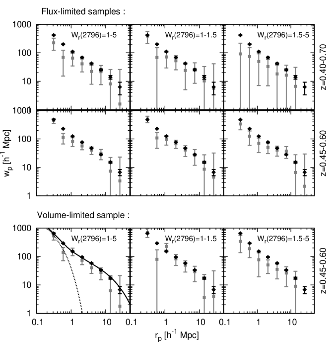
Figure 3.— Cross- and auto-correlation results for the flux and volume-limited samples of LRGs. From top to bottom, flux-limited sample $z=0.40-0.70$, flux-limited $z=0.40-0.60$, and volume-limited $z=0.40-0.60$. From left to right, all absorbers, weak absorbers and strong absorbers. The rest-frame equivalent-width coverage is listed at the top of each column. In all panels, the gray points represent the cross-correlation results (Mg II and LRGs) and the black points are for the LRGs auto-correlation. In the bottom left panel, we show the halo occupation distribution analysis done on the volume-limited sample of LRGs. The solid line shows the full HOD model and the dotted line the one-halo contribution (see section 4.2). Note that both cross- and auto-correlation results were corrected for photometric redshifts (see section 3.2.2). Error bars represent the 1-$\sigma$ jackknife errors calculated on $N=192$ sky boxes of equal area. Note that the last cross-correlation points in two of the strong Mg II absorber sample are negative and not displayed in these panels. The weak absorbers are essentially unbiased with respect to the LRGs and their clustering is strong, even down to 0.3 $h^{-1}$ Mpc.

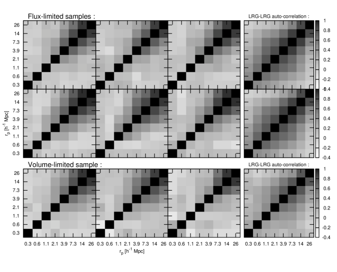
Figure 4.— Gray-scale plot of the correlation matrix (see equation 5) showing the degree of covariance between different separation bins. The different matrices shown correspond to the same calculations of Figure 3 for $W_{r}(2796)=1-5$ Å (left), $W_{r}(2795)=1-1.5$ Å (middle-left), and $W_{r}(2796)=1.5-5$ Å (middle-right), respectively. The fourth column shows the LRGs auto-correlation results.

3.2.2 Effect of photometric redshifts on the amplitude of clustering

An important effect of photometric redshift errors is the sample selection uncertainty. Photometric redshift uncertainties not only affect the precision of $w_{p}$, but also lower its accuracy that one would normally get from using spectroscopic redshifts (e.g., Brown et al. 2008). This needs to be accounted for in the bias calculation. One can think of photometric redshift errors as adding uncorrelated galaxies in the calculation, and the overall effect is an unwanted widening of the galaxy redshift distribution. This effect results in a systematic error in the clustering signal and the amplitude of $w_{p}$ is comparatively smaller than expected in calculations using only spectroscopic redshifts.

To estimate the attenuation of the clustering signal due to photometric errors, we performed several tests on mock LRG galaxy distributions. Our mock catalog is produced by populating the halos in an N-body simulation with a halo occupation function determined from the spectroscopic LRG sample in Zheng et al. (2008) (specifically, the “faint” sample). The simulation is large, 1 Gpc/h on a side, and represents our fiducial cosmology at $z\sim 0.5$ (see Tinker et al. 2008 for more details on this simulation). Since the box size is not big enough to cover the redshift range of our study, we mirror-imaged three identical copies of the box along the redshift direction. The mock LRG catalog has precise positions and therefore mimic a spectroscopic sample.

Three tests were performed. First, we auto-correlated the mock LRG sample without applying any modifications to their redshifts. This first case mimics the results one would get by auto-correlating a sample of LRGs with spectroscopic redshifts (the $w_{hh}$ case in Figure 6). Second, we cross-correlated the mock LRG sample with one that involved perturbed redshifts. The perturbed redshifts were generated by sampling a normal distribution centered on the input redshift in the mock catalog within $\sigma_{z}=0.03(1+z)$. That is the $w_{hh^{\prime}}$ term in Figure 5, which is in analogous to our cross-correlation measurements betwen absorbers with spectroscopic redshifts and galaxies with photometric redshifts. Third, we auto-correlated the mock LRG sample with perturbed redshifts ($w_{h^{\prime}h^{\prime}}$ in Figure 6). This mimics our LRG auto-correlation function.

We then computed the $w_{p}$ ratios between the different calculations and plotted the results in Figure 5. The three sets of symbols correspond to ratios of $w_{p}$ calculated over the same series of $r_{p}$ bins as in the correlation calculations shown in Figure 3. We show, by thick black lines, the best-fit amplitude of the three ratios in two different regimes : small and large separations. Best-fit values are listed in Table 2 with their corresponding uncertainties ($\Delta\chi^{2}<1$). Error bars on the ratios themselves correspond to the dispersion obtained among 100 realizations of a mock catalog with perturbed redshifts. The best-fit amplitude (of the light points) at large separation enters in the calculation of the relative bias (see section 5.1).

The dark datapoints in Figure 5 show that the cross-correlation function between Mg II absorbers and photometric redshift identified LRGs is underestimated by roughly 20% due to redshift errors. The gray points show that the auto-correlation function of these LRGs is underestimated by roughly 30%. Finally, the light-gray points show that the mean bias calculated based on the ratio of absorber-LRG cross-correlation and LRG auto-correlation functions is overestimated by roughly 10%.

Our estimated reduction in clustering strength of 10% is smaller than the value quoted in Bouché et al. (2004). These authors found that, in the case of a gaussian redshift distribution for galaxies, the amplitude of the MgII-LRG cross-correlation is overestimated by 25 $\pm$ 10%. They used numerical integration and mock galaxy catalog with phometric redshift uncertainties $\Delta_{z}=0.1$ corresponding to size of their redshift interval of interest. The discrepancy could be partly attributed to the larger photometric redshift uncertainties used by these authors.

Table 2Estimated reduction factor of the cross-correlation amplitude due to photometric redshift sampling errors

Measurement	$r_{p}<1~{}h^{-1}$ Mpc	$\chi^{2}$/D.O.F	$r_{p}>1~{}h^{-1}$ Mpc	$\chi^{2}$/D.O.F
$w_{\rm Mg\,II-LRG}$	0.77 $\pm 0.03$	1.35	0.79 $\pm 0.02$	0.26
$w_{\rm LRG-LRG}$	0.66 $\pm 0.04$	0.97	0.71 $\pm 0.04$	0.12

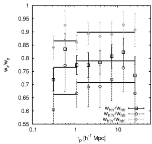
Figure 5.— Ratios of cross-correlation signals obtained from the simulation boxes to address the impact of photometric redshift uncertainties on the amplitude of $w_{p}$. Solid black : ratios of $w_{p}$’s where one of the two datasets has redshift position perturbed (within its error bars) ($w_{hh^{\prime}}$) over $w_{p}$’s obtained where both datasets have spectroscopic redshift ($w_{hh}$); dashed gray : ratios where both datasets have perturbed redshifts ($w_{h^{\prime}h^{\prime}}$) over two datasets with unperturbed redshifts ($w_{hh}$); Dotted light gray : $w_{p}$ for perturbed-perturbed datasets ($w_{h^{\prime}h^{\prime}}$) over perturbed-unperturbed ($w_{hh^{\prime}}$). The last set of points gives us an estimate of the systematic bias in the observed clustering amplitude of Mg II absorbers using photometric redshift identified LRGs. Error bars show dispersion among 100 realizations of the perturbed datasets ($h^{\prime}$). The thick solid lines represent best-fit amplitude obtained for the one ($r_{p}\leq 1.1h^{-1}$ Mpc) and two-halo ($r_{p}>1.1h^{-1}$ Mpc) terms. Best-fit values are listed in table 2. The best-fit amplitude obtained for the light gray points is used to correct for the addtional systematic error introduced by using photoz’s in the calculation of the correlation functions.

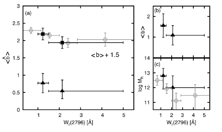
Figure 6.— Panel (a) shows the relative bias of Mg II for two of the three LRG samples. Solid lines with triangles are for the volume-limited sample, solid lines with squares for the flux-limited $z=0.40-0.70$, and open circles are taken from Bouché et al. (2006) for direct comparison with the flux-limited sample. For each LRG sample, the points are derived from the direct ratio of the points for $r_{p}>1~{}h^{-1}$ Mpc. The power-law technique yielded very similar results. We shifted the results for the flux-limited samples by $\langle\hat{b}\rangle+1.5$ for more clarity. Panel (b) : absolute bias for the volume-limited sample. Panel (c) bias-inverted halo mass derived from the absolute bias. The bias-weighted halo mass results of Bouché et al. (2006) are shown in open circles. Error bars along the x-axis represent the binning used.

Table 3Best-fit power-law $f(x)=ax^{b}$ results for the cross and auto-correlations.

1.5 Sample $a$ $b^{\rm i}$ $\chi^{2}$ $\chi^{2}/{\rm D.O.F}^{\rm ii}$ VW 0.337 $\pm 0.11$ -0.835 1.2 0.3 VS 0.206 $\pm 0.09$ -0.835 0.394 0.13 VA 0.275 $\pm 0.075$ -0.835 1.06 0.27 F1W 0.245 $\pm 0.080$ -0.783 0.54 0.14 F1S 0.194 $\pm 0.070$ -0.783 4.60 1.15 F1A 0.206 $\pm 0.056$ -0.783 3.78 0.76 F2W 0.160 $\pm 0.046$ -0.781 3.47 0.87 F2S 0.114 $\pm 0.047$ -0.781 0.776 0.258 F2A 0.136 $\pm 0.035$ -0.781 3.68 0.92 LRGs auto-correlation VG 0.356 $\pm 0.013$ -0.835 $\pm 0.029$ 11.25 3.75 FG1 0.273 $\pm 0.008$ -0.783 $\pm 0.026$ 9.72 3.24 FG2 0.241 $\pm 0.007$ -0.781 $\pm 0.026$ 6.79 2.26

Table 4Relative and absolute bias. Bias-inferred masses.

1.5 direct power-law direct power-law direct power-law Sample $\langle\widehat{b}_{\rm{DR}}^{\dagger}\rangle$ $\langle\widehat{b}_{\rm{RA}}\rangle$ $\langle b_{\rm{DR}}^{\ddagger}\rangle$ $\langle b_{\rm{RA}}\rangle$ $(\log M_{\rm{h}})_{\rm{DR}}$ $(\log M_{\rm{h}})_{\rm{RA}}$ (1) (2) (3) (4) (5) (6) (7) Relative bias Absolute bias Mean massⁱ VW 0.77 $\pm 0.28$ 0.85 $\pm 0.25$ 1.56 $\pm 0.57$ 1.72 $\pm 0.51$ $12.8^{+0.5}_{-1.1}$ $13.0^{+0.4}_{-0.6}$ VS 0.54 $\pm 0.23$ 0.52 $\pm 0.21$ 1.09 $\pm 0.47$ 1.05 $\pm 0.42$ $12.0^{+0.8}$ $11.9^{+0.8}$ VA 0.67 $\pm 0.19$ 0.69 $\pm 0.16$ 1.36 $\pm 0.38$ 1.41 $\pm 0.33$ $12.5^{+0.4}_{-0.8}$ $12.6^{+0.4}_{-0.6}$ F1W 0.80 $\pm 0.26$ 0.81 $\pm 0.24$ - - - - F1S 0.75 $\pm 0.25$ 0.64 $\pm 0.21$ - - - - F1A 0.74 $\pm 0.19$ 0.68 $\pm 0.16$ - - - - F2W 0.69 $\pm 0.17$ 0.60 $\pm 0.15$ - - - - F2S 0.44 $\pm 0.17$ 0.43 $\pm 0.16$ - - - - F2A 0.56 $\pm 0.13$ 0.51 $\pm 0.12$ - - - -

4. Determining the Absolute Bias and Mean Mass Scale of Absorber hosts

4.1. Theoretical Framework

The bias of dark matter halos can be defined as the ratio between the clustering of halos (at a fixed mass) and the underlying clustering of dark matter,

$$b_{h}^{2}(M,r)=\frac{\xi_{h}(M,r)}{\xi_{m}(r)}$$ (6)

where $\xi_{m}(r)$ is the correlation function of the dark matter itself. At large scales, linear bias holds and $b_{h}$ is independent of $r$. In the translinear regime, $r\lesssim 10$ $h^{-1}$ Mpc, $b_{h}$ has a scale dependence (with respect to either $\xi_{m}(r)$ obtained from linear theory or the true non-linear clustering). Although the scale dependence of halo bias varies with halo mass, over the mass range probed by LRGs and Mg II absorbers, $\sim 10^{12-13}$ $h^{-1}\,{\rm M}_{\odot}$, the scale dependence is nearly independent of mass and will divide out in the cross-correlation function (Tinker et al., 2009). The auto-correlation function of LRGs can then be expressed as

$$\xi_{g}(r)=b^{2}_{h}(M_{g},r)\xi_{m}(r)=b^{2}_{g}(M_{g})f_{g}^{2}(r)\xi_{m}(r)$$ (7)

where $M_{g}$ is the bias-weighted mean mass scale (see equation 17) of galaxies, $b_{h}$ and $b_{g}$ are the large-scale linear biases of dark matter halos and galaxies, and $f(r)$ is the scale-dependent bias term (see, e.g., Tinker et al. 2005, 2009). The cross-correlation is then

$$\xi_{ga}(r)=b_{g}(M_{g})b_{a}(M_{a})f_{g}(r)f_{a}(r)\xi_{m}(r).$$ (8)

Thus the relative bias of absorbers to LRGs is the ratio of the cross to auto-correlation functions, ie,

$$\hat{b}\equiv\frac{b_{a}}{b_{g}}=\frac{w_{ag}}{w_{gg}},$$ (9)

which should be close to a constant at large separations. We used the measured $w_{gg}(r_{p})$ to obtain $b_{g}$, which we utilized to obtain $b_{a}$. At $z=0.5$ and at masses above $M\sim 10^{11.5}$ $h^{-1}\,{\rm M}_{\odot}$, the bias of dark matter halos increases monotonically with mass, thus the equivalent dark matter halo mass can be obtained from inverting the $b_{h}(M)$ formula. We used the following halo bias function (Tinker et al., 2009) for halos defined at an overdensity of 200 times the background

$$b(\sigma)=1-A\frac{\sigma^{-a}}{\sigma^{-1}+1}+B\sigma^{-b}+C\sigma^{-c}$$ (10)

where $\sigma$ is the linear matter variance on the Lagrangian scale (radius of the halo in the initial mass distribution when $\delta(\rho)=(\rho-\bar{\rho})/\bar{\rho}\sim 0$) of the halo, $R=(3M/4\pi\bar{\rho})^{1/3}$, and $a$, $b$, $c$, $A$, $B$, $C$ are constants ($a=0.132$, $b=1.5$, $c=2.4$, $A=1.04$, $B=0.4$, $C=0.99$).

4.2. The bias of LRGs

We obtained the bias of LRGs through halo occupation modeling of the $w_{gg}$ data and the number density of galaxies in the sample. Note that $w_{gg}$ was corrected for the systematic error due to photometric redshift uncertainties (see § 3.2.2). Our modeling was similar to the one performed in Zheng et al. (2008), which is based on the analytic halo occupation model developed in Zheng (2004) and Tinker et al. (2005). The best-fit model is shown in the bottom left panel of Figure 3, which yielded a $\chi^{2}$ of 9.8 using the full covariance matrix. Halo occupation models separate pairs from galaxies located inside the same dark matter halo (one-halo term) and pairs from galaxies located in two different halos (two-halo term). The one-halo contribution to the clustering amplitude of LRGs is shown in Figure 3. At small separations, ($r_{p}\lesssim 1~{}h^{-1}$ Mpc) the one-halo term dominates but the two-halo term shapes the clustering signal for $r_{p}\gtrsim 1~{}h^{-1}$ Mpc. Because the analytic model fully incorporates the scale-dependent bias of dark matter halos, we can obtain the linear bias directly from these data. The bias of LRGs in our sample is $b_{g}=2.023\pm 0.006$. The high precision is due to the large volume of the sample, yielding an excellent measurement of the amplitude of $w_{gg}$ in the two-halo regime.

4.3. The relative bias of absorbers

We calculated the relative bias using equation (9) on large scales only ($>1.0\,h^{-1}$ Mpc). Two methods were employed. In the first case, we fitted the cross- and auto-correlation results using a power-law model and estimated the relative bias using the ratio of the best-fit amplitudes. This is a standard procedure that has been commonly done in previous works (e.g., Davis & Peebles 1983). However, the power-law model does not have a physical justification (e.g., Blake et al. 2008; Zehavi et al. 2004). It simply provides an adequate fit to the data. In the second case, we directly calculated the relative bias by taking a weighted mean ratio of all points at $r_{p}>1~{}h^{-1}$ Mpc. Because the measurements and measurement errors vary significantly between data points at different $r_{p}$’s, we adopted the weights $\omega_{i}$’s that were designed to maximize the significance of the mean relative bias $\langle\hat{b}\rangle$,

$$\langle\hat{b}\rangle=\sum_{i=4}^{8}\omega_{i}\frac{w_{ag,i}}{w_{gg,i}}$$ (11)

where

$$\omega_{i}=\frac{w_{ag,i}}{\sigma_{i}^{2}w_{gg,i}}\;.$$ (12)

the index $i$ denotes the $r_{p}$ bin and $\sigma_{i}$ is the associated error of $w_{ag,i}/w_{gg,i}$ computed using the error propagation technique.

The best-fit power-law parameters can be found in Table 3. We first determined the best-fit parameters of the LRG auto-correlation function by minimizing the $\chi^{2}$ function that accounts for the correlated errors between adjacent bins:

$$\chi^{2}=(w-\tilde{w})^{T}{\rm COV}^{-1}(w-\tilde{w})\;.$$ (13)

$\tilde{w}$ is the model and $w$ is the data vector. Next, we adopted the best-fit slope of the LRG auto-correlation function for all corresponding Mg II–LRGs cross-correlation calculations. For the LRGs auto-correlation, the errors on the parameters were determined from all values within $\Delta\chi^{2}<2.3$ (two parameters to fit) from the minimum. The relative and absolute biases derived from the ratio of the best-fit power-law amplitude are denoted by the subscript ”RA” in Table 4. In the cross-correlation cases, the error on the best-fit amplitude $a$ corresponds to all models with $\Delta\chi^{2}<1$ from the minimum $\chi^{2}$ value.

For the relative bias derived from the direct ratio ”DR” of datapoints in the two-halo regime (equation 11), we excluded all negative datapoints from the calculation. The final error was derived using the standard error propagation technique and we kept the two most dominant terms of the expansion. These two terms are at least two orders of magnitude larger than any other term in the expansion,

$$\sigma_{\rm DR}^{2}=\sum_{i}\omega_{i}^{2}\frac{1}{w_{\rm w_{ag,i}}^{2}}\sigma_{\rm w_{ag},i}^{2}+{}$$

$${}+2\sum_{i}\sum_{j>i}\omega_{i}\omega_{j}{\rm COV}(w_{\rm ag,i},w_{\rm ag,j})\frac{w_{\rm gg,i}w_{\rm gg,j}}{w_{\rm ag,i}w_{\rm ag,j}}$$ (14)

where the sum runs over the bins $i,j$ with $r_{p}>1.1~{}h^{-1}$ Mpc. $w_{\rm ag,i}$ represents the $i$th bin of the cross-correlation function and $w_{\rm gg,j}$ is the $j$th bin of the LRGs auto-correlation function. The relative bias values, calculated using both methods, are listed in columns (2) and (3) of Table 4. We corrected the relative bias values for photometric redshift errors by using the large scale correction factor 0.90$\pm 0.02$.

4.4. The absolute bias and mass scale of absorber hosts

Since the flux-limited sample of galaxies is not based on a homogeneous sample of galaxies and would render the halo occupation analysis much more challenging, we limited our absolute bias calculation to the volume-limited data. The absolute biases obtained, for the direct-ratio case, are $b=1.56\pm 0.57$ for the weak Mg II sample and $b=1.09\pm 0.47$ for the strong one. Biases derived from the power-law technique are found in column (5) of Table 4.

We determined the corresponding halo mass in two different ways. In the first case, we inverted equation (10) to obtain the halo mass for these absorbers. These masses are denoted by $\log M_{h}$, which we refer to as the bias-inverted mass. Using the direct-ratio evaluated according to equation (11), we derived $\log M_{h}=13.0^{+0.4}_{-0.6}$ for the weak absorbers and $\log M_{h}=12.0^{+0.8}_{-6.0}$ for the strong ones. The lower error bar we quote for the weak absorbers is arbitrary. All halos with $\log M_{h}<12$ are consistent with our results. This is because the lower error bar on the bias was less than 0.7 giving us no constraint on the halo mass. Indeed, $b(M)$ has a minimum value of $\sim 0.7$ and becomes nearly independent of mass at $\log M_{h}\lesssim 9$. The corresponding halo masses using the power-law method are in column (7) of Table 4. In the second case, we first solved for the minimum halo mass ($M_{min}$) using

$$\langle b\rangle=n_{h}^{-1}\int_{M_{min}}^{\infty}d\log M_{h}\frac{dn(M_{h})}{d\log M_{h}}b(M_{h})$$ (15)

where $\langle b\rangle$ is the absorbers bias, $dn(M_{h})/d\log M_{h}$ is the halo mass function and

$$n_{h}=\int_{M_{min}}^{\infty}d\log M_{h}\frac{dn(M_{h})}{d\log M_{h}}\;.$$ (16)

We then estimated the mass following

$$\langle\log M_{h}\rangle=n_{h}^{-1}\int_{M_{min}}^{\infty}d\log M_{h}\frac{dn(M_{h})}{d\log M_{h}}\log M_{h}\;.$$ (17)

We refer to the mass found using equation (17) as the bias-weighted halo mass. $M_{min}$ corresponds to the minimum halo mass above which there is a single absorber per halo. Of course, absorbers are distributed over a wide range of masses and the covering fraction is likely to vary with halo mass. This method only gives an approximate answer. As for the the bias-inverted mass, it is a characteristic mass obtained by inverting the $b(M)$ relation. Even though these two methods involve different assumptions, they give similar (within 0.1 dex) results for both LRG and absorbers masses. We used the bias-inverted masses as our LRG and absorbers mass estimate.

The relative and absolute biases, calculated with the direct ratio technique, and their corresponding halo masses are shown in Figure 6. Panel (a) shows the relative bias obtained for the volume- and flux-limited ($z=0.40-0.70$) samples and allows for a direct comparison with the Bouché et al. (2006) results; (b) shows the absolute bias derived from the halo occupation analysis. The bias-inverted halo masses are shown in panel (c) along with Bouché et al. (2006) bias-weighted mass estimates. We did not quote a lower limit for the halo mass when the lower limit on the absolute bias is $\lesssim 0.7$.

We obtained similar relative biases for the flux-limited sample at $z=0.40-0.70$ as Bouché et al., who corrected their relative bias by 20% to account for phototmetric redshifts. This large correction is expected since these authors included fainter LRGs ($i<21$) in their analysis that are expected to contain larger photometric redshift uncertainties. It is, however, not clear how the authors accounted for the varying redshift errors with galaxy brightness in their estimate.

In contrast, we applied a 10% correction factor for the clustering measurements according to our simulation studies described in § 3.2.2. The halo masses derived for weak/strong Mg II are larger than the ones obtained by Bouché et al. (2006) over similar $W_{r}(2796)$ intervals. The apparent discrepancy may be due to the absolute halo bias of LRGs included in different analysis. We calculated $b_{\rm lrg}$ directly from the LRG clustering signal observed in a volume-limited sample, whereas Bouché et al. (2006) compared their LRG clustering strength with previous studies that were carried out using a similar, but not identical galaxy population. Additional uncertainties in the estimated correction factor to account for photometric redshift errors may also contribute to the differences in our findings.

5. Discussion

We have calculated the clustering amplitude of Mg II absorbers with respect to three samples of LRGs. Using the volume-limited sample, we have computed the absolute bias and typical halo mass of two subsamples of Mg II absorbers: $W_{r}(2796)>1.5$ Å  and $W_{r}(2796)=1-1.5$ ÅȦ $\sim 1\sigma$ anti-correlation between $W_{r}(2796)$ and mean mass is seen in panel (c) of Figure 6. If a significant anti-correlation signal is confirmed by larger datasets, this would imply that weaker Mg II absorbers are found to be more strongly clustered than stronger ones. Our results show that a significant fraction of the Mg II absorber population of $W_{r}(2796)=1-1.5$ Å absorbers are found around massive galaxies with $\log M_{h}<13.4$, whereas absorbers of $W_{r}(2796)>1.5$ Å are primarily found in $\log M_{h}<12.7$ galaxies. Larger datasets for both LRGs and Mg II would improve the precision on the clustering measurements and the equivalent width vs. mass relationship. Corresponding galaxy luminosities can be inferred from the bias-luminosity relation found for SDSS data at $z\approx 0.1$ (Tegmark et al. 2004; see also Zehavi et al. 2005). Assuming $b=1$ for $L_{*}$-galaxies (which is reasonable since $L_{*}$-galaxies are found in halos of mass $\sim 10^{12.3}$ M_⊙; see Zheng et al. 2007), the bias-inferred luminosity for weak and strong absorbers are $\approx 4.5L_{*}$ and  $\approx 1.5L_{*}$ respectively. Note that these values are obtained from the mean bias estimate of equation 15 where more massive galaxies (higher luminosity) have higher weights (bias) than less massive (lower luminosity) objects. These values should not be interpreted as the luminosity of a typical galaxy producing absorbers of a given strength. In addition, the relationship between bias and luminosity is not a one-to-one relation since the bias of galaxies is affected by the satellites within their dark matter halos. There is also an expected redshift evolution of the bias-luminosity relation. However, Zheng et al. (2007) found that there is little evolution in the halo mass hosting the central galaxies between $z=0$ and $z=1$. These authors found that a typical $L_{*}$-galaxies reside in halos only a few times more massive at $z=1$ than at $z=0$. Therefore, we assume no redshift evolution for the bias-luminosity relation and used the expression found at $z=0.1$ as a reasonable guess for our $z=0.5$ sample.

Another important aspect of the results is that the Mg II-LRG cross-correlation function continues to exhibit a strong signal (even after correcting for photmetric redshifts) down to $\sim 0.3\ h^{-1}$ Mpc, indicating that some of the Mg II absorbers and the LRGs share a common dark matter halo. Here we discuss the implications of these results.

5.1. The bias vs $W_{r}(2796)$ relationship

The $W_{r}$ vs. mean halo mass relationship found in our analysis is qualitatively consistent with the previous report by Bouché et al. (2006; see also Lundgren et al. 2009). It is a 1-$\sigma$ trend but it argues against the simple notion that more massive halos might produce stronger absorbers because they contain a larger volume of gas. Our results show that weaker absorbers are preferentially found in more massive halos.

Bouché et al. (2006) measured the Mg II-LRG cross-correlation function using 1806 Mg II absorbers of $W_{r}(2796)>0.3$ Å and 250,000 LRGs of $i^{\prime}<21$ at $z=0.35-0.8$. They found that Mg II absorbers of $W_{r}(2796)\lesssim 1$ Å appeared to be more strongly clustered than the $W_{r}(2796)\gtrsim 2$ Å ones by nearly a factor of two. The authors attributed the observed anti-correlation to a starburst outflow origin for absorbers with $W_{r}(2796)\gtrsim 2$ Å, in order to explain the on-average lower halo mass of these absorbers.

However, our analysis shows that absorbers with $W_{r}(2796)\gtrsim 1.5$ are essentially unbiased with respect to dark matter ($b=1$). This indicates that the halo population probed by these absorbers is consistent with a random, unbiased sample of dark matter halos, and does not favor a specific sub-population such as starbursting systems. For absorbers of $W_{r}(2796)<1.5$ Å, the mean halo bias was found to be still higher. This large mass scale is at odds with previous findings that Mg II absorbers of $W_{r}(2796)=0.3-1$ Å are associated with $L_{*}$-type galaxies (e.g., Steidel et al. 1994).

To understand the physical mechanisms that could explain a $W_{r}(2796)$ vs. clustering amplitude anti-correlation, Tinker & Chen 2008 (hereafter TC08) developed a halo occupation model that constrains the cold gas content of dark matter halos based on the observed number density and clustering amplitudes of the Mg II absorbers. In the TC08 model, Mg II absorbers serve as a representative tracer of cool gas ($T\sim 10^{4}$ K) in dark matter halos, and the observed anti-correlation arises as a result of an elevated clustering amplitude of $W_{r}(2796)=0.3-1.5$ Å absorbers due to the contributions of residual cold gas in high-mass halos ($M_{h}>10^{13}\,\mbox{$h^{-1}\,{\rm M}_{\odot}$}$). These massive halos are rare and are likely missed in small samples (e.g., Steidel et al. 1994). The halo occupation model represents the first empirical constraint of the cold gas content across the full spectrum of dark matter halos and provides additional information for models of the growth of gaseous halos.

5.2. Presence of cool gas in massive halos

From Figure 3, it is worth noting the strong clustering of Mg II absorbers for all three LRG samples. Indeed, the clustering strength is comparable to the LRGs auto-correlation signal for the most inner bin ($r_{p}=0.31~{}h^{-1}$ Mpc). In physical units, this bin corresponds to 0.21$~{}h^{-1}$ Mpc. For the measured clustering scale, the typical mass scale of LRGs is roughly $\rm{log}(\rm{M}_{h}/\rm{M}_{\odot})\approx 13.2$, implying a typical virial radius of $R_{\rm vir}\sim 0.35~{}h^{-1}$ Mpc. The virial radius is larger than the physical separation probed by the most inner bin. The strong cross-correlation signal is thus indicative of the presence of cool gas well inside the virial radius of massive galaxies.

To further investigate the presence of cool gas in massive halos, we examined the effects that a varying cold gas covering fraction ($\kappa$) in LRG halos would have on the cross-correlation signal. To do this, we constructed a mock LRG catalog based on our halo occupation distribution fits to the volume-limited sample (see bottom left panel of Figure 4). Using the best-fit halo occupation function, we populated the halos identified in a z=0.5 output of an N-body simulation. This simulation is smaller in volume (400 $h^{-1}$ Mpc on a side) than the simulation used to test the photometric redshift errors, in order to probe lower-mass halos. Details about this simulation can be found in Tinker et al. (2007). The cosmology of this simulation differs from our fiducial cosmology (WMAP1 vs WMAP5), so the large-scale bias of the LRG auto-correlation function is lower in comparison to the data, but the one-halo clustering is a good match to the data.

We then simulated a mock Mg II absorber catalog by selecting random sightlines. Every halo of $M_{h}\geq 10^{12}\mbox{$h^{-1}\,{\rm M}_{\odot}$}$ was allowed to produce a mock Mg II absorber if the impact parameter was less than the virial radius, whether or not it contains a mock LRG. We then measured the cross-correlation between mock absorbers and mock LRGs for different values of $\kappa$ following different recipes. First, all halos of containing an LRG yielded an absorber if intersected by a sightline. Namely, all LRG halos have a gas covering fraction of $\kappa=1$. Then, we varied the covering fraction of Mg II in the mock LRG halos.

The results for the two limiting cases of $\kappa=0$ and $\kappa=1$ are shown in the left panel of Figure 7 along with the mock LRG auto-correlation function calculated from the box. The right panel shows four curves corresponding to four different $\kappa$ values on top of our volume-limited cross-correlation and auto-correlation measurements for $W_{r}(2796)=1-5$ Å absorbers. The cross-correlation function is a probe of the relative covering fraction of LRG halos with respect to lower mass halos. Lowering $\kappa$ by the same amount for all halos, LRGs and $L_{*}$ alike, does not change the resulting cross-correlation signal. The results from Figure 7 imply that the covering fraction of LRG-hosting halos must be comparable to that of halos that contain $L_{*}$-galaxies at their centers.

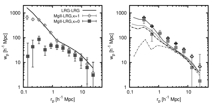
Figure 7.— Left panel: Cross- and auto-correlation results for the 400 $h^{-1}$ Mpc box. The solid line shows the auto-correlation of the mock LRG sample. The diamond points show the cross-correlation results for which $\kappa=1$ for all halos above $10^{12}~{}h^{-1}$ M_⊙. The square points represent the case of no cold gas in the halos of the mock LRGs and $\kappa=1$ for all remaining halos $>10^{12}~{}h^{-1}$ M_⊙. Right panel: the cross- and auto-correlation results for the volume-limited sample of LRGs ($W_{r}(2796)=1-5$ Å) are shown in gray and black points respectively. The four curves correspond to different values of $\kappa$ for the mock LRGs. From bottom to top, $\kappa=0,0.33,0.5,1$.

The presence of cold gas in massive halos has been a debated subject in recent numerical simulation studies. In a series of high-resolution SPH simulations, Keres et al. (2008) and Brooks et al. (2008) examined the temperature history of gas accreted onto dark matter halos. They found that most of the baryonic mass is acquired through filamentary cold mode accretion that is never shock heated to the virial temperature for halos of $\leq 10^{12}$ $h^{-1}\,{\rm M}_{\odot}$. Keres et al. (2008) found that these cold flows are not present in massive halos typically hosting LRGs. At high redshift, cold flows may penetrate inside the virial shock of $10^{13}~{}h^{-1}$ M_⊙, but this effect is highly redshift dependent, and is not likely to yield to cross-correlation functions seen in Figure 4.

Other mechanisms such as thermal instability could generate pockets of cold gas inside a hot medium (e.g., Mo & Miralda-Escude 1996). Maller & Bullock (2004) showed that the hot gas is thermally unstable and prone to fragmentation. They also show that cooling proceeds via the formation of cold $10^{4}$ K clouds in pressure equilibrium with the hot halo gas. For a Milky-Way-size system, cool clouds of mass $\sim 5\times 10^{6}$ $\rm{M}_{\odot}$ are expected to extend up to $\sim 150$ kpc from the galactic center and survive for several Gyrs. Kaufmann et al. (2008) showed that cloud formation is viable in $M_{*}$ halos, but needs to be extended to higher mass. In a similar argument developed by Mo & Miralda-Escude (1996), a two-phase medium in pressure equilibrium was used to explain observations of Lyman limit systems. This model also makes predictions about the presence of C IV around low-mass galaxies and at large impact parameters of massive galaxies. These predictions were partially confirmed later by Chen et al. (2001) who found C IV in galaxies of different morphologies and luminosities. These authors also observed the sharp boundary in the $W_{r}$-(projected separation) plane that was also predicted. Mo & Miralda-Escude (1996) attributed the presence of Mg II absorbers to cold pockets of photoionized gas in halos around massive galaxies. The observed strong Mg II-LRGs cross-correlation signal on scales smaller than the virial radii of halos hosting LRGs indicates the presence of cold gas is more common around massive galaxies than previously thought.

On the observational side, the detections of cool gas in group size halos is uncertain. The challenges lie in the limited sensitivities available to detect HI gas via 21-cm observations (e.g., Verdes-Montenegro et al. 2001, 2007). Verdes-Montenegro et al. (2007) reported detections of HI column density down to $\sim 10^{19}$ cm^-2 in some of the Hickson Compact Groups (Hickson, 1982). Observations are not sensitive enough to probe the low HI column density environment yet.

The difficulty in finding cool gas around groups using 21-cm observations underscores the powerful application of QSO absorption-line studies. We are currently conducting a follow-up imaging and spectroscopy campaign to study the cool gas content of individual LRG halos (Gauthier et al. 2009 in preparation).

5.3. Future prospects : DR7 Mg II database & HOD modeling

Figure 7 demonstrates how a halo occupation approach to the galaxy-absorber cross-correlation function at both large and small scales can put constraints on the covering fraction of cold gas in LRG-hosting dark matter halos. In a forthcoming paper, we will address the detailed halo occupation distribution modeling of the Mg II absorber environment with a particular focus on the one-halo term. This will be achieved by using the SDSS DR7 Mg II absorber catalog. This catalog, currently in preparation (Prochaska et al. 2009), will more than double the number of absorbers from the current DR5 sample. It will allow us to probe smaller projected separations and improve the clustering measurements at $r_{p}<1~{}h^{-1}$ Mpc.

References

- Adelberger et al. (2003) Adelberger, K. L., Steidel, C. C., Shapley, A. E., & Pettini, M. 2003, ApJ, 584, 45
- Bergeron (1986) Bergeron, J. 1986, A&A, 155, L8
- Bergeron & Boissé (1991) Bergeron, J., & Boissé, P. 1991, A&A, 243, 344
- Bergeron & Stasińska (1986) Bergeron, J., & Stasińska, G. 1986, A&A, 169, 1
- Blake et al. (2007) Blake, C., Collister, A., Bridle, S., & Lahav, O. 2007, MNRAS, 374, 1527
- Blake et al. (2008) Blake, C., Collister, A., & Lahav, O. 2008, MNRAS, 385, 1257
- Blanton et al. (2005) Blanton, M. R., et al. 2005, AJ, 129, 2562
- Bond et al. (2001) Bond, N. A., Churchill, C. W., Charlton, J. C., & Vogt, S. S. 2001, ApJ, 562, 641
- Bouché et al. (2004) Bouché, N., Murphy, M. T., & Péroux, C. 2004, MNRAS, 354, L25
- Bouché et al. (2006) Bouché, N., Murphy, M. T., Péroux, C., Csabai, I., & Wild, V. 2006, MNRAS, 371, 495
- Brooks et al. (2008) Brooks, A. M., Governato, F., Quinn, T., Brook, C. B., & Wadsley, J. 2008, ArXiv e-prints
- Brown et al. (2008) Brown, M. J. I., et al. 2008, ApJ, 682, 937
- Cannon et al. (2006) Cannon, R., et al. 2006, MNRAS, 372, 425
- Chen et al. (2001) Chen, H.-W., Lanzetta, K. M., & Webb, J. K. 2001, ApJ, 556, 158
- Chen & Tinker (2008) Chen, H.-W., & Tinker, J. L. 2008, ApJ, 687, 745
- Collister et al. (2007) Collister, A., et al. 2007, MNRAS, 375, 68
- Davis & Peebles (1983) Davis, M., & Peebles, P. J. E. 1983, ApJ, 267, 465
- Dekel et al. (2009) Dekel, A., Sari, R., & Ceverino, D. 2009, ArXiv 0901.2458
- Doyle et al. (2005) Doyle, M. T., et al. 2005, MNRAS, 361, 34
- Eisenstein et al. (2005) Eisenstein, D. J., et al. 2005, ApJ, 633, 560
- Hamilton & Tegmark (2004) Hamilton, A. J. S., & Tegmark, M. 2004, MNRAS, 349, 115
- Hickson (1982) Hickson, P. 1982, ApJ, 255, 382
- Kacprzak et al. (2008) Kacprzak, G. G., Churchill, C. W., Steidel, C. C., & Murphy, M. T. 2008, AJ, 135, 922
- Kaufmann et al. (2008) Kaufmann, T., Bullock, J. S., Maller, A. H., Fang, T., & Wadsley, J. 2008, ArXiv 0812.2025
- Keres et al. (2008) Keres, D., Katz, N., Fardal, M., Dave, R., & Weinberg, D. H. 2008, ArXiv 0809.1430
- Landy & Szalay (1993) Landy, S. D., & Szalay, A. S. 1993, ApJ, 412, 64
- Lanzetta & Bowen (1990) Lanzetta, K. M., & Bowen, D. 1990, ApJ, 357, 321
- Lanzetta & Bowen (1992) Lanzetta, K. M., & Bowen, D. V. 1992, ApJ, 391, 48
- Lundgren et al. (2009) Lundgren, B., & others. 2009, In preparation
- Maller & Bullock (2004) Maller, A. H., & Bullock, J. S. 2004, MNRAS, 471
- Ménard & Chelouche (2008) Ménard, B., & Chelouche, D. 2008, ArXiv 0803.0745
- Ménard et al. (2008) Ménard, B., Nestor, D., Turnshek, D., Quider, A., Richards, G., Chelouche, D., & Rao, S. 2008, MNRAS, 385, 1053
- Mo & Miralda-Escude (1996) Mo, H. J., & Miralda-Escude, J. 1996, ApJ, 469, 589
- Nestor et al. (2007) Nestor, D. B., Turnshek, D. A., Rao, S. M., & Quider, A. M. 2007, ApJ, 658, 185
- Oyaizu et al. (2008) Oyaizu, H., Lima, M., Cunha, C. E., Lin, H., & Frieman, J. 2008, ApJ, 689, 709
- Padmanabhan et al. (2008) Padmanabhan, N., White, M., Norberg, P., & Porciani, C. 2008, ArXiv 0802.210
- Prochter et al. (2006) Prochter, G. E., Prochaska, J. X., & Burles, S. M. 2006, ApJ, 639, 766
- Rao et al. (2006) Rao, S. M., Turnshek, D. A., & Nestor, D. B. 2006, ApJ, 636, 610
- Schneider et al. (2007) Schneider, D. P., et al. 2007, AJ, 134, 102
- Scranton et al. (2003) Scranton, R., et al. 2003, ArXiv astro-ph/0307335
- Spitzer (1956) Spitzer, L. J. 1956, ApJ, 124, 20
- Steidel et al. (1994) Steidel, C. C., Dickinson, M., & Persson, S. E. 1994, ApJ, 437, L75
- Steidel & Sargent (1992) Steidel, C. C., & Sargent, W. L. W. 1992, ApJS, 80, 1
- Sternberg et al. (2002) Sternberg, A., McKee, C. F., & Wolfire, M. G. 2002, ApJS, 143, 419
- Swanson et al. (2008) Swanson, M. E. C., Tegmark, M., Hamilton, A. J. S., & Hill, J. C. 2008, MNRAS, 387, 1391
- Tegmark et al. (2004) Tegmark, M., et al. 2004, Phys. Rev. D, 69, 103501
- Thilker et al. (2004) Thilker, D. A., Braun, R., Walterbos, R. A. M., Corbelli, E., Lockman, F. J., Murphy, E., & Maddalena, R. 2004, ApJ, 601, L39
- Tinker et al. (2008) Tinker, J., Kravtsov, A. V., Klypin, A., Abazajian, K., Warren, M., Yepes, G., Gottlöber, S., & Holz, D. E. 2008, ApJ, 688, 709
- Tinker & Chen (2008) Tinker, J. L., & Chen, H.-W. 2008, ApJ, 679, 1218
- Tinker et al. (2007) Tinker, J. L., Norberg, P., Weinberg, D. H., & Warren, M. S. 2007, ApJ, 659, 877
- Tinker et al. (2005) Tinker, J. L., Weinberg, D. H., Zheng, Z., & Zehavi, I. 2005, ApJ, 631, 41
- Tinker et al. (2009) Tinker, J. L., & others. 2009, In preparation
- van Zee et al. (1998) van Zee, L., Salzer, J. J., & Haynes, M. P. 1998, ApJ, 497, L1+
- Verdes-Montenegro et al. (2007) Verdes-Montenegro, L., Yun, M. S., Borthakur, S., Rasmussen, J., & Ponman, T. 2007, New Astronomy Review, 51, 87
- Verdes-Montenegro et al. (2001) Verdes-Montenegro, L., Yun, M. S., Williams, B. A., Huchtmeier, W. K., Del Olmo, A., & Perea, J. 2001, A&A, 377, 812
- Wake et al. (2008) Wake, D. A., et al. 2008, MNRAS, 387, 1045
- Wang (1993) Wang, B. 1993, ApJ, 415, 174
- Weiner et al. (2008) Weiner, B. J., et al. 2008, ArXiv 0804.4686
- York et al. (2000) York, D. G., et al. 2000, AJ, 120, 1579
- Zaritsky et al. (1994) Zaritsky, D., Kennicutt, R. C., & Huchra, J. P. 1994, ApJ, 420, 87
- Zehavi et al. (2004) Zehavi, I., et al. 2004, ApJ, 608, 16
- Zehavi et al. (2005) —. 2005, ApJ, 630, 1
- Zheng (2004) Zheng, Z. 2004, ApJ, 610, 61
- Zheng et al. (2007) Zheng, Z., Coil, A. L., & Zehavi, I. 2007, ApJ, 667, 760
- Zheng et al. (2008) Zheng, Z., Zehavi, I., Eisenstein, D. J., Weinberg, D. H., & Jing, Y. 2008, ArXiv 0809.1868
- Zibetti et al. (2007) Zibetti, S., Ménard, B., Nestor, D. B., Quider, A. M., Rao, S. M., & Turnshek, D. A. 2007, ApJ, 658, 161