Dispersive interactions between atoms and non planar surfaces

Abstract

We calculate the dispersive force between a ground state atom and a non planar surface. We present explicit results for a corrugated surface, derived from the scattering approach at first order in the corrugation amplitude. A variety of analytical results are derived in different limiting cases, including the van der Waals and Casimir-Polder regimes. We compute numerically the exact first-order dispersive potential for arbitrary separation distances and corrugation wavelengths, for a Rubidium atom on top of a silicon or gold corrugated surface. We discuss in detail the inadequacy of the proximity force approximation, and present a simple but adequate approximation for computing the potential.

I Introduction

Quantum and thermal fluctuations of the electromagnetic field in the presence of material boundaries generate fluctuating spatial gradients of the field intensity and fluctuating induced electric dipoles in ground-state atoms close to those surfaces, resulting in an atom-surface interaction via the optical dipole force. These dispersive forces have considerable importance in fundamental physics, including deflection of atomic beams close to surfaces deflection , classical Aspect1996 and quantum reflection of cold atoms Shimizu2001 ; DeKieviet2003 and Bose-Einstein condensates (BECs) QRbec from surfaces, dipole oscillations of BECs above dielectric surfaces Cornell05 ; Cornell07 , and in possible future applications of single-atom manipulation in atom chips atomchip ; CAMS05 . At the limit of large separation distances (Casimir-Polder limit CasimirPolder ), the interactions show universal features since they depend only on the zero-frequency atom and surface optical responses.

Dispersive forces can be tailored in different ways, either by engineering the optical properties of the surfaces Buhmann07 ; Rosa08 ; Pitaevskii08 , by biasing the temperatures of the surfaces and their thermal environment Cornell07 ; Antezza05 ; Buchleitner08 , or by suitably changing their geometry. Given the complexity of these quantum forces, which arise from fluctuations at all frequency and length scales, calculations beyond planar geometries are exceedingly involved. Until recently, approximate methods have been used to deal with non-planar setups, including the proximity force approximation (PFA) Derjaguin57 and the pairwise summation approach (PWS) Galina00 . However, these approximate methods drastically fail when the surface is not sufficiently smooth on the length-scale of the atom-surface separation, since they do not properly take into account the non-additivity of dispersion forces JPA . These large deviations from PFA or PWS could be probed by using present-day technology, for example with a Bose-Einstein condensate above a microfabricated corrugated surface PRL . Similar deviations have been recently measured for the Casimir force between a metallic sphere and a nanostructured silicon rectangular grating Chan08 ; Lambrecht08 .

A number of methods are available to compute the dispersive atom-surface forces (see for example CasimirPolder ; Barton ; WylieSipe ; Mostepanenko ; Buhman05 ). These methods allow the exact computation of the force for very simple geometries, such as an atom above a single (possibly multilayered) plane, sphere or cylinder, or an atom inside a plane Fabry-Perot cavity. Toy models with scalar fields with ideal (Dirichlet) boundary conditions have also been considered to compute the “scalar Casimir-Polder” force for a small sphere above a uni-axial corrugated surface Gies08 .

Similar problems have been discussed for the Casimir interaction between two macroscopic bodies (see for example Lifshitz56 ; DLP ; Kats77 ), and the scattering approach has been shown to be a very efficient tool for analyzing the case of non-trivial geometries Lambrecht06 . For parallel plates, the Casimir force may be written in terms of the reflection coefficients seen from the region in-between the plates JaekelReynaud91 ; Genet2003 . A similar expression also holds for non-planar surfaces, with the specular reflection coefficients replaced by more general reflection operators that describe non-specular diffraction by the surfaces. This allows for the computation of the Casimir force between rough MaiaNeto05 or corrugated Rodrigues06 surfaces. Similar methods have been employed to compute the force between a plane and a sphere Bulgac06 ; Bordag06 ; Emig08 ; MaiaNeto08 and between two spheres Emig07 ; Kenneth08 .

In this paper we develop the scattering approach for studying the dispersive interaction between ground-state atoms and arbitrarily shaped surfaces characterized by frequency-dependent reflection operators. This approach provides an exact analytical expression for the two-body interaction energy, which can be written in terms of the scattering matrices defined for each individual, one-body, scatterer. Although this is a simpler problem than solving for the many-body Green function, it is still very difficult to find the exact scattering matrices for the problem of a electromagnetic field impinging on a given non-planar geometry. In order to illustrate the method, we write the two-body interaction energy in a perturbative expansion in terms of the deviation of the surface profile from the planar case PRL . Apart from this perturbative approximation, the approach is valid for any value of the corrugation wavelength and includes the full electromagnetic fluctuations and the real material properties of the boundaries. We compute the perturbative dispersive interaction potential to first order in the surface profile both for ideal and real materials, and discuss the prospects of measuring non-trivial (beyond PFA) geometrical effects with a uni-axial corrugated surface interacting with a Bose-Einstein condensate used as a vacuum field sensor.

The paper is organized in the following way. In Sec. 2, we develop the scattering formalism for the atom-surface interaction. The resulting general formula is then applied to calculate the potential to first order in the surface corrugation amplitude in Sec. 3. We compare our results with PFA in Sec. 4 and discuss experimental prospects in Sec. 5. Concluding remarks are presented in Sec. 6.

II Atom-surface interaction for non-planar geometries

We consider a ground-state atom at position ${\bf R}_{A}=(\mathbf{r}_{A},z_{A})$ on top of a non-planar surface, as shown by Fig. 1. The surface profile is defined by the function $h(x,y)$ representing the local height with respect to the plane $z=0.$ The atom is in free space, so that $z_{A}>h(\mathbf{r}_{A}).$ The fluctuating electromagnetic field propagating from the surface towards the atom is written in the mixed Fourier representation (frequency $\omega$, two-dimensional wave vector ${\bf k}$)

$${\bf E}^{\uparrow}({\bf k},z,\omega)=\sum_{p=\mathrm{TE},\mathrm{TM}}{E}_{p}^{\uparrow}({\bf k},\omega)\mbox{\boldmath${\hat{\epsilon}}$}^{+}_{p}({\bf k},\omega)e^{ik_{z}z},$$ (1)

where $p$ is the polarization index and $k_{z}$ the longitudinal wavevector (sgn denotes the sign function; $k=|\mathbf{k}|$)

$$k_{z}={\rm sgn}(\omega)\sqrt{\omega^{2}/c^{2}-k^{2}}.$$

Similar expressions in terms of unit vectors $\mbox{\boldmath${\hat{\epsilon}}$}^{-}_{\scriptstyle\rm TE}$ and $\mbox{\boldmath${\hat{\epsilon}}$}^{-}_{\scriptstyle\rm TM}$ hold for the field ${\bf E}^{\downarrow}({\bf k},z,\omega)$ propagating towards the surface, with the replacement $k_{z}\rightarrow-k_{z}$. The complete wave vector is denoted as ${\bf K}^{\pm}={\bf k}\pm k_{z}\mathbf{\hat{z}}$, and the unit vectors given by (the frequency dependence will be generally omitted)

$$\mbox{\boldmath${\hat{\epsilon}}$}^{+}_{\scriptstyle\rm TE}({\bf k}) =\mbox{\boldmath${\hat{\epsilon}}$}^{-}_{\scriptstyle\rm TE}({\bf k})=\mathbf{\hat{z}}\times\mathbf{\hat{k}},$$

$$\mbox{\boldmath${\hat{\epsilon}}$}^{\pm}_{\scriptstyle\rm TM}({\bf k}) =\mbox{\boldmath${\hat{\epsilon}}$}^{\pm}_{\scriptstyle\rm TE}({\bf k})\times\mathbf{\hat{K}}^{\pm},$$

correspond to transverse electric (TE) and magnetic (TM) polarizations, respectively.

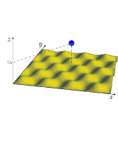
Figure 1: (color online) Ground-state atom on top of a non-planar surface (profile function $h(x,y)$).

The reflection by the non-planar surface modifies the wave vector $\bf k$ and the polarization $p={\rm TE,TM}$, while conserving the frequency $\omega$ since the surface is assumed to be stationary

$${E}^{\uparrow}_{p}({\bf k},\omega)=\int\frac{d^{2}{\bf k}^{\prime}}{(2\pi)^{2}}\sum_{p^{\prime}}\langle{\bf k},p|{\cal R}_{S}(\omega)|{\bf k}^{\prime},p^{\prime}\rangle\;{E}^{\downarrow}_{p^{\prime}}({\bf k}^{\prime},\omega).$$ (2)

The reflection operator ${\cal R}_{S}(\omega)$ depends on the surface profile function $h(x,y)$. Explicit results for its matrix elements are presented in Sec. 3 to first order in $h(x,y)$.

Let us assume for a moment that the $z$-axis is taken along the atom position ($\mathbf{r}_{A}={\bf 0}$). At zero temperature, the Casimir atom-surface interaction energy is then given by the zero-temperature scattering formula as an integral over the positive imaginary frequency axis ($\omega\rightarrow i\xi$) Lambrecht06

$$U({\bf R}_{A})=\hbar\,\int_{0}^{\infty}\frac{d\xi}{2\pi}{\rm Tr}\log\left(1-{\cal R}_{S}\,\,e^{-{\cal K}z_{A}}\,{\cal R}_{A}\,e^{-{\cal K}z_{A}}\right),$$

$${\cal K}={\rm diag}(\kappa)\;,\quad\kappa=\sqrt{\xi^{2}/c^{2}+k^{2}}$$ (3)

with ${\cal R}_{A}$ and ${\cal R}_{S}$ representing the reflection operators for the atom and the surface, respectively. ${\cal K}$ is a diagonal operator in the basis of plane waves $|\mathbf{k},p\rangle$ with eigenvalues $\kappa$, so that $e^{-{\cal K}z_{A}}$ represents the propagation between the two scatterers. Alternatively, it may also be interpreted as the displacement operator Emig07 : here ${\cal R}_{A}$ is computed for a coordinate axis centered at the atom center-of-mass, whereas $e^{-{\cal K}z_{A}}\,{\cal R}_{A}\,e^{-{\cal K}z_{A}}$ corresponds to the ‘laboratory’ axis. A similar expression holds at finite temperature, replacing the integral over imaginary frequencies $\xi$ by a sum over Matsubara frequencies.

It is actually simple to calculate the atomic reflection operator for an arbitrary position $(\mathbf{r}_{A},z_{A})$ when taking the plane wave basis. The spherically-symmetric ground-state atom is described as an induced electric dipole, with a dipole moment

$${\bf d}(\omega)=\alpha(\omega){\bf E}({\bf R}_{A},\omega).$$ (4)

Let us emphasize at this point that $\alpha(\omega)$ is the dynamic polarizability defined according to SI unit system esucgs . The dipole field components in the region $z<z_{A}$ are written in the representation defined by (1) with Carminati98

$${E}^{\downarrow}_{({\rm dip})p}({\bf k},\omega)=\frac{i\omega^{2}}{2\epsilon_{0}c^{2}k_{z}}\,\mbox{\boldmath${\hat{\epsilon}}$}^{-}_{p}(\mathbf{k})\cdot{\bf d}(\omega)e^{-i\mathbf{k}\cdot\mathbf{r}_{A}}e^{ik_{z}z_{A}}.$$ (5)

When replacing (4) into (5), we find two separate contributions associated to the field Fourier components propagating upwards or downwards. To calculate the atom reflection operator, we take the upward components

$${E}^{\downarrow}_{({\rm dip})p}({\bf k},\omega)=\frac{i\omega^{2}\,\alpha(\omega)}{2\epsilon_{0}c^{2}k_{z}}\,\int\frac{d^{2}{\bf k}^{\prime}}{(2\pi)^{2}}\sum_{p^{\prime}}\mbox{\boldmath${\hat{\epsilon}}$}^{-}_{p}(\mathbf{k})\cdot\mbox{\boldmath${\hat{\epsilon}}$}^{+}_{p^{\prime}}(\mathbf{k}^{\prime})$$

$$\times e^{-i(\mathbf{k}-\mathbf{k}^{\prime})\cdot\mathbf{r}_{A}}e^{i(k_{z}+k_{z}^{\prime})z_{A}}{E}^{\uparrow}_{p^{\prime}}({\bf k}^{\prime},\omega).$$ (6)

This result can be cast into a form similar to (2), with the atomic reflection operator given by ($\omega\rightarrow i\xi$ and $k_{z}\rightarrow i\kappa$)

$$\langle\mathbf{k},p|{\cal R}_{A}|\mathbf{k}^{\prime},p^{\prime}\rangle = -\frac{{\xi}^{2}}{2\kappa}\frac{\alpha(i\xi)}{\epsilon_{0}c^{2}}\hat{\epsilon}_{p}^{-}(\mathbf{k})\cdot\hat{\epsilon}_{p^{\prime}}^{+}(\mathbf{k}^{\prime})$$ (7)

$$\times e^{-i(\mathbf{k}-\mathbf{k}^{\prime})\cdot\mathbf{r}_{A}}e^{-(\kappa+\kappa^{\prime})z_{A}}.$$

The dependence on $\mathbf{r}_{A}$ and $z_{A}$ in this equation is exactly the one expected from the matrix elements of the displacement operator in the plane wave basis. The displacement along the $z$-axis was already explicitly taken into account in the scattering formula (II), so we must take $z_{A}=0$ when replacing (7) into (II).

As we assume that the atom-surface separation distance is much larger than the atomic dimensions, we may expand the general scattering formula (II) to first order in $\alpha(\omega)$ or, equivalently, to first order in ${\cal R}_{A}$ foot_linear-alpha

$$U({\bf R}_{A}) = -\hbar\int_{0}^{\infty}\frac{d\xi}{2\pi}\int\frac{d^{2}{\bf k}}{(2\pi)^{2}}\int\frac{d^{2}{\bf k}^{\prime}}{(2\pi)^{2}}e^{-(\kappa+\kappa^{\prime})z_{A}}$$ (8)

$$\times \sum_{p,p^{\prime}}\langle{\bf k},p|{\cal R}_{S}|{\bf k}^{\prime},p^{\prime}\rangle\langle{\bf k}^{\prime},p^{\prime}|{\cal R}_{A}|{\bf k},p\rangle.$$

The $z_{A}$ dependence is already explicit in (8) because ${\cal R}_{A}$ in (II) was defined with respect to reference axis such that $z_{A}=0.$ Note that the resulting $z_{A}$ dependence coincides with (7), which was derived for an arbitrary position with respect to the origin. From (7) and (8), we find

$$U({\bf R}_{A})=\frac{\hbar}{\epsilon_{0}c^{2}}\int_{0}^{\infty}\frac{d\xi}{2\pi}\xi^{2}\alpha(i\xi)\int\frac{d^{2}{\bf k}}{(2\pi)^{2}}\int\frac{d^{2}{\bf k}^{\prime}}{(2\pi)^{2}}$$

$$\times\frac{e^{i({\bf k}-{\bf k}^{\prime})\cdot{\bf r}_{A}}e^{-(\kappa+\kappa^{\prime})z_{A}}}{2\kappa^{\prime}}$$ (9)

$$\times\sum_{p,p^{\prime}}\langle{\bf k},p|{\cal R}_{S}|{\bf k}^{\prime},p^{\prime}\rangle\;\mbox{\boldmath${\hat{\epsilon}}$}^{+}_{p}({\bf k})\cdot\mbox{\boldmath${\hat{\epsilon}}$}^{-}_{p^{\prime}}({\bf k}^{\prime}).$$

Note that this general formula holds for magneto-dielectric media, including the anisotropic case Rosa08 . The dispersive potential for an atom with magnetic polarizability Feinberg can also be derived from (II) along the lines presented above. The corresponding atomic reflection operator is calculated in Appendix A.

As a first application of (II), we briefly consider the case of a planar surface at $z=0$ (corresponding to a profile function $h(x,y)=0$) made of some isotropic material. In this case, ${\cal R}_{S}$ is diagonal, its matrix elements being

$$\langle{\bf k},p|{\cal R}_{S}|{\bf k}^{\prime},p^{\prime}\rangle=(2\pi)^{2}\delta^{(2)}({\bf k}-{\bf k}^{\prime})\delta_{p,p^{\prime}}r^{p}(k,i\xi),$$ (10)

where $r^{p}(k,i\xi)$ are the specular reflection coefficients for the plane surface. For instance, for a homogeneous non-magnetic bulk medium, they are given by the Fresnel formulas ($\epsilon(i\xi)=$ electric permittivity)

$$r^{\rm TE}({\bf k},i\xi)=\frac{\kappa-\kappa_{t}}{\kappa+\kappa_{t}}\,,\;r^{\rm TM}({\bf k},i\xi)=\frac{\epsilon(i\xi)\kappa-\kappa_{t}}{\epsilon(i\xi)\kappa+\kappa_{t}},$$

$$\kappa_{t}=\sqrt{k^{2}+\epsilon(i\xi)\xi^{2}/c^{2}}$$ (11)

Eq. (II) then yields the known interaction energy between a ground-state atom and a plane surface valid for arbitrary separation distances Barton ; WylieSipe ; Mostepanenko ; DLP ; Buhman05

$$U^{(0)}(z_{A}) = \frac{\hbar}{\epsilon_{0}c^{2}}\,\int_{0}^{\infty}\frac{d\xi}{2\pi}\,\xi^{2}\alpha(i\xi)\int\frac{d^{2}\mathbf{k}}{(2\pi)^{2}}\,\frac{e^{-2\kappa z_{A}}}{2\kappa}$$

$$\times\left[r^{\mathrm{TE}}(\mathbf{k},i\xi)-\Bigl{(}1+\frac{2c^{2}k^{2}}{\xi^{2}}\Bigr{)}r^{\mathrm{TM}}(\mathbf{k},i\xi)\right].$$

This expression can be simplified under the assumption of small or large distances $z_{A}$ (with respect to some typical atomic transition wavelength $\lambda_{A}$). For $z_{A}\ll\lambda_{A}$ and $z_{A}\gg\lambda_{A}$, we get the van der Waals and Casimir-Polder limits which correspond respectively to Eqs. (24) and (22) in Ref. Antezza04 .

Eq. (II) represents a general result for the dispersive interaction between an atom and a body scatterer. The difficulty, of course, lies in the explicit derivation of the matrix elements of the corresponding operator ${\cal R}_{S}$. In the next section, we apply this result to derive the lateral dispersive force for an atom on top of a corrugated surface up to first order in the corrugation profile $h(\mathbf{r})$. A second interesting application, left for a future publication, would be to compute the roughness correction to the normal dispersive force – in this case it is necessary to compute ${\cal R}_{S}$ up to second order in $h(\mathbf{r})$ (see MaiaNeto05 ).

III Perturbative interaction potential within the scattering approach

In order to compute the exact atom-surface interaction potential it is necessary to find the reflection operators of the surface, which is a highly non-trivial problem. For the sake of illustration of the scattering formalism applied to the atom-surface problem, we now compute those reflection operators in a perturbative expansion in terms of the deviations $h({\bf r})$ of the surface profile with respect to the planar configuration. We will calculate the atom-surface interaction energy to first order in $h$. This term gives rise both to a correction to the normal force and to a lateral force on the atom which does not exist in the case of a planar surface. We start by expanding the reflection operators in powers of $h$ as ${\cal R}={\cal R}^{(0)}+{\cal R}^{(1)}+O(h^{2})$. We model the optical response of the homogeneous isotropic material in terms of its frequency-dependent electric permittivity $\epsilon(i\xi)$. The zeroth-order term ${\cal R}^{(0)}$ is given by (10), whereas the first-order reflection matrix elements can be written as

$$\langle{\bf k},p|{\cal R}^{(1)}|{\bf k}^{\prime},p^{\prime}\rangle=R^{(1)}_{pp^{\prime}}({\bf k},{\bf k}^{\prime})H({\bf k}-{\bf k}^{\prime}),$$ (13)

where $H({\bf k})$ is the Fourier transform of the surface profile $h({\bf r})$. Therefore, the first-order atom-surface interaction potential is

$$U^{(1)}({\bf R}_{A})=\int\frac{d^{2}{\bf k}}{(2\pi)^{2}}e^{i{\bf k}\cdot{\bf r}_{A}}g(\mathbf{k},z_{A})H({\bf k}),$$ (14)

where $g(\mathbf{k},z_{A})$ is the response function

$$g(\mathbf{k},z_{A}) =\frac{\hbar}{\epsilon_{0}c^{2}}\int_{0}^{\infty}\frac{d\xi}{2\pi}\xi^{2}\alpha(i\xi)\int\frac{d^{2}{\bf k}^{\prime}}{(2\pi)^{2}}a_{{\bf k}^{\prime},{\bf k}^{\prime}-{\bf k}}$$

$$a_{{\bf k}^{\prime},{\bf k}^{\prime\prime}} =\frac{e^{-(\kappa^{\prime}+\kappa^{\prime\prime})z_{A}}}{2\kappa^{\prime\prime}}$$

$$\times\sum_{p^{\prime},p^{\prime\prime}}\hat{\mbox{\boldmath$\epsilon$}}^{+}_{p^{\prime}}({\bf k}^{\prime})\cdot\hat{\mbox{\boldmath$\epsilon$}}^{-}_{p^{\prime\prime}}({\bf k}^{\prime\prime})R^{(1)}_{p^{\prime}p^{\prime\prime}}({\bf k}^{\prime},{\bf k}^{\prime\prime}).$$

The first-order reflection matrix was calculated in MaiaNeto05 by following the approach presented in Greffet88 (see also Agarwal ). It is a non-diagonal matrix with non-specular reflection coefficients given by

$$R^{(1)}_{pp^{\prime}}({\bf k},{\bf k}^{\prime})=u_{pp^{\prime}}(k,k^{\prime};i\xi)\,\Lambda_{pp^{\prime}}^{(1)}({\bf k},{\bf k}^{\prime};i\xi),$$ (16)

where we have defined

$$u_{pp^{\prime}}(k,k^{\prime};i\xi)=\frac{r^{p}(k,i\xi)t^{p^{\prime}}(k^{\prime},i\xi)}{t^{p}(k,i\xi)}.$$ (17)

$t^{p}({\bf k},i\xi)$ are the transmission Fresnel coefficients for the planar interface defined by

$$t^{\rm TE}({\bf k},i\xi)=\frac{2\kappa}{\kappa+\kappa_{t}} t^{\rm TM}({\bf k},i\xi)=\frac{2\sqrt{\epsilon(i\xi)}\kappa}{\epsilon(i\xi)\kappa+\kappa_{t}}.$$ , (18)

The matrix ${\bf\Lambda}^{(1)}$ is expressed as ${\bf\Lambda}^{(1)}={\bf\Lambda}^{(1)}_{+}-{\bf\Lambda}^{(1)}_{-}$ with

$${\bf\Lambda}^{(1)}_{\pm}({\bf k},{\bf k}^{\prime};i\xi)=(\kappa_{t}\pm\kappa){\bf B}^{-1}_{t}\left(\begin{array}[]{cc}C&S\\ -\frac{S}{1\pm\beta\beta_{t}}&\frac{C\pm\beta\beta^{\prime}_{t}}{1\pm\beta\beta_{t}}\end{array}\right){\bf B}^{\prime}_{t},$$ (21)

$${\bf B}_{t}={\rm diag}(1,c\kappa_{t}/\sqrt{\epsilon(i\xi)}\xi),\quad\beta=k/\kappa,\quad\beta_{t}=k/\kappa_{t},$$

$$C=\cos(\phi-\phi^{\prime}),\quad S=\sin(\phi-\phi^{\prime}).$$ (22)

We have denoted with $\phi$ ($\phi^{\prime}$) the angle between $\mathbf{k}$ ($\mathbf{k}^{\prime}$) and an arbitrarily chosen axis on the surface plane. Starting from these definitions and using the scalar product of polarization vectors

$$\hat{\mbox{\boldmath$\epsilon$}}^{+}_{\rm TE}({\bf k})\cdot\hat{\mbox{\boldmath$\epsilon$}}^{-}_{\rm TE}({\bf k}^{\prime}) = C,$$

$$\hat{\mbox{\boldmath$\epsilon$}}^{+}_{\rm TE}({\bf k})\cdot\hat{\mbox{\boldmath$\epsilon$}}^{-}_{\rm TM}({\bf k}^{\prime}) = \frac{c\kappa^{\prime}S}{\xi},$$

$$\hat{\mbox{\boldmath$\epsilon$}}^{+}_{\rm TM}({\bf k})\cdot\hat{\mbox{\boldmath$\epsilon$}}^{-}_{\rm TE}({\bf k}^{\prime}) = \frac{c\kappa S}{\xi},$$

$$\hat{\mbox{\boldmath$\epsilon$}}^{+}_{\rm TM}({\bf k})\cdot\hat{\mbox{\boldmath$\epsilon$}}^{-}_{\rm TM}({\bf k}^{\prime}) = -\frac{c^{2}}{\xi^{2}}(kk^{\prime}+\kappa\kappa^{\prime}C),$$ (23)

we obtain for $a_{{\bf k}^{\prime},{\bf k}^{\prime\prime}}$ the following general expression

$$a_{{\bf k}^{\prime},{\bf k}^{\prime\prime}}=e^{-(\kappa^{\prime}+\kappa^{\prime\prime})z_{A}}\frac{\kappa^{\prime}}{\kappa^{\prime\prime}}\left[C^{2}u_{\rm TE,TE}+\frac{\kappa^{\prime\prime}\kappa^{\prime\prime}_{t}S^{2}}{\sqrt{\epsilon(i\xi)}\xi^{2}/c^{2}}u_{\rm TE,TM}\right.$$

$$\left.+\frac{\sqrt{\epsilon(i\xi)}\kappa^{\prime}\kappa^{\prime}_{t}S^{2}}{\xi^{2}/c^{2}-(\kappa^{\prime})^{2}[\epsilon(i\xi)+1]}u_{\rm TM,TE}+\frac{[k^{\prime}k^{\prime\prime}+\kappa^{\prime}\kappa^{\prime\prime}C][\epsilon(i\xi)k^{\prime}k^{\prime\prime}+\kappa^{\prime}_{t}\kappa^{\prime\prime}_{t}C]}{(\xi^{2}/c^{2})\{\xi^{2}/c^{2}-(\kappa^{\prime})^{2}[\epsilon(i\xi)+1]\}}u_{\rm TM,TM}\right].$$ (24)

By inspection of Eq. (24), one shows that the response function $g(\mathbf{k},z_{A})$ depends only on the modulus $k=|{\bf k}|$ of the corrugation wave vector, as expected: the information about the direction associated to the surface profile is contained only in $H({\bf k})$, whereas the response function derived within the perturbative approach is based on the planar geometry and its underlying symmetry.

The results presented above allow for the numerical calculation of the first-order potential for arbitrary ground-state atoms and material media by plugging the corresponding polarizability and permittivity functions into Eqs. (III) and (24). As an illustration, we consider a ground-state rubidium atom above a gold or a silicon surface. The dynamical atomic polarizability is obtained from Babb , and optical data for gold and silicon are obtained from Palik . The values along the imaginary frequency axis are then calculated with the help of dispersion relations Lambrecht00 ; Lambrecht04 .

In Fig. 2, we plot the response function after normalizing it by

$$F_{\rm CP}^{(0)}(z_{A})=-\frac{3\hbar c\alpha(0)}{8\pi^{2}\epsilon_{0}\,z_{A}^{5}},$$ (25)

that is also the result derived by Casimir and Polder CasimirPolder for the attractive force on an atom on top of a perfectly-reflecting plate at large separation distances. The horizontal axis represents the atom-surface separation $z_{A}$. We take two different values of $k,$ corresponding to corrugation wavelengths $\lambda=2\pi/k=10\,\mu{\rm m}$ and $100\,{\rm nm}.$

The global shape of the curves can be discussed in a qualitative manner, which will be made more quantitative later on. At low values of $kz_{A}$, PFA is expected to hold so that the response is approximately independent of $k.$ The ratio $g(k,z_{A})/F_{\rm CP}$ thus grows linearly with $z,$ showing the well-known power-law change when sweeping from the unretarded van der Waals to the Casimir-Polder regime. As $z_{A}$ approaches $1/k,$ PFA becomes gradually worse, and then a nontrivial geometry effect reduces $g(k,z_{A})$ exponentially for $z_{A}\gg 1/k.$ In the next section, we show that geometry and real material effects can be disentangled in most cases of interest, thus providing a simple manner to explain how they jointly produce the results shown in Fig. 2.

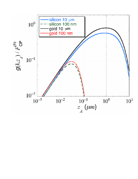
Figure 2: (color online) Dimensionless ratio $g(k,z_{A})/F_{\rm CP}^{(0)}(z_{A})$ as a function of separation distance $z_{A}$ (for a ground-state Rb atom). For the corrugation wavelength $\lambda=2\pi/k=10\,\mu{\rm m},$ we show the values for gold (black) and silicon (blue) surfaces. We also show the results for $\lambda=100\,{\rm nm}$ with gold (dotted red) and silicon (dashed green) surfaces.

IV Disentangling geometry and real material effects

As discussed in the Introduction, the most commonly used approximation methods to compute atom-surface interactions are the proximity force approximation (PFA) and pairwise summation approach (PWS). In JPA we compared these approximate methods with our exact scattering approach to first-order in the surface profile for the case of perfect reflectors, and showed that PFA overestimates and PWS underestimates the lateral atom-surface force. In this section we want to expand upon these considerations and consider in further detail the corrections to the PFA approximation beyond the case of perfect reflection. This will allow us to disentangle the effects of geometry and real materials, thus leading to a very simple rule for the evaluation of $g(k,z_{A}).$

In the atom-surface context, the proximity force approximation amounts to compute the atom-surface potential $U$ for a given geometry from the potential for the planar geometry $U^{(0)}$ taken at the local atom-surface distance

$$U\simeq U^{(0)}(z_{A}-h({\bf r}_{A}))\simeq U^{(0)}-h({\bf r}_{A})\partial_{z}U^{(0)}.$$

The PFA holds when the surface is very smooth in the scale of the separation distance, that is in the limit $kz_{A}\rightarrow 0$. From our expression for the first-order potential (14) one can indeed prove that for any material the response function satisfies the “proximity force theorem”

$$g(k=0,z_{A})=-\partial_{z}U^{(0)}(z_{A}).$$ (26)

This follows from the fact that the response function at zero transverse momentum is given by the specular limit of the non-specular coefficients $a_{{\bf k}^{\prime},{\bf k}^{\prime\prime}}$, which corresponds to ${\bf k}^{\prime}={\bf k}^{\prime\prime}$. In this case we have $R^{(1)}_{p^{\prime},p^{\prime\prime}}({\bf k}^{\prime},{\bf k}^{\prime})=2\kappa^{\prime}r^{p^{\prime}}({\bf k}^{\prime};i\xi)\delta_{p^{\prime},p^{\prime\prime}}$, and $a_{{\bf k}^{\prime},{\bf k}^{\prime}}=e^{-2\kappa z_{A}}\sum_{p^{\prime}}\hat{\mbox{\boldmath$\epsilon$}}^{+}_{p^{\prime}}({\bf k}^{\prime})\cdot\hat{\mbox{\boldmath$\epsilon$}}^{-}_{p^{\prime}}({\bf k}^{\prime})r^{p^{\prime}}({\bf k}^{\prime};i\xi)$. From (III), the zero-momentum response function is then

$$g(k=0,z_{A})=\frac{\hbar}{\epsilon_{0}c^{2}}\int_{0}^{\infty}\frac{d\xi}{2\pi}\xi^{2}\alpha(i\xi)$$

$$\times\int\frac{d^{2}{\bf k}}{(2\pi)^{2}}e^{-2\kappa z_{A}}\sum_{p}\hat{\mbox{\boldmath$\epsilon$}}^{+}_{p}({\bf k})\cdot\hat{\mbox{\boldmath$\epsilon$}}^{-}_{p}({\bf k})r^{p}({\bf k};i\xi).$$ (27)

Comparing with expression (II) for $U^{(0)}$, we immediately prove the proximity force theorem (26).

As a consequence of this discussion, we recover (IV) from our more general result (14) when replacing $g(k,z_{A})$ by $g(0,z_{A}).$ Now the value of $g(k,z_{A})$ differs from $g(0,z_{A})$ for any finite value of $k$ and it is worth quantifying deviations from PFA by introducing the function

$$\rho(k,z_{A})=\frac{g(k,z_{A})}{g(0,z_{A})}.$$ (28)

Deviations from PFA can first be discussed in the vicinity of $k=0$ where PFA is recovered ($\rho\rightarrow 1$ for $k\rightarrow 0$). It is possible to deduce from (III)-(24) that the first order derivative of $\rho$ with respect to $k$ is identically zero, for any atomic polarizability and surface permittivity. It follows that deviations from PFA appear only at order $k^{2}$ in a Taylor expansion around $k=0$

$$\rho(k,z_{A})=1+\frac{k^{2}}{2}\partial_{k}^{2}\rho(0,z_{A})+O(k^{3}).$$ (29)

For perfect reflectors, we can also prove that the second-order derivative in (29) is negative, so that $\rho(k,z_{A})$ is concave near $k=0.$

When going far beyond PFA (arbitrary values of $kz_{A}$), we have to compute $\rho(k,z_{A})$ numerically. The result of this calculation is plotted on Fig. 3, with $\rho$ shown as a function of $kz_{A}$ for three different values of $z_{A}$ in the case of an Rb atom on top of a Si surface. We notice that these curves are quite close to one another. In order to obtain an estimate of their values, we also show the curve corresponding to the Casimir-Polder limit for perfect reflectors, which is derived from (28) and the calculations of Appendix B

$$\rho_{\rm CP}^{\rm perf}(k,z_{A})=e^{-kz_{A}}\left(1+kz_{A}+\frac{16(kz_{A})^{2}}{45}+\frac{(kz_{A})^{3}}{45}\right).$$ (30)

For this limiting case, $\rho$ depends only on the dimensionless ${\cal Z}=kz_{A}$. We may thus conclude that this variable captures most of the geometry correction, since $\rho$ depends very little on $z_{A}$ for a given ${\cal Z}.$ For distances larger than $1\,\mu{\rm m}$, $\rho$ may be well approximated by the CP formula Eq. (30). This statement holds for the case of silicon, but the results for gold surfaces (not shown) are even closer to the CP curve shown in Fig. 3.

Of course, finite conductivity corrections are very important for the evaluation of the force between an atom and a plane plate, and the full response function $g$ has to be written as

$$g(k,z)=\rho(k,z)\,\eta_{F}\,F^{(0)}_{\rm CP}$$ (31)

In this formula, $F^{(0)}_{\rm CP}$ is the Casimir-Polder force (25), $\eta_{F}=F^{(0)}/F^{(0)}_{\rm CP}$ represents the reduction of the dispersive force due to material properties of atom and surface (calculated for a plane geometry), and $\rho$ describes the effect of geometry.

In Fig. 4, we plot $\eta_{F}$ as a function of $z_{A}$ for a Rb atom on top of a silicon or gold surface. As expected, the CP result for perfect reflectors is recovered at large distances in the case of gold, whereas for silicon we find a reduction of $\eta_{F}\sim 2/3$ due to the finite value of the zero-frequency permittivity in this case. These results coincide with those obtained in Antezza04 . For both gold and silicon surfaces, the reduction gets stronger as the separation distance is decreased, as expected since shorter distances correspond to larger frequencies, for which the optical responses of both atom and surface are smaller. For very short distances, $\eta_{F}$ is linear ($\eta_{F}\approx 5.8\,z(\mu{\rm m})$ for gold and $5.1\,z(\mu{\rm m})$ for silicon), in agreement with the power law modification expected in the van der Waals unretarded regime.

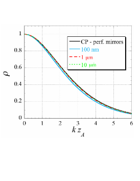
Figure 3: (color online) Geometry correction factor $\rho$ as a function of $kz_{A}$ for a silicon surface and $z_{A}=100\,{\rm nm}$ (light blue), $1\,\mu{\rm m}$ (green), $10\,\mu{\rm m}$ (dashed black). The red line corresponds to the CP result given by Eq. (30).

Since $\rho$ is well approximated by the Casimir-Polder result for perfect reflectors (30), the real material and beyond-PFA geometry corrections are approximately uncorrelated. One may compute the former effect for the simple plane geometry ($\eta_{F}(z_{A})$), the latter for ‘perfect’ atom and surface ($\rho^{\rm perf}_{\rm CP}(kz_{A})$) and finally combine the two effects with the help of (31). The simple analytical formula (30) is thus of great practical relevance, since it allows for an easy evaluation of the response function $g(k,z_{A}).$ For a given corrugation wavelength, as was discussed in connection with Fig. 2, the two effects are more relevant at different separation ranges: $\eta_{F}$ is mainly affected for small $z_{A}$ (producing the linear increase of all curves on the left part of Fig. 2), whereas $\rho(k,z)$ differs for large $kz_{A}$ (leading to the exponential decay apparent on the right part of Fig. 2). When $k$ is small enough (as in the example with $\lambda=10\,\mu{\rm m}$ on Fig. 2), the two regions do not overlap, explaining why the maximum can approach unity. Otherwise (as in the example with $\lambda=100\,{\rm nm}$ on Fig. 2), they do overlap and the maximum value of the curve remains well below unity.

Only for very short separation distances (or very short corrugation wavelengths for a given $kz_{A}$) $\rho(k,z_{A})$ starts to deviate slightly from $\rho^{\rm perf}_{\rm CP}(kz_{A}),$ as illustrated by the light blue curve in Fig. 3 for $z=100\,{\rm nm},$ resulting in some entanglement between real material and geometry corrections. In this case, $\rho$ is well approximated by the van der Waals analytical formula derived in Appendix C.

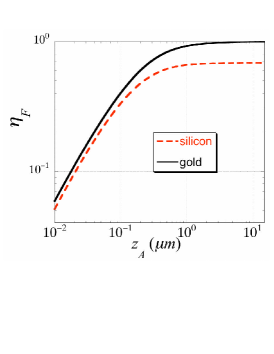
Figure 4: (color online) Correction $\eta_{F}=F^{(0)}/F^{(0)}_{\rm CP}$ of the normal dispersive force between a Rb ground state atom and a plane gold (dark green) or silicon (red) surface as a function of the separation distance $z_{A}$.

V Experimental prospects

There are several possible experimental scenarios where non-trivial geometrical effects of atom-surface forces could be probed. In particular, Bose-Einstein condensates represent an ideal sensor of quantum vacuum forces since they are well controlled and characterized. One possible experiment is to use a BEC as a sensitive oscillator, whose center-of-mass frequency is modified when the BEC is close to a surface Antezza05 . This idea was recently used to measure the normal component of the Casimir-Polder force between a Rb condensate oscillating along the perpendicular direction to a planar dielectric surface Cornell07 . Lateral Casimir-Polder forces could be measured in a similar fashion with an elongated BEC oscillating parallel to the surface, with it long axis parallel to the corrugation axis of a uni-axial corrugated surface JPA ; PRL . We have shown in these references that non-trivial geometrical quantum vacuum effects, beyond the usual proximity force and pair-wise summation approximations, could be measured using present-day cold atom technology. We shall not further discuss this proposal here.

Rather, let us comment briefly on another possible scenario, that although is less sensitive, has the nice feature of measuring directly the atom-surface interaction potential instead of its second derivative, as in the BEC oscillator. The idea is to use a quasi one-dimensional BEC to locally probe potential variations via imaging the local one-dimensional density. Small electric and magnetic fields of BECs in atom chips have been recently probed using this technique Schmiedmayer . Lateral Casimir-Polder forces could be measured with a cigar-shaped BEC placed parallel to the surface and with its long axis perpendicular to the uni-axial corrugation lines. The potential along the quasi one-dimensional BEC is related to the one-dimensional particle density $n_{1d}(x)$ as

$$V_{\rm ho}(x)+V_{\rm CP}(x)=-\hbar\omega_{\rm tr}\sqrt{1+4a_{\rm scat}n_{1d}(x)},$$ (32)

where $V_{\rm ho}(x)$ is the external harmonic trapping potential, $V_{\rm CP}(x)$ is the Casimir-Polder potential, $\omega_{\rm tr}$ is the transverse (strong) trapping frequency, and $a_{\rm scat}$ is the s-wave scattering length. In Schmiedmayer the optimal potential single shot sensitivity $\Delta V$ is estimated as $\Delta V=\gamma\Delta N/\rho_{0}^{2}x_{0}$, where $\gamma=2\hbar^{2}a_{\rm scat}/m$. Here $m$ is the mass of Rb atoms, $\Delta N$ is the detection imaging noise, $x_{0}$ is the longitudinal spatial resolution, and $\rho_{0}$ is the transverse spatial resolution. In the experiment Schmiedmayer , $\omega_{\rm tr}=2\pi\times 300$Hz, $\Delta N\approx 4$ atoms per pixel in a CCD camera, leading to a single-shot single-point sensitivity to potential variations of $\Delta V\approx 10^{-13}-10^{-14}$eV.

For the sake of estimating the order of magnitude of the lateral Casimir-Polder force let us consider a uni-axial corrugated perfectly reflecting surface. We now use our perturbative expansion of the potential in powers of the corrugation profile. In the retarded regime ($z_{A}\gg\lambda_{A}$), the zeroth-order potential is $U^{(0)}(z_{A})=-3\hbar c\alpha(0)/32\pi^{2}\epsilon_{0}z_{A}^{4}$, where $\alpha(0)/4\pi\epsilon_{0}=47.3\times 10^{-30}{\rm m}^{3}$ for ⁸⁷Rb atoms. For a corrugation amplitude $h=100$nm, wavelength $\lambda=10\mu$m and an atom-plate distance $z_{A}=2\mu$m, the correction is $U^{(1)}=1.13\times 10^{-14}$eV, which is on the border of the experimental sensitivity reported in Schmiedmayer . The experimental signal of the lateral Casimir-Polder force would consist on a density modulation of 1d BEC density following the law $n_{\rm 1d}(x)\simeq[V_{\rm ho}(x)+V_{\rm CP}(x)]^{2}$.

Other possible experiments to probe lateral Casimir-Polder forces could involve spin echo techniques for atomic beams flying above corrugated surfaces DeKieviet2003 , or a two-component, phase-separated BEC ”level” Timmermans2008 used as a cold-atom analog of an AFM to map the corrugated surface potential.

VI Conclusions

We have developed a scattering approach to the dispersive force between a ground state atom and a material body. We have focused on the case of a corrugated surface, and derived explicit results to first order in the corrugation amplitude. Exact numerical calculation of the dispersive first-order potential has been represented in terms of the response function $g(k,z_{A}),$ calculated for arbitrary values of the separation distance $z_{A}$ and corrugation wavelength $\lambda=2\pi/k,$ as long as the corrugation amplitude remains much smaller than both length scales. Different atomic species and materials can be considered within our formalism. Here we have illustrated our method by taking Rb atoms on top of gold or silicon surfaces.

For separation distances larger than $1\,\mu{\rm m},$ the response function $g(k,z)$ can be easily obtained from the very simple CP result (30) for the beyond-PFA geometry correction factor $\rho$, together with the numerical values for the real material reduction factor $\eta_{F}$ calculated for the plane geometry.

The position dependence of the resulting potential leads to a lateral dispersive force. We have discussed a variety of possible experiments with Bose-Einstein condensates that would allow for the verification of non-trivial beyond-PFA effects with current state-of-the-art techniques.

Appendix A Scattering matrix for an atomic magnetic dipole moment

Eq. (7) gives the expression of the atomic reflection matrix elements under the assumption that the atom is characterized by an electrical polarizability $\alpha(\omega)$. The expression of the matrix elements of the operator $\mathcal{R}_{A}$ was found starting from the linear relation (4) between the induced atomic electric dipole and the external (incoming) electric field calculated in the position $\mathbf{R}_{A}$ and writing down the electric field produced by the induce dipole moment $\mathbf{d}(\omega)$. In particular, we were interested in the field going towards the surface $(\downarrow)$ as a function of the field coming from it $(\uparrow)$.

A completely analogous calculation can be performed assuming that the fluctuating magnetic field $\mathbf{H}$ induces a magnetic dipole moment $\mathbf{m}$ on the atom given by

$${\bf m}(\omega)=\beta(\omega){\bf H}({\bf R}_{A},\omega),$$ (33)

where $\beta(\omega)$ is the magnetic polarizability. For the field generated by the magnetic dipole in the region $z<z_{A}$ we find the Fourier component

$${E}^{\downarrow}_{({\rm mdip})p}({\bf k},\omega) = -\frac{i\omega}{2\epsilon_{0}c^{2}k_{z}}e^{-i\mathbf{k}\cdot\mathbf{r}_{A}}e^{ik_{z}z_{A}}$$ (34)

$$\times\mbox{\boldmath${\hat{\epsilon}}$}^{-}_{p}(\mathbf{k})\cdot\bigl{(}\mathbf{K}^{-}\times{\bf m}(\omega)\bigr{)}.$$

Using the following expression for the magnetic field coming upwards from the surface

$${\bf H}^{\uparrow}(\mathbf{k},z,\omega)=\frac{1}{\mu_{0}\omega}\sum_{p}{E}_{p}^{\uparrow}({\bf k},\omega)\bigl{(}\mathbf{K}^{+}\times\mbox{\boldmath${\hat{\epsilon}}$}^{+}_{p}({\bf k},\omega)\bigr{)}e^{ik_{z}z},$$ (35)

and replacing Eq. (33) into expression (34) we find

$$\langle\mathbf{k},p|{\cal R}^{m}_{A}|\mathbf{k}^{\prime},p^{\prime}\rangle=-\frac{\beta(i\xi)}{2\kappa}e^{-i(\mathbf{k}-\mathbf{k}^{\prime})\cdot\mathbf{r}_{A}}e^{-(\kappa+\kappa^{\prime})z_{A}}$$

$$\times\hat{\mbox{\boldmath$\epsilon$}}_{p}^{-}(\mathbf{k},i\xi)\cdot\Bigl{[}\mathbf{K}^{-}\times\Bigl{(}\mathbf{K}^{\prime+}\times\hat{\mbox{\boldmath$\epsilon$}}_{p^{\prime}}^{+}(\mathbf{k}^{\prime},i\xi)\Bigr{)}\Bigr{]}.$$ (36)

As a consequence, if we want to include both contributions (electric and magnetic dipole moments), the atomic reflection operator is simply given by the sum of the operators $\mathcal{R}_{A}$ and $\mathcal{R}^{M}_{A}$, given by (7) and (36) respectively. It is possible to check, for example, that for two atoms the scattering formula (II) gives back the known result for the interatomic potential energy in the Casimir-Polder regime Feinberg .

Appendix B Casimir-Polder regime

Simple closed forms for the first-order response function can be derived in some limiting cases. In fact, $g(k,z_{A})$ is given by the integral over the positive imaginary frequency axis of a function involving three quantities that decay to zero: the atomic polarizability $\alpha(i\xi)$, the round-trip propagation factor $\exp[-(\kappa^{\prime}+\kappa^{\prime\prime})z_{A}]$ and the reflection amplitudes $r^{p}(k,i\xi)$ (due to the frequency dependence of the permittivity function). These functions decay on different frequency scales: $c/\lambda_{A}$, $c/z_{A}$ and $\omega_{P}$ (a typical frequency associated to the surface optical response, for example the plasma frequency for metallic media), respectively. As a consequence, the significant range of frequencies giving the main contribution to the integral in (III) will be determined by the smallest of these frequency scales. One can then expect that the integral (III) can be considerably simplified for some particular relations between these frequency scales.

In this Appendix, we consider the case $z_{A}\gg\lambda_{P},\lambda_{A}$, usually referred to as Casimir-Polder regime (note that we assume $z_{A}\ll\hbar c/(k_{B}T)$ so as to neglect thermal corrections). Since the smallest frequency scale is $c/z_{A},$ we can replace the dynamical polarizability $\alpha(i\xi)$ and the permittivity $\epsilon(i\xi)$ by their zero frequency values. For the metallic case, we can take $\epsilon(0)\rightarrow\infty$ and then derive remarkably simple expressions from (24):

$$a_{{\bf k}^{\prime},{\bf k}^{\prime\prime}}=\frac{1}{2}e^{-(\kappa^{\prime}+\kappa^{\prime\prime})z_{A}}$$ (37)

$$\times\left\{\frac{1}{\kappa^{\prime}\kappa^{\prime\prime}}[k^{2}+(\kappa^{\prime}-\kappa^{\prime\prime})^{2}]+\frac{c^{2}}{\xi^{2}}[k^{2}-(\kappa^{\prime}+\kappa^{\prime\prime})^{2}]\right\}.$$

This expression could also have been obtained by taking the usual perfectly-reflecting boundary conditions on the corrugated surface.

After replacing (37) into

$$g_{\rm CP}(k,z_{A})=\frac{\hbar\alpha(0)}{\epsilon_{0}c^{2}}\int_{0}^{\infty}\frac{d\xi}{2\pi}\xi^{2}\int\frac{d^{2}{\bf k}^{\prime}}{(2\pi)^{2}}a_{{\bf k}^{\prime},{\bf k}^{\prime\prime}}(z_{A},\xi),$$

we change the integration variables from $(\xi,k^{\prime},\phi^{\prime})$ to $(\kappa^{\prime},\kappa^{\prime\prime},\varphi)$, taking $k^{\prime}(\kappa^{\prime},\kappa^{\prime\prime},\varphi)=[(\kappa^{\prime})^{2}-(\kappa^{\prime\prime})^{2}+k^{2}]/(2k\cos\phi^{\prime})$ and $\xi(\kappa^{\prime},\kappa^{\prime\prime},\phi^{\prime})=c[(\kappa^{\prime})^{2}-(k^{\prime})^{2}(\kappa^{\prime},\kappa^{\prime\prime},\phi^{\prime})]^{1/2}$. The Jacobian of the transformation is $|J|=2c\kappa^{\prime}\kappa^{\prime\prime}/\{4k^{2}(\kappa^{\prime})^{2}\cos^{2}\phi^{\prime}-[(\kappa^{\prime})^{2}-(\kappa^{\prime\prime})^{2}+k^{2}]\}^{1/2}$. We first use the property $\int_{0}^{2\pi}d\phi^{\prime}(...)=2\int_{0}^{\pi}d\phi^{\prime}(...)$. Then we write the integral as a sum of two contributions:

$$\int_{0}^{\infty}d\kappa^{\prime}\int_{|\kappa^{\prime}-k|}^{\sqrt{(\kappa^{\prime})^{2}+k^{2}}}d\kappa^{\prime\prime}\int_{0}^{\phi_{m}}d\phi^{\prime}$$

and

$$\int_{0}^{\infty}d\kappa^{\prime}\int_{\sqrt{(\kappa^{\prime})^{2}+k^{2}}}^{\kappa^{\prime}+k}d\kappa^{\prime\prime}\int_{\pi-\phi_{m}}^{\pi}d\phi^{\prime},$$

with $\cos\varphi_{m}=[(\kappa^{\prime})^{2}-(\kappa^{\prime\prime})^{2}+k^{2}]/2\kappa^{\prime}k,$ and introduce further auxiliary integration variables $u=\kappa^{\prime}+\kappa^{\prime\prime}$ and $v=\kappa^{\prime}-\kappa^{\prime\prime}$ to obtain the final analytical result

$$g_{\rm CP}^{\rm perf}(k,z_{A})=F_{\rm CP}^{(0)}(z_{A})e^{-\mathcal{Z}}\left(1+\mathcal{Z}+\frac{16\mathcal{Z}^{2}}{45}+\frac{\mathcal{Z}^{3}}{45}\right)$$

$$\mathcal{Z}\equiv kz_{A}$$ (38)

Appendix C Van der Waals regime

In this appendix, we assume that $z_{A}\ll\lambda_{A}$. In this van der Waals regime, one can neglect retardation effects and assume an instantaneous atom-surface interaction (limit $c\to\infty$).

In order to extract some simple expressions for the vdW response function, we have first to choose a specific expression for the atomic polarizability $\alpha(i\xi)$. We will use the following model function suitable for a multilevel isotropic atom having transition frequencies $\omega_{n0}$ from the $n$-th excited state to the ground state and electric dipole matrix elements $d_{n0}$ on these transitions

$$\alpha(i\xi)=\frac{2}{3\hbar}\sum_{n}\frac{\omega_{n0}d_{n0}^{2}}{\omega_{n0}^{2}+\xi^{2}},$$ (39)

Then we have to specify the transmission and reflection amplitude functions. Here we take Fresnel formulas with two different models for the permittivity $\epsilon(i\xi)$.

Plasma metals. We first take the plasma model for metallic materials:

$$\epsilon(i\xi)=1+\frac{\omega_{P}^{2}}{\xi^{2}}.$$ (40)

In this case we obtain from (III)-(24)

$$g_{\rm vdW}(k,z_{A})=-\sum_{n}\frac{kd_{n0}^{2}x_{n}}{192\sqrt{2}\pi\epsilon_{0}z_{A}^{3}(x_{n}^{2}+2\sqrt{2}x_{n}+2)}\Bigl{[}6\sqrt{2}{\cal Z}(x_{n}+\sqrt{2})K_{0}({\cal Z})+(\sqrt{2}({\cal Z}^{2}+12)x_{n}+{\cal Z}^{2}+24)K_{1}({\cal Z})\Bigr{]},$$ (41)

where $x_{n}=\omega_{P}/\omega_{n0}$ and ${\cal Z}=kz_{A}$. If we let all the $x_{n}$ go to infinity, we get the result for a perfect conductor PRL

$$g^{\rm perf}_{\rm vdW}(k,z_{A}) = -\sum_{n}\frac{kd_{n0}^{2}}{192\pi\epsilon_{0}z_{A}^{3}}$$

$$\times\Bigl{[}6{\cal Z}K_{0}({\cal Z})+({\cal Z}^{2}+12)K_{1}({\cal Z})\Bigr{]}.$$

In the opposite limit, with $\omega_{P}\ll\omega_{n0}$ for all $n,$ we derive from (41) the plasmon van der Waals limit

$$g_{\rm vdW}^{\rm plas}(k,z_{A}) = -\sum_{n}\frac{kd_{n0}^{2}x_{n}}{384\sqrt{2}\pi\epsilon_{0}z_{A}^{3}}$$

$$\times\Bigl{[}12{\cal Z}K_{0}({\cal Z})+({\cal Z}^{2}+24)K_{1}({\cal Z})\Bigr{]}.$$

This result is, as expected, proportional to the plasma frequency $\omega_{P}$.

Semiconductors: In order to treat the case of semiconductors, we assume that the material can be described by the Drude-Lorentz model function

$$\epsilon(i\xi)=1+\frac{\omega_{DL}^{2}(\epsilon(0)-1)}{\omega_{DL}^{2}+\xi^{2}}.$$ (44)

In this case we get

$$\begin{split}g_{\rm vdW}(k,z_{A})&=-\sum_{n}\frac{\gamma kd_{n0}^{2}x_{n}}{384\pi\epsilon_{0}z_{A}^{3}(\gamma+2)^{\frac{3}{2}}((\gamma+2)x_{n}^{2}-2)^{2}}\Bigl{(}12A_{0}{\cal Z}K_{0}({\cal Z})+A_{1}({\cal Z})K_{1}({\cal Z})\Bigr{)}\\ A_{0}&=(\gamma+2)(\sqrt{\gamma+2}x_{n}-\sqrt{2})((\gamma+2)x_{n}^{2}-2)\\ A_{1}&=2(\gamma+2)^{\frac{3}{2}}(({\cal Z}^{2}+12)\gamma+24)x_{n}^{3}-3\sqrt{2}(\gamma+2)(({\cal Z}^{2}+8)\gamma+16)x_{n}^{2}-48(\gamma+2)^{\frac{3}{2}}x_{n}+2\sqrt{2}(({\cal Z}^{2}+24)\gamma+48)\\ \end{split}$$ (45)

where $\gamma=\epsilon(0)-1$ and $x_{n}=\omega_{DL}/\omega_{n0}$.

References

- (1) C.I. Sukenik, M.G. Boshier, D. Cho, V. Sandoghdar, and E.A. Hinds, Phys. Rev. Lett. 70, 560 (1993).
- (2) A. Landragin, J.Y. Courtois, G. Labeyrie, N. Vansteenkiste, C.I. Westbrook, and A. Aspect, Phys. Rev. Lett. 77, 1464 (1996).
- (3) F. Shimizu, Phys. Rev. Lett. 86, 987 (2001).
- (4) V. Druzhinina and M. DeKieviet, Phys. Rev. Lett. 91, 193202 (2003).
- (5) T.A. Pasquini, Y. Shin, C. Sanner, M. Saba, A. Shirotzek, D.E. Pritchard, and W. Ketterle, Phys. Rev. Lett. 93, 223201 (2004); T.A. Pasquini, M. Saba, G.B. Jo, Y. Shin, W. Ketterle, D.E. Pritchard, T.A. Sabas, and N. Mulders, Phys. Rev. Lett. 97, 093201 (2006).
- (6) D.M. Harber, J.M. Obrecht, J.M. McGuirk, and E.A. Cornell, Phys. Rev. A 72, 033610 (2005).
- (7) J.M. Obrecht, R.J. Wild, M. Antezza, L.P. Pitaevskii, S. Stringari, and E.A. Cornell, Phys. Rev. Lett. 98, 063201 (2007).
- (8) Y.J. Lin, I. Teper, C. Chin, and V. Vuletic, Phys. Rev. Lett. 92, 050404 (2004).
- (9) Conference on atoms and molecules near surfaces (CAMS), J. Phys.: Conf. Ser. 19 (2005).
- (10) H.B.G. Casimir and D. Polder, Phys. Rev. 73, 360 (1948).
- (11) F.S.S. Rosa, D.A.R. Dalvit, and P.W. Milonni, Phys. Rev. A 78, 032117 (2008).
- (12) L.P. Pitaevskii, Phys. Rev. Lett. 101, 163202 (2008).
- (13) S.Y. Buhmann and D.-G. Welsch, Prog. Quantum Electron. 31, 51 (2007), and references therein.
- (14) M. Antezza, L.P. Pitaevskii, and S. Stringari, Phys. Rev. Lett. 95, 113202 (2005).
- (15) V. Druzhinina, M. Mudrich, F. Arnecke, J. Madroñero, and A. Buchleitner, arXiv:0810.4281.
- (16) B.V. Derjaguin and I.I. Abrikosova, Sov. Phys. JETP 3, 819 (1957); B.V. Derjaguin, Sci. Am. 203, 47 (1960).
- (17) See, for instance, V.B. Bezerra, G.L. Klimchitskaya, and C. Romero, Phys. Rev. A 61, 022115 (2000).
- (18) D.A.R. Dalvit, P.A. Maia Neto, A. Lambrecht, and S. Reynaud, J. Phys. A: Math. Theor. 41, 164028 (2008).
- (19) D.A.R. Dalvit, P.A. Maia Neto, A. Lambrecht, and S. Reynaud, Phys. Rev. Lett. 100, 040405 (2008).
- (20) H.B. Chan, Y. Bao, J. Zou, R.A. Cirelli, F. Klemens, W.M. Mansfield, and C.S. Pai, Phys. Rev. Lett. 101, 030401 (2008). The exact solution for the Casimir force in this configuration has been recently found using the scattering approach in Lambrecht08 .
- (21) A. Lambrecht and V. N. Marachevsky, Phys. Rev. Lett. 101, 1160403 (2008).
- (22) M. Babiker and G. Barton, J. Phys. A (London) 9, 129 (1979).
- (23) J. M. Wylie and J. E. Sipe, Phys. Rev. A 30, 1185 (1984).
- (24) J. F. Babb, G. L. Klimchitskaya and V. M. Mostepanenko Phys. Rev. A 70, 042901 (2004).
- (25) S.Y. Buhman, D.-G. Welsch and T. Kampf, Phys. Rev. A 72, 032112 (2005).
- (26) B. Döbrich, M. DeKieviet, and H. Gies, arXiv:0810.3480.
- (27) E. M. Lifshitz, Sov. Phys. JETP 2, 73 (1956).
- (28) I.E. Dzyaloshinskii and L.P. Pitaevskii, Sov. Phys. JETP 9, 1282 (1959); I.E. Dzyaloshinskii, E.M. Lifshitz, and L.P. Pitaevskii, Adv. Phys. 10, 165 (1961).
- (29) E.I. Kats, JETP 46, 109 (1977).
- (30) A. Lambrecht, P.A. Maia Neto and S. Reynaud, New J. Phys. 8, 243 (2006).
- (31) M.T. Jaekel and S. Reynaud, J. Physique I-1, 1395 (1991) [arXiv:quant-ph/0101067].
- (32) C. Genet, A. Lambrecht and S. Reynaud, Phys. Rev. A 67, 043811 (2003).
- (33) P.A. Maia Neto, A. Lambrecht, and S. Reynaud, Europhys. Lett. 69, 924 (2005); Phys. Rev. A 72, 012115 (2005). The second paper contains a typo in Eq. (36), since the matrix is expressed as . The correct formula, with and exchanged, is the expression given in the present paper.
- (34) R.B. Rodrigues, P.A. Maia Neto, A. Lambrecht and S. Reynaud, Phys. Rev. Lett. 96, 100402 (2006); Phys. Rev. A 75, 062108 (2007).
- (35) A. Bulgac, P. Magierski and A. Wirzba, Phys. Rev. D 73, 025007 (2006).
- (36) M. Bordag, Phys. Rev. D 73, 125018 (2006).
- (37) T. Emig, J. Stat. Mech.: Theory Exp. 2008, P04007.
- (38) P.A. Maia Neto, A. Lambrecht and S. Reynaud, Phys. Rev. A 78, 012115 (2008).
- (39) T. Emig, N. Graham, R.L. Jaffe and M. Kardar, Phys. Rev. Lett 99, 170403 (2007).
- (40) O. Kenneth and I. Klich, Phys. Rev. B 78, 014103 (2008).
- (41) Dimensionally speaking, is equal to times a volume. The latter volume (i.e. ) is identified with the polarizability in the “electrostatic cgs” unit system, used in a number of papers studying dispersion forces. This point has to be treated carefully when comparing various expressions.
- (42) R. Carminati, M. Nieto-Vesperinas and J.-J. Greffet, J. Opt. Soc. Am. A 15, 706 (1998).
- (43) For consistency, higher-order multipoles beyond the electric dipole approximation for the atom-field coupling would also be needed to compute corrections involving higher powers of .
- (44) G. Feinberg and J. Sucher, Phys. Rev. A 2, 2395 (1970).
- (45) M. Antezza, L. P. Pitaevskii and S. Stringari, Phys. Rev. A 70, 053619 (2004).
- (46) J.-J. Greffet, Phys. Rev. B 37, 6436 (1988).
- (47) G. S. Agarwal, Phys. Rev. B 15, 2371 (1977).
- (48) A. Derevianko, W.R. Johnson, M.S. Safronova, and J.F. Babb, Phys. Rev. Lett. 82, 3589 (1999).
- (49) Handbook of Optical Constants of Solids, edited by E. Palik (Academic Press, New York, 1998).
- (50) A. Lambrecht and S. Reynaud, Eur. Phys. J. D 8, 309 (2000).
- (51) I. Pirozhenko and A. Lambrecht, Europhys. Lett. 77, 44006 (2007).
- (52) Handbook of Mathematical Functions, edited by M. Abramowitz and I. Stegun (Dover, New York, 1972).
- (53) S. Wildermuth, S. Hofferberth, I. Lesanovsky, E. Haller, L.M. Anderson, S. Groth, I. Ber-Joseph, P. Krüger, and J. Schmiedmayer, Nature 435, 440 (2005); P. Krüger, S. Wildermuth, S. Hofferberth, L.M. Anderson, S. Groth, I. Bar-Joseph, and J. Schmiedmayer, J. Phys.: Conference Series 19, 56 (2005); S. Wildermuth, S. Hofferberth, I. Lesanovsky, S. Groth, P. Krüger, J. Schmiedmayer, and I. Bar-Joseph, Applied Phys. Lett. 88, 264103 (2006).
- (54) S.G. Bhongale and E. Timmermans, Phys. Rev. Lett. 100, 185301 (2008).