Theoretical expectations for a fractional quantum Hall effect in graphene

Abstract

Due to its fourfold spin-valley degeneracy, graphene in a strong magnetic field may be viewed as a four-component quantum Hall system. We investigate the consequences of this particular structure on a possible, yet unobserved, fractional quantum Hall effect in graphene within a trial-wavefunction approach and exact-diagonalisation calculations. This trial-wavefunction approach generalises an original idea by Halperin to account for the SU(2) spin in semiconductor heterostructures with a relatively weak Zeeman effect. Whereas the four-component structure at a filling factor $\nu=1/3$ adds simply a SU(4)-ferromagnetic spinor ordering to the otherwise unaltered Laughlin state, the system favours a valley-unpolarised state at $\nu=2/5$ and a completely unpolarised state at $\nu=4/9$. Due to the similar behaviour of the interaction potential in the zero-energy graphene Landau level and the first excited one, we expect these states to be present in both levels.

1 Introduction

Electrons in graphene may be viewed as a particular form of the two-dimensional electron gas (2DEG), with the fundamental difference that, due to the particular band structure, their low-energy properties are discribed in terms of a zero-mass Dirac equation rather than the usual effective-mass Schrödinger equation [1]. One of the most salient features of the 2DEG, when submitted to a strong magnetic field, is the quantum Hall effect which occurs in an integer (IQHE) as well as in a fractional (FQHE) form. The former is also manifest in graphene [2, 3], and its obervation is a spectacular proof of relativistic electrons (and holes) in graphene, due to an unusual quantisation of the Hall conductivity, $\sigma_{H}=2(e^{2}/h)(2n+1)$, in terms of the integer $n$, as expected on theoretical grounds [4, 5, 6].

Experimental evidence for the FQHE, which is due to electron-electron interactions in a partially filled Landau level (LL), is yet lacking in graphene. In the usual 2DEG in GaAs/AlGaAs heterostructures, the FQHE is, indeed, seen in samples with high mobilities yet unaccessed in graphene on a SiO₂ substrate ($\mu\sim 50\,000\,{\rm cm^{2}/Vs}$ for typical samples). Higher mobilities ($\mu\sim 200\,000\,{\rm cm^{2}/Vs}$) have been achieved in current-annealed suspended graphene [7], but unexpectedly the IQHE happens to break down above 1T, probably due to extrinsic effects that are not related to the intrinsic electronic properties of these graphene samples [8]. In spite of the missing FQHE, interaction physics is likely to be at the origin of additional plateaus in the Hall conductivity at LL filling factors $\nu_{G}=\pm 1$ (and 0) [9], where $\nu_{G}=n_{C}/n_{B}$ is the ratio between the carrier density ($n_{C}>0$ for electron and $n_{C}<0$ for hole transport) and that, $n_{B}=B/(h/e)$ of the flux quanta threading the graphene sheet.

From a theoretical point of view, interactions in graphene LLs are expected to be relevant. Indeed, one needs to compare the typical energy for exchange interaction $V_{C}=e^{2}/\epsilon R_{C}\simeq 25\sqrt{B[{\rm T}]}/\epsilon\sqrt{2n+1}$ meV, in terms of the dielectric constant $\epsilon$ and the cyclotron radius $R_{C}=l_{B}\sqrt{2n+1}$, with the magnetic length $l_{B}=\sqrt{\hbar/eB}=25/\sqrt{B[{\rm T}]}\,{\rm nm}$, to the LL separation $\Delta_{n}=\sqrt{2}\hbar(v_{F}/l_{B})(\sqrt{n+1}-\sqrt{n})$, where $v_{F}$ is the Fermi velocity. In spite of the decreasing LL separation in the large-$n$ limit, the ratio between both energy scales remains constant and reproduces the fine-structure constant of graphene, $\alpha_{G}=V_{C}/\Delta_{n}=e^{2}/\hbar v_{F}\epsilon\simeq 2.2/\epsilon$. Notice that the Coulomb interaction respects the fourfold spin-valley degeneracy to lowest order in $a/l_{B}\simeq 0.005\sqrt{B[{\rm T}]}$, where $a=0.14$ nm is the distance between nearest-neighbour carbon atoms in graphene. This fourfold spin-valley symmetry is described in the framework of the SU($4$) group which covers the two copies of the SU(2) spin and the SU(2) valley isospin. Lattice effects break this SU(4) symmetry at an energy scale $V_{C}(a/l_{B})\simeq 0.1B[{\rm T}]/\epsilon$ meV [10, 11, 12, 13], which is roughly on the same order of magnitude as the expected Zeeman effect in graphene [9]. Other symmetry-breaking mechanisms have been proposed [14, 15, 16] but happen to be equally suppressed with respect to the leading interaction energy scale $V_{C}$. An exception may be graphene on a graphite substrate, where the natural lattice commensurability of the substrate and the sample may lead to a stronger coupling than for graphene on a SiO₂ substrate [17]. This yields a mass term in the Dirac Hamiltonian which lifts the valley degeneracy of the zero-energy LL [14].

Based on these considerations, graphene in a strong magnetic field may thus be viewed as a four-component quantum Hall system, and we neglect SU(4)-symmetry breaking terms in the remainder of the paper. An interesting theoretical expectation resulting from this feature is the formation of a quantum Hall ferromagnet at $\nu=\pm 1$ [18, 10, 11, 19] with SU(4)-skyrmion excitations, which may have peculiar magnetic properties [19, 20]. Also for the FQHE, the SU(4) spin-valley symmetry is expected to play a relevant role and has been considered within a composite-fermion approach [21] as well as one based on SU(4) Halperin wavefunctions [22, 23].

In this paper, we review how the four-component structure of graphene may have particular signatures in a possible FQHE. In a first step, we discuss the structure of the interaction model for electrons restricted to a single graphene LL. We concentrate on the spin-valley SU(4) symmetric part of the interaction model, which constitutes the leading energy scale, and discuss, based on the behaviour of the pseudopotentials, theoretical expectations for the FQHE in graphene in the LLs $n=0$ and $1$. In the second part of this paper, we corroborate these qualitative expectations with the help of the SU(4) wavefunction approach [22, 23] and exact-diagonalisation calculations.

2 Interaction model

In the case of a partially filled LL, one may separate the “low-energy” degrees of freedom, which consist of intra-LL excitations, from the “high-energy” inter-LL excitations. In the absence of disorder, all states within the partially filled LL have the same kinetic energy such that intra-LL excitations may be described by considering only electron-electron interactions,

$$H_{\lambda n}=\frac{1}{2}\sum_{{\bf q}}v(q)\rho_{\lambda n}(-{\bf q})\rho_{\lambda n}({\bf q}),$$ (1)

where $v(q)=2\pi e^{2}/\epsilon q$ is the 2D Fourier-transformed Coulomb interaction potential. The Fourier components $\rho_{\lambda n}({\bf q})$ of the density operator are constructed solely from states within the $n$-th LL in the band $\lambda$ ($\lambda=+$ for the conduction and $\lambda=-$ for the valence band). This construction is analogous to that used in the conventional 2DEG, but the density operators $\rho_{n}({\bf q})$ are now built up from spinor states of the 2D Dirac equation,

$$\psi_{\lambda n,m}^{\xi}=\frac{1}{\sqrt{2}}\left(\begin{array}[]{c}|n-1,m\rangle\\ \lambda|n,m\rangle\end{array}\right)$$ (2)

for $n\neq 0$ and

$$\psi_{n=0,m}^{\xi}=\left(\begin{array}[]{c}0\\ |n=0,m\rangle\end{array}\right)$$ (3)

for the zero-energy LL $n=0$, in terms of the harmonic oscillator states $|n,m\rangle$ and the guiding-centre quantum number $m=0$. Here, we have chosen the first component of the spinor to represent at the $K$ point ($\xi=+$) the amplitude on the $A$ sublattice and that on the $B$ sublattice at the $K^{\prime}$ point ($\xi=-$). Notice that the valley and the sublattice indices happen to be the same in the zero-energy LL $n=0$ and that, thus, a perturbation that breaks the inversion symmetry (the equivalence of the two sublattices) automatically lifts the valley degeneracy [14, 15, 16]. In terms of the spinor states (2) and (3), the density operator may be written

$$\rho_{\lambda n}({\bf q})=\sum_{\xi,m}\left(\psi_{\lambda n,m}^{\xi}\right)^{\dagger}e^{-i{\bf q}\cdot{\bf r}}\psi_{\lambda n,m^{\prime}}^{\xi}c_{\lambda n,m;\xi}^{\dagger}c_{\lambda n,m^{\prime};\xi}\ ,$$ (4)

where $c_{\lambda n,m;\xi}^{(\dagger)}$ annihilates (creates) an electron in the state $\psi_{\lambda n,m}^{\xi}$. In Eq. (4), we have neglected the contributions that are off-diagonal in the valley index. Indeed, these contributions give rise to a rapidly oscillating phase $\exp(\pm i{\bf K}\cdot{\bf r})$ in the matrix elements, where $\pm{\bf K}=\pm(4\pi/3\sqrt{3}a){\bf e}_{x}$ is the location of the $K$ and $K^{\prime}$ points, respectively, and yield terms in the Hamiltonian (1), which break the valley-SU(2) symmetry of the interaction. They are suppressed by a factor $a/l_{B}$ with respect to the leading interaction energy scale $e^{2}/\epsilon l_{B}$ [10], as mentioned in the introduction. For the sake of simplicity and because of their smallness, we neglect these terms here.

Within the symmetric gauge, ${\bf A}=(B/2)(-y,x,0)$, the position operator ${\bf r}$ in Eq. (4) may be decomposed into the guiding-centre position ${\bf R}$ and the cyclotron variable $\eta$. Whereas the latter only affects the quantum number $n$, ${\bf R}$ acts on $m$, and we may therefore rewrite the density operator (4), $\rho_{\lambda n}({\bf q})=\mathcal{F}_{n}({\bf q})\bar{\rho}({\bf q})$, as a product of the projected density operator

$$\bar{\rho}({\bf q})=\sum_{\xi;m,m^{\prime}}\left\langle m\left|e^{-i{\bf q}\cdot{\bf R}}\right|m^{\prime}\right\rangle c_{\lambda n,m;\xi}^{\dagger}c_{\lambda n,m^{\prime};\xi}$$ (5)

and the graphene form factor

$$\mathcal{F}_{n}(q) = \frac{1}{2}\left(\left\langle n-1\left|e^{-i{\bf q}\cdot\mbox{\boldmath$\eta$}}\right|n-1\right\rangle+\left\langle n\left|e^{-i{\bf q}\cdot\mbox{\boldmath$\eta$}}\right|n\right\rangle\right)$$

$$= \frac{1}{2}\left[L_{n-1}\left(\frac{q^{2}l_{B}^{2}}{2}\right)+L_{n}\left(\frac{q^{2}l_{B}^{2}}{2}\right)\right]e^{-q^{2}l_{B}^{2}/4}$$

for $n\neq 0$, in terms of Laguerre polynomials, and

$$\mathcal{F}_{n=0}(q)=\left\langle 0\left|e^{-i{\bf q}\cdot\mbox{\boldmath$\eta$}}\right|0\right\rangle=e^{-q^{2}l_{B}^{2}/4}$$ (7)

for $n=0$. With the help of the projected density operators, the interaction Hamiltonian (1) reads

$$H_{\lambda n}=\frac{1}{2}\sum_{{\bf q}}v_{n}^{G}(q)\bar{\rho}(-{\bf q})\bar{\rho}({\bf q}),$$ (8)

where we have defined the effective interaction potential for graphene LLs,

$$v_{n}^{G}(q)=\frac{2\pi e^{2}}{\epsilon q}\left[\mathcal{F}_{n}(q)\right]^{2}.$$ (9)

Notice that the structure of the Hamiltonian (8) is that of electrons in a conventional 2DEG restricted to a single LL if one notices that the projected density operators satisfy the magnetic translation algebra [24]

$$[\bar{\rho}({\bf q}),\bar{\rho}({\bf q}^{\prime})]=2i\sin\left(\frac{{\bf q}^{\prime}\wedge{\bf q}l_{B}^{2}}{2}\right)\bar{\rho}({\bf q}+{\bf q}^{\prime}),$$ (10)

where ${\bf q}^{\prime}\wedge{\bf q}\equiv q_{x}^{\prime}q_{y}-q_{x}q_{y}^{\prime}$ is the 2D vector product. This is a remarkable result in view of the different translation symmetries of the zero-field Hamiltonian; whereas the electrons in the 2DEG are non-relativistic and therefore satisfy Galilean invariance, the relativistic electrons in graphene are Lorentz-invariant. However, once submitted to a strong magnetic field and restricted to a single LL, the translation symmetry of the electrons is described by the magnetic translation group in both cases.

2.1 SU(4) symmetry

The most salient difference between the conventional 2DEG and graphene arises from the larger internal symmetry of the latter, due to its valley degeneracy. This valley degeneracy may be accounted for by an SU(2) valley isospin in addition to the physical SU(2) spin, which we have omitted so far and the symmetry of which is respected by the interaction Hamiltonian. Similarly to the projected charge density operator (5), we may introduce spin and isospin density operators, $\bar{S}^{\mu}({\bf q})$ and $\bar{I}^{\mu}({\bf q})$, respectively, with the help of the tensor products [20]

$$\bar{S}^{\mu}({\bf q}) = \left(S^{\mu}\otimes\mathbbm{1}\right)\otimes\bar{\rho}({\bf q}),$$

$$\bar{I}^{\mu}({\bf q}) = \left(\mathbbm{1}\otimes I^{\mu}\right)\otimes\bar{\rho}({\bf q}).$$ (11)

Here, the operators $S^{\mu}$ and $I^{\mu}$ are (up to a factor $1/2$) Pauli matrices, which act on the spin and valley isospin indices, respectively. The operators $(S^{\mu}\otimes\mathbbm{1})$ and $(\mathbbm{1}\otimes I^{\mu})$ may also be viewed as the generators of the SU(2)$\times$SU(2) symmetry group, which is smaller than the abovementioned SU(4) group. However, once combined in a tensor product with the projected density operators $\bar{\rho}({\bf q})$, the SU(2)$\times$SU(2)-extended magnetic translation group is no longer closed due to the non-commutativity of the Fourier components of the projected density operators. By commutating $[\bar{S}^{\mu}({\bf q}),\bar{I}^{\nu}({\bf q})]$, one obtains the remaining generators of the SU(4)-extended magnetic translation group [20], which is, thus, the relevant symmetry that describes the physical properties of electrons in graphene restricted to a single LL.

2.2 Effective interaction potential and pseudopotentials

Another difference, apart from the abovementioned larger internal symmetry, between the 2DEG and graphene in a strong magnetic field arises from the slightly different effective interaction potentials in the $n$-th LL. The effective interaction for graphene is given by Eq. (9) whereas that in the conventional 2DEG reads

$$v_{n}^{2DEG}(q)=\frac{2\pi e^{2}}{\epsilon q}\left[L_{n}\left(\frac{q^{2}l_{B}^{2}}{2}\right)e^{-q^{2}l_{B}^{2}/4}\right]^{2}.$$ (12)

The difference between the two of them vanishes for $n=0$, as well as in the large-$n$ limit [10], but leads to quite important physical differences in the first excited LL ($n=1$) when comparing graphene to the 2DEG.

For the discussion of the FQHE, it is more appropriate to use Haldane’s pseudopotential construction [25], which is an expansion of the effective interaction potential in the basis of two-particle states with a fixed relative angular momentum $\ell$. In the Laughlin state at filling factor $\nu=1/m$ [26],

$$\phi_{m}^{L}(\{z_{j},z_{j}^{*}\})=\prod_{k<l}(z_{k}-z_{l})^{m}e^{-\sum_{j}|z_{j}|^{2}/4},$$ (13)

in terms of the complex position $z_{j}=(x_{j}+iy_{j})/l_{B}$ of the $j$-th particle, e.g., no particle pair has a relative angular momentum less than $\ell=m$. Therefore, all pseudopotentials $V_{\ell<m}$ are completely screened, and the Laughlin state (13) is the exact $N$-particle ground state with zero energy of a model interaction potential with $V_{\ell<m}>0$ and $V_{\ell\geq m}=0$ [25]. Although this model interaction potential is quite different from the pseudopotentials of the effective interaction potentials (9) and (12), it allows one to generate numerically the Laughlin state, which may be then compared to those obtained within exact-diagonalisation calculations of the realistic interaction potential.

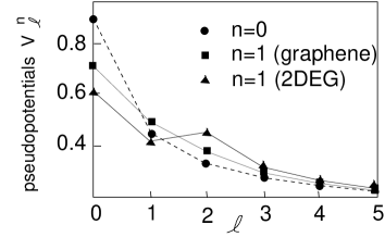
Figure 1: Pseudopotentials for graphene and the 2DEG in $n=0$ (graphene and 2DEG, circles), $n=1$ (graphene, squares), and $n=1$ (2DEG, triangles). The energy is measured in units of $e^{2}/\epsilon l_{B}$. The lines are a guide to the eye.

Notice that one may easily obtain the pseudopotentials of a given interaction potential $v_{n}(q)$ in Fourier space, such as (12) or (9), with the help of

$$V_{\ell}^{n}=\sum_{{\bf q}}v_{n}(q)L_{\ell}(q^{2}l_{B}^{2})e^{-q^{2}l_{B}^{2}/2}.$$ (14)

The pseudopotentials for $n=0$ and $n=1$ in graphene and the 2DEG are shown in Fig. 1, which allows us to make some qualitative statements about a potential FQHE in graphene as compared to that of the 2DEG. First, apart from the internal symmetry, the polarised FQHE states in the zero-energy LL are expected to be the same in graphene as in the 2DEG because there is no difference in the effective interaction potential. The only difference stems from the larger internal symmetry in graphene, which affects the unpolarised FQHE states in $n=0$. Second, the $n=1$ LL in graphene is much more reminiscent of the $n=0$ LL than of the $n=1$ LL in the 2DEG. From an interaction point of view, one would therefore expect that the quantum phases encountered in the $n=1$ graphene LL are merely a copy of those in $n=0$. Furthermore, if one considers spin-polarised FQHE states, only pseudopotentials with odd angular momentum are relevant due to the fermionic nature of the electrons. It is apparent from Fig. 1 that odd-$\ell$ pseudopotentials are systematically larger in $n=1$ than in $n=0$. Therefore, the overall energy scale of FQHE states in $n=1$ is slightly larger (by $\sim 10\%$) than in $n=0$, and one would expect, somewhat counterintuitively, that the $n=1$ FQHE states are more stable than those in $n=0$, for the same $B$-field value. These qualitative predictions [10] have been corroborated within exact-diagonalisation studies, where only the valley isospin degree of freedom was considered and the physical spin was taken as completely polarised [27, 28].

3 Trial wavefunctions

In order to account for the internal SU(4) symmetry in graphene LLs, two of us have proposed a trial-wavefunction approach [22] based on an original idea by Halperin [29] for the description of two-component FQHE states. These states,

$$\psi_{m_{1},...,m_{K};n_{ij}}^{SU(4)}=\phi_{m_{1},...,m_{4}}^{L}\phi_{n_{ij}}^{inter}e^{-\sum_{j=1}^{K}\sum_{k_{j}=1}^{N_{j}}|z_{k_{j}}^{(j)}|^{2}/4},$$ (15)

consist of a product of four Laughlin wavefunctions (13) (one per spin-valley component)

$$\phi_{m_{1},...,m_{K}}^{L}=\prod_{j=1}^{4}\prod_{k_{j}<l_{j}}^{N_{j}}\left(z_{k_{j}}^{(j)}-z_{l_{j}}^{(j)}\right)^{m_{j}}$$

and a term

$$\phi_{n_{ij}}^{inter}=\prod_{i<j}^{4}\prod_{k_{i}}^{N_{i}}\prod_{k_{j}}^{N_{j}}\left(z_{k_{i}}^{(i)}-z_{k_{j}}^{(j)}\right)^{n_{ij}}$$

that takes into account correlations between the different components, labeled by the indices $i,j=1,...,4$. Whereas the exponents $m_{j}$ must be odd integers to account for the fermionic statistics of the electrons, the exponents $n_{ij}$, which describe inter-component correlations, may also be even. Notice further that not all wavefunctions are good candidates for a possible FQHE in graphene; it has indeed been shown, within the plasma analogy [26], that some wavefunctions correspond to a liquid in which the components undergo a spontaneous phase separation [23].

The exponents $n_{ij}$ and $n_{jj}\equiv m_{j}$ define a symmetric $4\times 4$ matrix $M=(n_{ij})$, which determines the component densities $\rho_{j}$ – or else the component filling factors $\nu_{j}=\rho_{j}/n_{B}$,

$$\left(\begin{array}[]{c}\nu_{1}\\ \nu_{2}\\ \nu_{3}\\ \nu_{4}\end{array}\right)=M^{-1}\left(\begin{array}[]{c}1\\ 1\\ 1\\ 1\end{array}\right).$$ (16)

Eq. (16) is only well-defined if the matrix $M$ is invertible. If $M$ is not invertible, some of the component filling factors, e.g. $\nu_{1}$ and $\nu_{2}$, remain unfixed, but not necessarily the sum of the two ($\nu_{1}+\nu_{2}$). This is a particular feature of possible underlying ferromagnetic properties of the wavefunction [22], as is discussed below for some special cases.

In the following, we consider some particular subclasses of the trial wavefunctions (15), which are natural candidates for a FQHE in graphene. Explicitely, we attribute the four spin-valley components as $1=(\uparrow,K)$, $2=(\uparrow,K^{\prime})$, $3=(\downarrow,K)$, and $4=(\downarrow,K^{\prime})$, where the first component denotes the spin orientation ($\uparrow$ or $\downarrow$) and the second the valley ($K$ or $K^{\prime}$). We investigate wavefunctions, where all intracomponent exponents are identical $m_{i}=m$, i.e. we consider the same interaction potential for any of the components, as it is the case in graphene. Furthermore, we consider $n_{13}=n_{24}\equiv n_{a}$ and $n_{12}=n_{14}=n_{23}=n_{34}\equiv n_{e}$, which makes an explicit distinction between inter-component correlations in the same valley ($n_{a}$) and those in different valleys ($n_{e}$). This distinction may occur somewhat arbitrary – indeed, it does no longer treat the spin on the same footing as the valley isospin – but it happens to be useful in some cases if one intends to describe states with intermediate polarisation, such as for a moderate Zeeman field. The equivalence between spin and valley isospin is naturally restored for $n_{e}=n_{a}$. We use the notation $[m;n_{e},n_{a}]$ to describe these subclasses of trial wavefunctions (15), the validity of which we check by exact diagonalisation of $N$ particles on a sphere [25].

3.1 $[m;m,m]$ wavefunctions

If all exponents are identical odd integers $m$, we obtain a completely antisymmetric orbital wavefunction, which is nothing other than the Laughlin wavefunction (13). In this case, the distinction between the components vanishes, and the component filling factors are not fixed – one may, without changing the orbital wavefunction, fill only one particular component as well as another or distribute the particles over all components. Only the total filling factor is fixed at $\nu=1/m$. The corresponding exponent matrix $M$ is indeed not invertible (of rank 1), and the residual freedom of distributing the electrons over the four components may be viewed as the arbitrary orientation of a four-spinor in SU(4) space. The Laughlin wavefunction in graphene is therefore associated with an SU(4) ferromagnetism, similar to that of the state at $\nu_{G}=\pm 1$ [18, 10, 11, 19, 20], where a graphene quantum Hall effect has been observed at high magnetic fields [9].

As already mentioned above, the Laughlin wavefunction has the good property of screening all pseudopotentials with angular momentum $\ell<m$ and has, for $m=3$, the usual large overlap with the Coulomb ground state [21].

3.2 $[m;m-1,m]$ wavefunctions

A similarly good wavefunction is $[m;m-1,m]$, where the intervalley-component exponents are decreased by one. It also screens all pseudopotentials $V_{\ell<m}$ in any pair of electrons within the same valley, but an electron pair in two different valleys is affected by the pseudopotential $V_{\ell=m-1}$. The filling factor, where this wavefunction may occur, is

$$\nu=\frac{2}{2m-1},$$

i.e. at slightly larger densities as the Laughlin wavefunction with the same $m$. The exponent matrix $M$ is still not invertible but of rank 2, and indeed only the filling factors in the two valleys, $\nu_{K}=\nu_{1}+\nu_{3}$ and $\nu_{K^{\prime}}=\nu_{2}+\nu_{4}$, respectively, are fixed, $\nu_{K}=\nu_{K^{\prime}}=1/(2m-1)$. The wavefunction, thus, describes a state with ferromagnetic spin ordering, but which is valley-isospin unpolarised. One may alternatively view this $[m;m-1,m]$ wavefunction as a tensor product of an SU(2) Halperin $(m,m,m-1)$ isospin-singlet wavefunction [29] and a completely symmetric (ferromagnetic) two-spinor that describes the physical spin.

number of particles $N$	4	6	8	10
overlap $\mathcal{O}$ in $n=0$	0.990	0.985	0.979	0.970
overlap $\mathcal{O}$ in $n=1$	0.965	0.882	0.896	0.876

Table 1: Overlap $\mathcal{O}$ between the $(3,3,2)$ wavefunction and the state obtained from exact diagonalisation of the effective interaction potential in $n=0$ and $n=1$.

We have checked within exact diagonalisation calculations that the $[3;2,3]$ wavefunction ($m=3$) describes indeed, to great accuracy, the ground state in graphene at $\nu=2/5$. It was shown by exact diagonalisation in Ref. [21] that, for $N=4$ and 6 particles, the physical properties are indeed governed by an SU(2) symmetry, as suggested by the $[m;m-1,m]$ wavefunction. The overlap between this trial state and the one obtained by exact diagonalisation with implemented SU(2) symmetry of the Coulomb interaction in $n=0$ and $1$ is shown in Tab. 1 for up to 10 particles. It is above 97% for all studied system sizes in the zero-energy LL $n=0$, but slightly smaller ($\sim 88\%$) in $n=1$. We have used the planar pseudopotentials (14) in the calculation of the $n=1$ LL and checked that the difference is less than 1% in $n=0$ when compared to using the more accurate spherical ones, even for the smallest system sizes $N=4$ and 6.

It has been shown that the ground state at $\nu=2/5$ in the conventional 2DEG is well described by an unpolarised $(3,3,2)$ SU(2) Halperin wavefunction once the spin degree of freedom is taken into account [30]. This wavefunction is identical to the composite-fermion wavefunction when including the SU(2) spin. The energy difference between the polarised and the unpolarised $2/5$ states is, however, relatively small as compared to the Zeeman effect at the corresponding magnetic fields, such that a polarised state is usually favoured. Intriguing spin transitions have furthermore been observed experimentally at $\nu=2/5$ and hint to even more complex physical properties of the 2/5 FQHE [31]. Notice that the situation of the $[3;2,3]$ state in graphene is remarkably different from that in the 2DEG: even in the presence of a strong Zeeman effect, only the ferromagnetically ordered physical spin is polarised, while the state remains a valley-isospin singlet. Whether such a valley-isospin singlet state is indeed encountered in graphene depends sensitively on the valley-symmetry breaking terms; whereas a possible easy-axis ferromagnetism, as has been proposed for the zero-energy LL $n=0$ [11], may destroy the $[3;2,3]$ state, it is favoured in the case of an easy-plane valley-isospin anisotropy, which may occur in the $n=1$ graphene LL due to intervalley coupling terms of the order $V_{C}(a/l_{B})$ [10].

We have furthermore studied the $(5,5,4)$ wavefunction ($m=5$) at $\nu=2/9$. Its overlap with the state obtained by exact diagonalisation is lower than for the $(3,3,2)$ case (with $\mathcal{O}=0.941$ for $N=4$ and $\mathcal{O}=0.892$ for $N=6$), but remains relatively high.

3.3 $[m;m-1,m-1]$ wavefunctions

Another candidate is the $[m;m-1,m-1]$ wavefunction [23] which may describe FQHE states at

$$\nu=\frac{4}{4m-3}.$$

The corresponding exponent matrix $M$ is now invertible, and the filling factor of each spin-valley component is $\nu=1/(4m-3)$, i.e. the state is an SU(4) singlet. As for the $[m;m,m]$ and $[m;m-1,m]$ wavefunctions, all intracomponent correlations are such that the pseudopotentials $V_{\ell<m}$ are screened, but $V_{\ell=m-1}$ is relevant for all intercomponent interactions.

As an example, we consider the $[3;2,2]$ wavefunction ($m=3$), which is a candidate for a possible graphene FQHE at $\nu=4/9$. Our exact-diagonalisation calculations with implemented SU(4) symmetry, for $N=4$ and $8$ particles, indicate that this trial wavefunction describes indeed to great accuracy the ground state for the Coulomb interaction potential in the $n=0$ LL, with an overlap of $\mathcal{O}=0.999$ for $N=4$ and $\mathcal{O}=0.992$ for $N=8$. In $n=1$, it is $\mathcal{O}=0.944$ for $N=8$, for the case where one uses the planar pseudopotentials (14). These results indicate that a possible $4/9$ FQHE state in graphene is, remarkably, of a completely different nature than the composite-fermion state at $\nu=4/9$ in a one-component system, such as the conventional 2DEG with complete spin polarisation. It is, nevertheless, an open issue to what extent the SU(4) singlet state survives if one takes into account the Zeeman effect at high magnetic fields, which favours a polarisation in the spin channel. A complementary composite-fermion calculation with SU(4) symmetry has revealed that, at $\nu=4/9$, states with intermediate SU(4) isospin polarisation – such as a valley-isospin singlet with full spin polarisation – may exist, with a slightly higher energy than the composite-fermion SU(4) singlet [21], which is indeed identical to the $[3;2,2]$ wavefunction. One may, therefore, expect a transition between two $4/9$ states with different polarisation when the Zeeman energy outcasts the energy difference between the two states. This is similar to the abovementioned $2/5$ state in a conventional 2DEG [30].

4 Conclusions

In conclusion, we have investigated theoretically some particular features of the FQHE in graphene as compared to the 2DEG. The electrons in graphene lose their relativistic character associated with the Lorentz invariance once they are restricted to a single LL, in which case the translations are governed by the magnetic translation group, as in the 2DEG case. The main difference between the 2DEG and graphene arises from the approximate SU(4) spin-valley symmetry, which is respected in a wide energy range. Another difference arises from the spinor character of the wavefunctions, which yields a different effective electron-electron interaction in graphene as compared to the 2DEG. The graphene interaction potential in the first excited LL $n=1$ (in both the valence and the conduction band) is shown to be similar to that in the central zero-energy LL $n=0$, yet with a slightly larger overall energy scale (roughly $10\%$ larger).

The FQHE at $\nu=1/3$ is described as a Laughlin state [26] with SU(4)-ferromagnetic spin-valley ordering, similar to the state at $\nu=1$ [18, 10, 11, 19, 20]. In contrast to this state, the system profits from its internal degrees of freedom by choosing a state with partial and full SU(4)-isospin depolarisation at $\nu=2/5$ and $\nu=4/9$, respectively. The $[3;2,3]$ state at $\nu=2/5$ is a valley-isospin singlet, but its physical spin is ferromagnetically ordered and may eventually be oriented by the Zeeman effect. The state at $\nu=4/9$ is described in terms of a $[3;2,2]$ Halperin wavefunction, which is an SU(4) singlet with necessarily zero spin and valley isospin polarisation. A possible FQHE at $\nu=4/9$ in graphene may therefore be sensitive to the Zeeman effect at high magnetic fields, and one may expect transitions between states with different polarisation, similar to the 2DEG at $\nu=2/5$ and $2/3$ [31].

References

- [1] For a recent review, see A. H. Castro Neto, N. M. R. Peres, K. S. Novoselov, and A. K. Geim, Rev. Mod. Phys. 81, 109 (2009).
- [2] K. S. Novoselov, A. K. Geim, S. V. Morosov, D. Jiang, M. I. Katsnelson, I. V. Grigorieva, S. V. Dubonos, and A. A. Firsov, Nature 438, 197 (2005).
- [3] Y. Zhang, Y.-W. Tan, H. L. Stormer, and P. Kim, Nature 438 201, (2005).
- [4] T. Ando and Zheng, Phys. Rev. B 65, 245420 (2002).
- [5] V. P. Gusynin and S. G. Sharapov, Phys. Rev. Lett. 93, 146801 (2005).
- [6] N. M. R. Peres, F. Guinea, and A. H. Castro Neto, Phys. Rev. B 73, 125411 (2006).
- [7] K. I. Bolotin, K. J. Sikes, Z. Jiang, M. Klima, G. Fudenberg, J. Hone, P. Kim, H. L. Stormer, Solis State Comm. 146, 351 (2008)
- [8] P. Kim, talk at the ICTP conference “Graphene Week 2008”.
- [9] Y. Zhang, Z. Jiang, J. P. Small, M. S. Purewal, Y.-W. Tan, M. Fazlollahi, J. D. Chudow, J. A. Jaszczak, H. L. Stormer, P. Kim, Phys. Rev. Lett, 96, 136806 (2006).
- [10] M. O. Goerbig, R. Moessner, and B. Douçot, Phys. Rev. B 74, 161407 (2006).
- [11] J. Alicea and M. P. A. Fisher, Phys. Rev. B 74, 075422 (2006).
- [12] D. A. Abanin, P. A. Lee, L. S. Levitov, Phys. Rev. Lett. 98, 156801 (2007).
- [13] R. L. Doretto and C. Morais Smith, Phys. Rev. B 76, 195431 (2007).
- [14] F. D. M. Haldane, Phys. Rev. Lett. 61, 2015 (1988).
- [15] J.-N. Fuchs and P. Lederer, Phys. Rev. Lett. 98, 016803 (2007).
- [16] I. Herbut, Phys. Rev. B 75, 165411 (2007); Phys. Rev. B 76, 085432 (2007).
- [17] G. Li, A. Luican, E. Y. Andrei, arXiv:0803.4016 (2008).
- [18] K. Nomura and A. H. MacDonald, Phys. Rev. Lett. 96, 256602 (2006).
- [19] K. Yang, S. Das Sarma, and A. H. MacDonald, Phys. Rev. B 74, 075423 (2006).
- [20] B. Douçot, M. O. Goerbig, P. Lederer, and R. Moessner, Phys. Rev. B 78, 195327 (2008).
- [21] C. Töke and J. K. Jain, Phys. Rev. B 75, 245440 (2007)
- [22] M. O. Goerbig and N. Regnault, Phys. Rev. B 75, 241405 (2007)
- [23] R. de Gail, N. Regnault, and M. O. Goerbig, Phys. Rev. B 77, 165310 (2008).
- [24] S. M. Girvin, A. H. MacDonald, and P. M. Platzman, Phys. Rev. B 33, 2481 (1986).
- [25] F. D. M. Haldane, Phys. Rev. Lett. 61, 2015 (1988).
- [26] R. B. Laughlin, Phys. Rev. Lett. 50, 1395 (1983).
- [27] V. M. Apalkov and T. Chakraborty, Phys. Rev. Lett. 97, 126801 (2006).
- [28] C. Töke, P. E. Lammert, V. H. Crespi, and J. K. Jain, Phys. Rev. B 74, 235417 (2006).
- [29] B. I. Halperin, Helv. Phys. Acta 56, 75 (1983).
- [30] T. Chakraborty and F. C. Zhang, Phys. Rev. B 29, 7032 (1984).
- [31] W. Kang, J. B. Young, S. T. Hannahs, E. Palm, K. L. Campman, and A. C. Gossard, Phys. Rev. B 56, R12776 (1997); I. K. Kukushkin, K. v. Klitzing, and K. Eberl, Phys. Rev. Lett. 82, 3665 (1999).