Quantum Phase Transitions and Continuous Observation of Spinor Dynamics in an Antiferromagnetic Condensate

Abstract

Condensates of spin-1 sodium display rich spin dynamics due to the antiferromagnetic nature of the interactions in this system. We use Faraday rotation spectroscopy to make a continuous and minimally destructive measurement of the dynamics over multiple spin oscillations on a single evolving condensate. This method provides a sharp signature to locate a magnetically tuned separatrix in phase space which depends on the net magnetization. We also observe a phase transition from a two- to a three-component condensate at a low but finite temperature using a Stern-Gerlach imaging technique. This transition should be preserved as a zero-temperature quantum phase transition.

The study of multi-component Bose-condensed (superfluid) systems began with ⁴He - ⁶He mixtures in the 1950’s he4 and continued with a two-component ⁸⁷Rb Bose-Einstein condensate (BEC), with atoms in two different hyperfine states, in the late 1990’s mBEC . Recent studies have focused on the investigation of spinor condensates where interconversion among multiple spin states leads to spin population dynamics. A number of investigations of this effect, as well as spatial domain formation in both ferromagnetic $F$=1 ⁸⁷Rb BECs chapman1 ; chapmanQ ; lyou1 and antiferromagnetic $F$=1 ²³Na BECs ketterle1 ; ketterle2 ; lett have been published. The $F$=2 ⁸⁷Rb spinor condensate presents ferromagnetic, antiferromagnetic, and cyclic phases bloch ; f2Hirano ; f2sengstock1 ; f2sengstock2 . In each of these cases the experimental system can be modelled with a small number of variables.

While the ferromagnetic Rb system is becoming well-studied, the antiferromagnetic Na system remains relatively unexplored. The theoretical description of such a system suggests the possibility of manipulating the phase space topology and dynamics of the system in ways not possible in the ferromagnetic system (for example, altering the separatrix position in phase space with the magnetization of the system) as well as the possibility of observing a quantum-fluctuation-driven phase transition that does not exist in the ferromagnetic system lyou1 ; gs .

We consider a spinor BEC with spin angular momentum $F=1$ in the presence of a magnetic field of strength $B$ along the $z$ axis with the populations initialized to a non-equilibrium state. Collisional interconversion between two $m_{F}=0$ atoms and one $m_{F}=+1$ and one $m_{F}=-1$ atom takes place in the condensate, leading to oscillations in the spin populations. At ultracold temperatures the collisions between alkali metal atoms conserve the summed spin angular momentum $\vec{f}=\vec{F}_{a}+\vec{F}_{b}$. Our system, ²³Na, is antiferromagnetic, or polar, inasmuch as the interaction energy of $f=2$ collisions is larger than that of $f=0$ collisions, which indicates that the coupling favors the $m_{F}=\pm 1$ states over the $m_{F}=0$ state.

The linear Zeeman shift induced by the magnetic field does not affect the collisional interconversion, as the magnetic energies before and after the collision are equal in this approximation. The population dynamics are instead driven by an interplay between the quadratic Zeeman shift and the spin-dependent interaction characterized by the difference in the $f=0$ and $f=2$ interaction energies. In ²³Na, a divergence in the spin oscillation period occurs near a critical magnetic field $B_{c}$ lyou1 ; f2sengstock2 ; lett . A dependence of $B_{c}$ on magnetization $m$ (the difference in fractional population $\rho_{m_{F}}$ between $m_{F}=+1$ and $m_{F}=-1$) is predicted in an antiferromagnetic system lyou1 or in a ferromagnetic system with a radio-frequency (rf) dressing field dressstate , but has not been previously observed.

We use two complementary methods to observe the spin dynamics in two different time regimes. A Stern-Gerlach separation followed by absorption imaging (SG-AI) is the standard method to directly measure the populations of different spin states and determine the magnetization $m$. This technique is, however, completely destructive and only minimal phase information about the spin oscillations can be inferred from modelling the data. The second method is Faraday rotation spectroscopy which measures the rotation of the polarization of a laser beam. This rotation is proportional to the projection of the atomic spin $\vec{F}$ along the laser propagation direction. It can be used to continuously infer both phase and population information of the spin dynamics over multiple spin oscillations. Other methods of measuring the condensate phase can be found in phase1 .

It is hard to determine $B_{c}$ from just the spin oscillation period, however, we observe a sharp signature to distinguish two characteristic time evolutions in the vicinity of $B_{c}$ with Faraday rotation spectroscopy. At long times when the oscillations have damped out lett , we use SG-AI to characterize the mean-field ground state populations as a function of $B$ and $m$ to observe a predicted phase transition from a two- to a three-component spinor BEC.

A ²³Na magneto-optical trap containing up to $6\times 10^{9}$ atoms is prepared. A crossed optical dipole trap derived from a multi-mode laser at 1070 nm is then loaded, followed by evaporation and re-thermalization. A weak magnetic field gradient is applied during 6 s forced evaporation to form a fully polarized BEC of $1.5\times 10^{5}$ atoms in the $|F=1,m_{F}=1\rangle$ state. The final trap frequencies are $\omega_{x,y,z}\approx(2\pi)220(\sqrt{2},1,1)$ Hz, and the mean Thomas-Fermi radius is 7.2 $\mu$m. We ramp up the magnetic field along the $z$ axis while turning off the field gradient. The final value of $B$ ranges between 6.3 $\mu$T and 60.7 $\mu$T with an uncertainty of 0.04 $\mu$T (uncertainties in this Letter represent estimated one standard deviation combined statistical and systematic uncertainties). We can prepare an initial state with any desired $m$ and $\rho_{0}$ by an rf-pulse to rotate the atomic spin followed by selective removal of atoms in a given $m_{F}$ state. The rf-pulse is resonant with the linear Zeeman splitting, and its amplitude and duration control the superposition of the $m_{F}$ levels. The removal is performed by a microwave pulse to selectively transfer $|F=1,m_{F}\rangle$ atoms to the $F=2$ state, followed by a laser pulse resonant with these atoms.

The Faraday detection beam is directed along the $x$ axis and red-detuned 225 GHz from the 10 MHz wide D2 line of ²³Na. The beam is linearly polarized, has a $1/e^{2}$-waist of 1 mm at the condensate, and a power of $\approx$50 mW. The set-up for Faraday spectroscopy is similar to that outlined in fsJessen1 ; fatemi . A carefully chosen aperture is inserted into the imaging plane for an optimal signal-to-noise ratio (SNR), and the Faraday rotation of the linear polarization is detected using a Wollaston prism and an autobalanced differential photodetector (PD) hobbs . The Faraday rotation angle oscillates at the Larmor precession frequency $f_{L}$. Changes of spin populations and phases are detected as a modulation of the amplitude of the Faraday signal. Our Faraday signal is the short-time power spectral density of the PD output integrated over a narrow bandwidth of 1 kHz around $f_{L}$. This is proportional to the slowly varying envelope of $\langle F_{x}\rangle^{2}$. A typical example is shown in Fig. 1. We divide the Faraday signal into 1 ms time bins, longer than the transform limit of the digital filter (0.16 ms) but short enough to resolve spin oscillations. Over a 100 ms measurement, we thus make 100 distinct measurements of both the spin projection amplitude and $f_{L}$, on a single evolving spinor BEC.

The parameters of the Faraday beam are chosen to minimize atom loss from the off-resonant light scattering while maintaining a good single-shot signal. The measured lifetime of the BEC in the presence of the Faraday beam is 100 ms, consistent with the decay of $\langle F_{x}\rangle$ inferred from Fig. 1, and with the predicted photon scattering time. The dephasing time due to the tensor light shift fsJessen2 is one order of magnitude longer. The scattering loss is larger than any other back-action in the present experiments. In the absence of the Faraday beam, we observe an energy dissipation which depends on $B$ and the mean particle density $\langle n\rangle$. Under the conditions of Fig. 1(a), the time scale of this dissipation is five times longer than the decay seen in this figure, while at high fields (Fig. 1(b)), it becomes comparable. This dissipation is not well understood.

The SNR of our measurements is limited by the total number of atoms in the BEC and the efficiency of the detection fsJessen1 . Our BECs are not much larger than what is required to get a good single-shot signal with our system. Our overall detection efficiency could be improved by a factor of two.

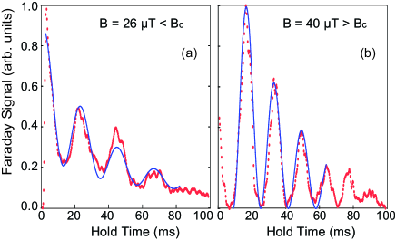
Figure 1: Faraday signal (proportional to $\langle F_{x}\rangle^{2}$) taken from a single measurement for $m=0$ at two magnetic fields, 26 $\mu$T and 40 $\mu$T starting with $\rho_{0}=0.5$, $\theta=0$. The solid line is a fit with a damped sinusoid. The signals show an oscillating phase (a) and a running phase (b) at $B$ below and above $B_{c}$, respectively, as evidenced by the signal reaching zero or not.

The single mode approximation (SMA) lett ; lyou1 is applied to understand our data. The spatial wavefunction of the BEC is treated as a single mode and the unit-normalized total wavefunction can be represented as $\Psi(\textbf{r},t)=\Phi(\textbf{r})(\sqrt{\rho_{-1}(t)}e^{i\theta_{-1}(t)},\sqrt{\rho_{0}(t)}e^{i\theta_{0}(t)},\sqrt{\rho_{+1}(t)}e^{i\theta_{+1}(t)})$, where $\rho_{m_{F}}$ and phases $\theta_{m_{F}}$ are independent of position. The Hamiltonian conserves particle number and $m$. The system is described using $\rho_{0}$ and $\theta=\theta_{-1}+\theta_{+1}-2\theta_{0}$, with the conserved classical spinor energy

$$E=E_{\rm qz}(1-\rho_{0})+c~{}\rho_{0}\left((1-\rho_{0})+\sqrt{(1-\rho_{0})^{2}-m^{2}}\cos\theta\right).$$ (1)

Here $E_{\rm qz}$ is the quadratic Zeeman shift ($E_{\rm qz}/h=(0.0277\,\textrm{Hz}/(\mu\textrm{T})^{2})B^{2}$), $c=c_{2}\langle n\rangle$ is the spin-dependent collision energy, and $c_{2}$ is $1.59\times 10^{-52}$ Jm³ for ²³Na lett . The evolution of $\rho_{0}$ and $\theta$ is given by $\dot{\rho_{0}}=-(2/\hbar)\partial E/\partial\theta$ and $\dot{\theta}=(2/\hbar)\partial E/\partial\rho_{0}$.

Figure 2 shows typical phase diagrams of the equal energy contours of Eq. 1 for $m=0$ at two magnetic fields. The preparation of the state determines the energy $E_{0}(B)$. Our initial states have $\theta=0$. At any magnetic field, we can define a separatrix, i.e. that energy contour, $E_{\rm sep}(B)$, on which there is a saddle point where $\dot{\rho_{0}}=\dot{\theta}=0$. This defines the boundary between two regions in phase space. In fact, $E_{\rm sep}(B)=E_{\rm qz}$ in our system.

When $E_{0}(B)>E_{\rm sep}(B)$, the value of $\theta$ is restricted, while for $E_{0}(B)<E_{\rm sep}(B)$ there is no bound. This defines regions with oscillating phase and running phase, respectively. In both regions $\rho_{0}$ oscillates. At $E_{0}(B)\gg E_{\rm sep}$, which corresponds to small magnetic fields, the period only weakly depends on the field. In the opposite limit, the period decreases rapidly with increasing field. In both cases, the oscillation is nearly harmonic. When $B\sim B_{c}$, defined by $E_{0}(B_{c})=E_{\rm sep}(B_{c})$, the oscillation is anharmonic and the period diverges for $B=B_{c}$.

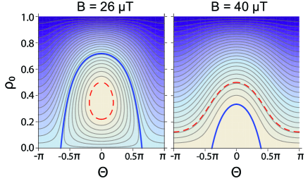
Figure 2: (Color online) Equal-energy contour plots generated from Eq. 1 at two magnetic fields, 26 $\mu$T (left) and 40 $\mu$T (right), with $m=0$ and $c/h=33$ Hz. The (red) dashed lines represent the energy of a state with $\rho_{0}(t=0)=0.5$. The heavy (blue) solid lines represent the energy of the separatrix ($E_{\rm sep}$) between oscillating and running phase solutions. Darker colors represent lower energies.

In the SMA, the Faraday signal is derived from

$$\langle F_{x}\rangle = \cos\left[\frac{\theta+(\theta_{+1}-\theta_{-1})}{2}\right]\sqrt{\rho_{0}\left(1+m-\rho_{0}\right)}$$

$$+\cos\left[\frac{\theta-(\theta_{+1}-\theta_{-1})}{2}\right]\sqrt{\rho_{0}\left(1-m-\rho_{0}\right)}.$$

The phase difference $\theta_{+1}-\theta_{-1}$ is determined by the fast Larmor precession and a slow evolution due to $\rho_{0}$ and $\theta$ lyou1 . For $m=0$, our Faraday signal is proportional to $\rho_{0}(1-\rho_{0})\cos^{2}(\theta/2)$. For oscillating phase solutions, $\theta$ oscillates about zero (with amplitude $<\pi$) and thus the signal is always greater than zero. On the other hand, the signal is periodically zero for running phase solutions. Figure 1 shows signals from the two regions. For $m\neq 0$, the signal is described by a more complicated expression, but the distinction between the two regions in the vicinity of $B_{c}$ remains the same.

These characteristics of the Faraday signal provide a sharp signature for locating $B_{c}$. Figure 3 shows the value of the minimum of the Faraday signal at different $B$ and $m$ after removal of the exponential decay. For the two magnetizations a transition from an oscillating phase solution with a non-zero minimum to a running phase solution with a minimum of zero, provides the sharp signature to locate $B_{c}$. In lett , the population oscillations were measured using SG-AI and fit by a sinusoid to extract a period and to locate the two regions of phase space. No sharp experimental signature distinguishing the boundary was observed.

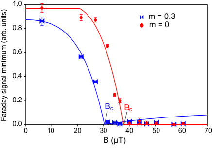
Figure 3: (Color online) The minimum of the Faraday signal as a function of magnetic field for $m=0$ (red dots) and $m=0.3$ (blue bowties). A scale factor is applied to the Faraday signal to correct for the PD response at different $f_{L}$. The lines are fits based on Eq. Quantum Phase Transitions and Continuous Observation of Spinor Dynamics in an Antiferromagnetic Condensate, which yield the fit parameters $\rho_{0}=0.42$ and $N=1.50\times 10^{5}$ for $m=0$, and $\rho_{0}=0.54$ and $N=1.32\times 10^{5}$ for $m=0.3$. The fit parameters are within the 3% uncertainty of those derived from absorption images.

Figure 3 also shows a comparison between the prediction from the SMA and the data. For $m=0$, the agreement is excellent. For $m=0.3$, however, the prediction does not agree with our measurements for fields significantly larger than $B_{c}$. At the transition point, the minimum of the Faraday signal goes to zero, but above this point, the theory predicts that the minimum rises with $B$, even though the solution has a running phase. This increase is not observed. The apparent agreement between the SMA theory and our measurements has been surprising - at every magnetic field reported in this paper, we have seen the presence of several spatial modes/spin domains during the spin oscillations, although not in steady-state. The observation of spin domains is in marked contrast to our previous work lett . Several technical changes may have contributed to the domain formation, such as a 50% increase of the total atom number and more stable magnetic bias fields. Understanding the ways in which multiple spatial modes and domains affect the spin dynamics is an interesting direction for future research.

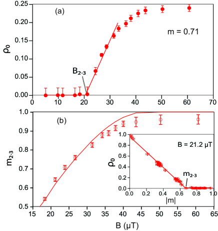
Figure 4: Evidence of phase transitions in the mean-field ground state of the antiferromagnetic spinor BEC. (a): Points with uncertainties indicate $\rho_{0}$ as a function of $B$ at $m=0.71(2)$. The intersection of two linear fits defines $B_{2-3}$, the critical magnetic field for the phase transition. (b) Inset: $\rho_{0}$ versus $m$ for $B=21.2~{}\mu$T. The intersection of two linear fits defines $m_{2-3}$, the critical magnetization. The main figure shows $m_{2-3}$ versus $B$. The solid line is the prediction from the SMA.

At long times, after the oscillations have damped out, we can study the mean-field ground state of this system. Within the SMA, a quantum phase transition from a three- to a two-component BEC is predicted for the mean-field ground state gs . We use SG-AI as a direct way to measure the equilibrium populations and to observe this phase transition.

The behavior of the variance of $\rho_{0}$ allows us to determine when the system has settled down to a steady state. At a given time we measure $\rho_{0}$ 25-30 times and calculate a variance. In the steady state, the variance reaches a minimum. Due to technical noise in atom counting, this variance is larger than that predicted by a quantum calculation of the spinor ground state youQ . We find that a steady state for $m=0$ is reached within our maximum hold time of 10 s for $B\geq 18~{}\mu$T. For non-zero $m$, the steady state is reached within a much shorter time.

Figure 4 (a) shows the steady state values of $\rho_{0}$ as a function of $B$. For each measurement, we prepare nearly identical initial states at $B=24.4~{}\mu$T to set the populations and magnetizations. We then wait 4 s to reach the steady state before adiabatically ramping the field to a desired final value over 500 ms. We then wait another 5s before making an SG-AI measurement. In the inset of Fig. 4 (b), however, each initial state is directly prepared with a different magnetization. In both figures, a transition between a two-component BEC with $\rho_{0}=0$ and a three-component BEC with non-zero $\rho_{0}$, is observed. A critical magnetic field $B_{2-3}$ and a critical magnetization $m_{2-3}$ are defined and extracted from the intersection of two linear fits to the data. Good agreement is found between the experimental value of $m_{2-3}$ and the prediction from the SMA gs , as shown in Fig. 4(b). This confirms a phase transition from a three- to a two-component spinor BEC in the antiferromagnetic mean-field ground state. Although it is observed here at a finite temperature the phase transition should remain at zero temperature, where the transition would be driven solely by quantum fluctuations. It has been predicted that this phase transition persists even when the three spin states do not share the same spatial distribution and the application of the SMA is no longer appropriate gs .

In conclusion, we have demonstrated that Faraday rotation spectroscopy provides a method to continuously monitor the spin dynamics in an antiferromagnetic spinor BEC. The technique provides a sharp signature to locate the magnetically tuned boundary in phase space between the oscillating and running phase solutions. We observe a dependence of the position of this separatrix on the magnetization. In addition, we have confirmed a quantum phase transition from a two- to a three-component BEC in the mean-field ground state. We are presently investigating the dissipation mechanism leading to the equilibrium observed in these experiments. We think that physics beyond the SMA, possibly similar to Landau damping of excitations of a single component BEC landau , may explain the dissipation.

We thank W. D. Phillips, J. V. Porto and E. Gomez for insightful discussions, and ONR for financial support. SEM thanks the NIST/NRC postdoctoral program.

References

- (1) L. Guttman and J. R. Arnold, Phys. Rev. 92, 547 (1953).
- (2) C. J. Myatt et al., Phys. Rev. Lett. 78, 586 (1997).
- (3) M. S. Chang et al., Nature Physics 1, 111 (2005).
- (4) M. S. Chang et al., Phys. Rev. Lett. 92, 140403 (2004).
- (5) W. Zhang et al., Phys. Rev. A 72, 013602 (2005).
- (6) J. Stenger et al., Nature 396, 26 (1998).
- (7) H. J. Miesner et al., Phys. Rev. Lett. 82, 2228 (1999).
- (8) A. T. Black et al., Phys. Rev. Lett. 99, 070403 (2007).
- (9) A. Widera et al., New J. Phys. 8, 152 (2006).
- (10) T. Kuwamoto et al., Phys. Rev. A 69, 063604 (2004).
- (11) H. Schmaljohann et al., Phys. Rev. Lett. 92, 040402 (2004).
- (12) J. Kronjager et al., Phys. Rev. Lett. 97, 110404 (2006).
- (13) W. Zhang, S. Yi and L. You, New J. Phys. 5, 77 (2003).
- (14) M. Vengalattore et al., Phys. Rev. Lett. 100, 170403 (2008).
-
(15)
J. M. Higbie et al., Phys. Rev.
Lett. 95, 050401
(2005);
Y. J. Wang et. al, Phys. Rev. Lett. 94, 090405 (2005);
M. H. Wheeler et al., Phys. Rev. Lett. 93, 170402 (2004);
M. Saba et al., Science 307, 1945 (2005). - (16) G. A. Smith, S. Chaudhury, and P. S. Jessen, J. Opt. B 5, 323 (2003).
- (17) M. L. Terraciano et al., Phys. Rev. A 77, 063417 (2008).
- (18) P. C. D. Hobbs, Applied Optics 36, 903 (1997).
- (19) G. A. Smith et al., Phys. Rev. Lett. 93, 163602 (2004).
- (20) L. Chang et al., Phys. Rev. Lett. 99, 080402 (2007).
- (21) L. Pitaevskii and S. Stringari, Phys. Lett. A 235, 398 (1997).