Phase-Space Networks of Geometrical Frustrated Systems

Abstract

Geometric frustration leads to complex phases of matter with exotic properties. Antiferromagnets on triangular lattices and square ice are two simple models of geometrical frustration. We map their highly degenerated ground-state phase spaces as discrete networks such that network analysis tools can be introduced to phase-space studies. The resulting phase spaces establish a novel class of complex networks with Gaussian spectral densities. Although phase-space networks are heterogeneously connected, the systems are still ergodic except under periodic boundary conditions. We elucidate the boundary effects by mapping the two models as stacks of cubes and spheres in higher dimensions. Sphere stacking in various containers, i.e. square ice under various boundary conditions, reveals challenging combinatorial questions. This network approach can be generalized to phase spaces of some other complex systems.

I 1. Introduction

One challenge to understanding disordered solids is the complex geometry of their phase spaces, including the relative positions and interconnections between the different metastable states. Phase spaces are usually too large and complicated to be directly studied. For example, an $N$-particle system typically has a vast abstract $6N$-dimension phase space ($3N$ for position, $3N$ for velocity). Here, we propose that some simple models of disordered solids, such as geometrical frustrated spin models, provide an ideal platform for phase-space studies. Their phase spaces can be mapped as nontrivial complex networks, so that the recently developed large tool box of network analysis Albert02 ; Newman03 ; Costa07 can be used to understand phase spaces. On the other hand, these phase spaces provide a new class of complex networks with novel topologies.

When a system has competing interactions, there is no way to simultaneously satisfy all interactions, a situation known as frustration. Frustration widely exists in systems ranging from neural networks to disordered solids. Frustration can also arise in an ordered lattice solely from geometric incompatibility Moessner06 . For example, consider the three antiferromagnetic Ising spins on the triangle shown in Fig. 1A. Once two of them are antiparallel to satisfy their antiferromagnetic interaction, there is no way that the third one can be antiparallel to both of the other two spins. Frustration leads to highly degenerated ground states and, subsequently, to complex materials with peculiar dynamics such as water ice Pauling35 , spin ice Bramwel01 , frustrated magnets Bramwel01 , artificial frustrated systems Wang06 and soft frustrated materials Han08 .

In geometrical frustrated systems, spins on lattices have discrete degrees of freedom, such that their phase spaces are discrete and can be viewed as networks. A node in the network corresponds to a state of the system. Two nodes are connected by an edge (i.e. a link) if the system can directly evolve from one state to the other without passing through intermediate states. Edges are undirected because dynamic processes at the microscopic level are time reversible. The challenge is how to construct and analyze such large phase-space networks. For example, how do we identify whether or not two nodes are connected?

II 2. Antiferromagnets on triangular lattices.

The first model we consider is antiferromagnetic Ising spins on a two-dimensional (2D) triangular lattice Wannier50 . For a large system with periodic boundary conditions, it has $\sim e^{0.323N_{spin}}$ degenerated ground states where $N_{spin}$ is the number of spins Wannier50 . For example, configuration 3A in Fig. 1C is one ground state in the hexagonal area. We refer to pairs of neighbouring spins in opposite states as satisfied bonds, i.e., they satisfy the antiferromagnetic interaction. Since one triangle has at most two satisfied bonds (see Fig. 1A), the ground state should have 1/3 of its bonds frustrated and 2/3 of its bonds satisfied Wannier50 . If we plot only satisfied bonds, a ground state can be mapped to a random lozenge tiling Blote94 , see configuration 3A in Fig. 1C. A lozenge is a rhombus with $60^{\circ}$ angles. By colouring lozenges with different orientations with different grey scales, the tiling can be viewed as a stack of 3D cubes, or as a simple cubic crystal surface projected in the [1,1,1] direction Blote94 , see Fig. 1C.

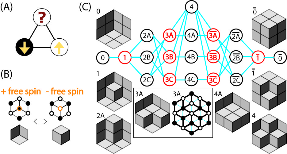
Figure 1: A phase-space network of cube stacks. (A): Three antiferromagnetic spins on a triangle cannot simultaneously satisfy all their interactions. (B): The central spin has three up and three down neighbours, so that it can flip freely without energy change. Satisfied bonds can be viewed as cubes. The +/- free spin flip corresponds to adding/removing a cube. (C): The $2\times 2\times 2$ cube stacks are stable against gravity along the [1,1,1] direction. Stack configurations have one-to-one correspondence to Ising ground states under ‘hexagon boundary condition’, e.g., see configuration 3A. In the right 3A configuration, the black lines are satisfied bonds forming rhombuses and the blue lines are frustrated bonds. In total, there are 20 legal stacks, i.e., 20 nodes in the phase-space network. The network is bipartite, i.e., consisting of alternating red (even number of cubes) and black (odd number of cubes) states.

The ground state has a local zero-energy mode, as shown in Fig. 1B: the central particle can flip without changing the energy since it has 3 up and 3 down neighbours. The system can evolve via a sequence of such single spin flips, even at zero temperature. We call such a local zero-energy mode the basic flip. Any configuration change can be viewed as a sequence of such basic flips. Recently, we directly observed such flips in a colloidal monolayer Han08 . In the language of cubes, a basic flip is equivalent to adding or removing a cube, see Fig. 1B. By continuing to add or remove one cube from the stack surface, we can access all possible stack configurations in the large box. Thus, the ground-state phase space is connected by this ‘hexagonal boundary condition’. The corresponding cube stacking in a large box is equivalent to the boxed plane partition problem in combinatorics Andrews04 . The total number of ways to stack unit cubes in an $L^{3}$ box is given by the MacMahon formula: MacMahon

$$N_{n}(L) = \prod_{1\leq i,j,k\leq L}\frac{i+j+k-1}{i+j+k-2}=\frac{H^{3}(L)H(3L)}{H^{3}(2L)}$$ (1)

$$\sim \left(\frac{27}{16}\right)^{\frac{3}{2}L^{2}}\textrm{when }L\to\infty,$$

where the hyperfactorial function $H(L)=\prod_{k=0}^{L-1}k!$. The first several $N_{n}(L=2,3,4,5,\cdots)$ are 20, 980, 232848, 267227532,$\cdots$ (see the number sequence A008793 in ref. sequence ). When $L=2$, all 20 ground-state configurations in Fig. 1C have the same minimum possible energy, i.e., 12 frustrated bonds in 12 rhombuses.

III 3. Network properties.

The 20-node phase-space network shown in Fig. 1C can be constructed based on the following two facts: (1) Spins have discrete degrees of freedom, such that the phase space is a discrete network; (2) Any configuration change can be decomposed to a sequence of basic flips. Consequently, we can define an edge between two nodes if the two states differ by only one basic flip (i.e., one cube), such that the system can directly change from one node to the other without passing through intermediate nodes.

Numerically, we can handle networks only up to $L=4$ stacks with $N_{n}=232848$ nodes; nevertheless many general properties have emerged from such small systems. Figure 2A shows the connectivity (i.e. degree) distribution Albert02 ; Newman03 ; Costa07 of cube-stack networks. The connectivity, $k_{i}$, is the number of edges incident with the node $i$. The connectivities of various frustrated systems appear to have Gaussian distributions (see Fig. 2). This behavior is similar to that of small-world networks Watts98 ; Costa07 and Poisson random networks Newman03 ; Costa07 and different from that of scale-free networks Costa07 ; Barabasi99 .

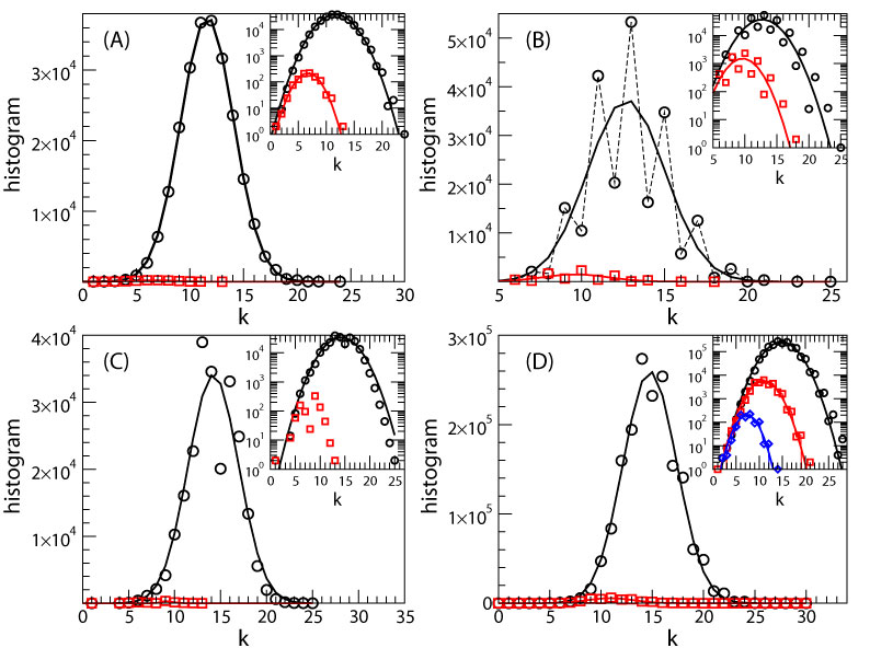
Figure 2: Connectivity distributions. Histograms of the connectivities of ground-state phase-space networks for (A) antiferromagnets on triangular lattices, and (B, C, D) square ices under different boundary conditions. (A): $L=4$ (circles) and $L=3$ (squares) cube stacks. (B): Spheres stacks in $L=6$ (circles) and $L=5$ (squares) tetrahedra. (C): Spheres stacks in $L=4$ (circles) and $L=3$ (squares) octahedra. (D): Sphere stacks in $L=6$ (circles), $L=5$ (squares) and $L=4$ (diamonds) containers shown in Fig. 11. Insets: semi-log plots. The curves in the main plots and insets show the best Gaussian fits.

Other network properties, such as the diameter and the cluster coefficient, can be readily derived from the cube stack picture. The shortest path length between two nodes is simply the number of different sites among all the $L^{3}$ sites. The largest distance, i.e. the diameter of the network, is $L^{3}$ between the ‘vacant’ and the ‘full’ states. Here, we define the vacant state as no cube (i.e., $L^{3}$ vacant sites) and the full state as no vacant site (i.e., $L^{3}$ cubes). The networks have small-world properties Watts98 ; Costa07 in the sense that the diameter, $L^{3}$, is almost logarithmically small compared with the network size, $\sim e^{N_{spin}}\sim e^{L^{2}}$. The network is bipartite (see the black and red circles in Fig. 1C) because a cube stack comes back to its initial configuration only by adding and removing the same number of cubes, i.e., an even number of basic flips. Consequently, the cluster coefficient Costa07 , which characterizes the density of triangles in the network, is 0.

Spectral analysis provides global measures of network properties. For an $N_{n}$-node network, the connectivity (or adjacent) matrix $\mathbf{A}$ is an $N_{n}\times N_{n}$ matrix with $A_{ij}=1$ if nodes $i$ and $j$ are connected, and zero otherwise. Since edges in phase-space networks are undirected, $\mathbf{A}$ is symmetric and all its eigenvalues, $\lambda_{i}$, are real. The spectral density of the network is the probability distribution of these $N_{n}$ eigenvalues: $\rho(\lambda)=\frac{1}{N_{n}}\sum_{i=1}^{N_{n}}\delta(\lambda-\lambda_{i})$. $\rho(\lambda)$’s $q$th moment, $M_{q}$, is directly related to the network’s topological feature. $D_{q}=N_{n}M_{q}=\sum_{i=1}^{N}(\lambda_{i})^{q}$ is the number of paths (or loops) that return back to the original node after $q$ steps Costa07 . In a bipartite network, all closed paths have even steps so that all odd moments are zero. Consequently, the spectral density is symmetric and centered at zero. The $i$th node with $k_{i}$ neighbours has $k_{i}$ ways to return back after two steps; hence, the variance $\sigma^{2}=M_{2}=\sum_{i}k_{i}/N_{n}=\bar{k}$, where $\bar{k}=2N_{edge}/N_{n}$ is the mean connectivity. We rescale the spectral densities by $\bar{k}^{1/2}$ to the unit variance (see Fig 3). The rescaled spectral densities of different frustration models collapse onto the same Gaussian distribution. By counting $D_{q}$, we show that spectral densities are Gaussian at the infinite-sized limit (see Section I of Supplementary Information (SI)). This distinguishes phase spaces from other complex networks. For example, the spectral density of a random network is the semicircle in Fig. 3. The spectral densities have triangular distributions for scale-free networks and irregular distributions for small-world, modular hierarchical and many real-world networks deAguiar05 ; Farkas01 .

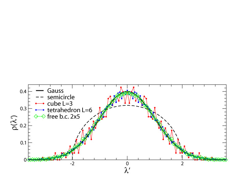
Figure 3: Spectral densities of phase-space networks. Variances are rescaled to 1 by $\lambda^{\prime}=\lambda/\bar{k}^{-\frac{1}{2}}$. Black curve: Gaussian distribution $e^{-\lambda^{\prime 2}/2}/\sqrt{2\pi}$. Dashed curve: Wigner’s semicircle law for random networks. $\rho(\lambda)=\sqrt{4\sigma^{2}-\lambda^{2}}/(2\pi\sigma^{2})$ if $|\lambda|<2\sigma$ and zero otherwise. The variance $\sigma^{2}$ is also rescaled to 1. Red curve: the spectral density of the 980-node network of $L=3$ cube stacks. Blue curve: the 7436-node network of $L=6$ sphere stacks in a tetrahedron, i.e., $7\times 7$ square ice under the domain wall boundary condition. Green curve: 7782-node network of $2\times 5$ square ice under the free boundary condition. Their Gaussian fits are indistinguishable from the black curve.

Spectral analysis can also detect the network’s community (or modular) structures Newman06PNAS if there are any. The algorithm in ref. Newman06PNAS identifies some relatively highly connected subnetworks (i.e., communities). However, we still observe a number of edges between subnetworks such that the whole phase space has to be considered as fully ergodic. Our simulation shows that the system can easily travel through the whole phase-space network via basic flips and will not be trapped in a local community for a long time.

IV 4. Poisson processes and equal probability in phase spaces.

The fundamental assumption of statistical mechanics is that the dynamic trajectory of a system wanders through all its phase spaces and spends the same amount of time in each equally sized region of the phase space. However, this ‘equal a priori probability postulate’ (essentially the same as the ‘ergordic hypothesis’ Patrascioiu87 ) is not necessarily true, as Einstein noted Cohen07 . How the system moves from one configuration to the next depends on the details of the molecules’ interactions (e.g. nearest-neighbor antiferromagnetic interactions here); these microscopic dynamics may make some configurations more likely than others.

Network analysis provides an opportunity to study ergodicity. Unlike billiards with deterministic trajectory, we assume the spin flipping is due to the random thermal motion and not depends on history. Thus the dynamical evolution of the system can be viewed as a random walk on its phase-space network. It still interesting to ask whether this random walk can uniformly visit each node given the complex topology of the network. In another word, whether the system can visit each possible microstate configuration under the complex constraint of local nearest-neighbor interactions.

Random walks on a network are rather chaotic, and nodes with higher connectivities will be visited more frequently. Thanks to the theorem in ref.Noh04 , the mean visiting frequency for node $i$ is $k_{i}/N_{edge}$, which only depends on local connectivity, $k_{i}$, and does not depend on the global structure of the network. Here, $N_{edge}$ is the total number of edges. This theorem is a direct consequence of the undirectedness of edges. Although highly connected nodes are visited more frequently ($\sim k_{i}$), interestingly, the equal-probability postulate does not break down because the average time stayed at node $i$ is $\sim 1/k_{i}$. Basic flips are random and independent of history, meaning that it is a Poisson process. We define the flipping probability of a basic flip within a unit of time as $\nu$, which is the intensity of the Poisson process. In Poisson processes, the time interval between flips (i.e., the staying time) has an exponential distribution, $e^{-\nu t}$, and the mean staying time is $1/\nu$. Note that multiple flips will not flip exactly simultaneously because time is continuous. Therefore we do not need to worry about possible illegal configurations if neighbor free spins flip simultaneously. For a node with connectivity $k$, the superposition of $k$ Poisson processes is still a Poisson process with intensity $k\nu$ and, consequently, the mean staying time is $1/(k\nu)$. A random walker has higher frequency ($\sim k$) to visit a high-$k$ node, but will stay there for a shorter time ($\sim 1/k$), so that the equal-probability postulate is recovered. Boltzmann assumed that molecules shift from one microscopic configuration to the next in such a way that every possible arrangement is equally likely, i.e., all edges have the same weight. We find that the equal-probability postulate still holds if edges have different weights (see Appendix B), which, for example, can represent different potential barriers in complex energy landscapes in phase spaces.

V 5. Square ice.

We further study another frustration model called square ice to identify the more general properties of phase spaces. Square ice is the two-dimensional version of water ice as shown in Fig. 9. It can be viewed as jigsaw tiling Bressoud99 or spin ice Bramwel01 ; Bressoud99 ; Wang06 ; Propp01 (see Figs. 4A,D). Oxygen atoms are represented by vertices and the relative directions of hydrogen atoms are represented by arrows. The ground state of the system follows the ice rule, i.e., each vertex has two incoming and two outgoing arrows. It is also known as the six-vertex model since each vertex has six possible configurations (i.e., six types of jigsaw tiles). For a vertex associated with four ferromagnetic spins, frustration is inevitable (see the example in Fig. 4C).

Flipping a closed loop of arrows from clockwise to counterclockwise (or vice versa) does not break the ice rule. The smallest four-spin loops in Figs. 4D,G are labeled in red (clockwise) and yellow (counterclockwise). They are basic flips since any configuration change can be decomposed as a sequence of such flips Eloranta99 . Similar to cube stacking, all the legal configurations of square ice are connected via basic flips Eloranta99 . Consequently, the phase-space network of square ice can be constructed.

The square ices in Figs. 4A,D have domain wall boundary conditions (DWB) as shown by the black arrows in Fig. 4D. There is a one-to-one correspondance between jigsaw tiling with DWB and alternating sign matrices (ASM) Bressoud99 (see Fig. 4A). ASM are square matrices with entries 0 or $\pm$1 such that each row and column has an alternating sequence of +1 and -1 (zeros excluded) starting and ending with +1. The number of $n\times n$ ASM is Bressoud99

$$W = \prod_{1\leq i\leq j\leq n}\frac{n+i+j-1}{2i+j-1}=\prod_{j=0}^{n-1}\frac{(3j+1)!}{(n+j)!}$$ (2)

$$\sim \left(\frac{27}{16}\right)^{\frac{n^{2}}{2}}\textrm{when }n\to\infty,$$

i.e., the number of nodes of the phase-space network of an $n\times n$ square ice with DWB.

VI 6. Mapping square ices to sphere stacks.

Mapping 2D triangular antiferromagnets to 3D cube stacks greatly simplifies the picture of the phase space and allows combinatorial analysis to generate quantitative results such as Eq. 1 and Gaussian spectral densities. Here, we show that square ices can be mapped to 3D close-packed spheres in face-centered cubic (FCC) lattices. Each square plaquette in Figs. 4D,G is assigned a height Beijeren77 ; Eloranta99 based on the rule shown in Fig. 4B: When walking from the plaquette with height $h$ to its neighbor, the height increases by 1 if it crosses a left arrow and decreases by 1 if it crosses a right arrow. The ice rule guarantees that the height change around a vertex is zero and $h$ is independent of the path along which it was computed. From the minimum and maximum possible heights, we found that DWB yields a stack of building blocks in a tetrahedron (see Fig. S5 of SI). A plaquette can be flipped only when its four neighbor plaquettes have the same height. Since each building block is ‘supported’ by four underneath blocks in an effective ‘gravity field’, the stack can be viewed as an FCC lattice along the [100] direction, see section III of SI. Thus, the stacking blocks should be rhombic dodecahedra, which are primitive unit cells of FCC lattices. FCC lattices can be conveniently represented by close-packing of spheres. Sphere stacks in side length $L$ tetrahedra have one-to-one correspondence to $(L+1)\times(L+1)$ square ices with DWB (see Fig. S5 of SI). The stack of red spheres in Fig. 4E corresponds to the configurations in Figs. 4A,D. The physical heights of the red spheres on the top surface are the heights of the corresponding plaquettes in the square ice. At the interface between the red spheres and the yellow vacant sites, the four removable red spheres on the top surface correspond to the red plaquettes and the four addable yellow sites correspond to the yellow plaquettes in Fig. 4C. Similar to the cube stacking, here, a basic flip from counterclockwise to clockwise (or vice versa) corresponds to adding (or removing) a sphere. By adding spheres from the vacant state shown in Figs. 10A,G, we can generate all possible stack configurations, i.e., all the nodes of the phase-space network. Similar to the cube stack case, we can construct the phase-space network of sphere stacks by adding an edge between two nodes if the two stacks are different by one sphere.

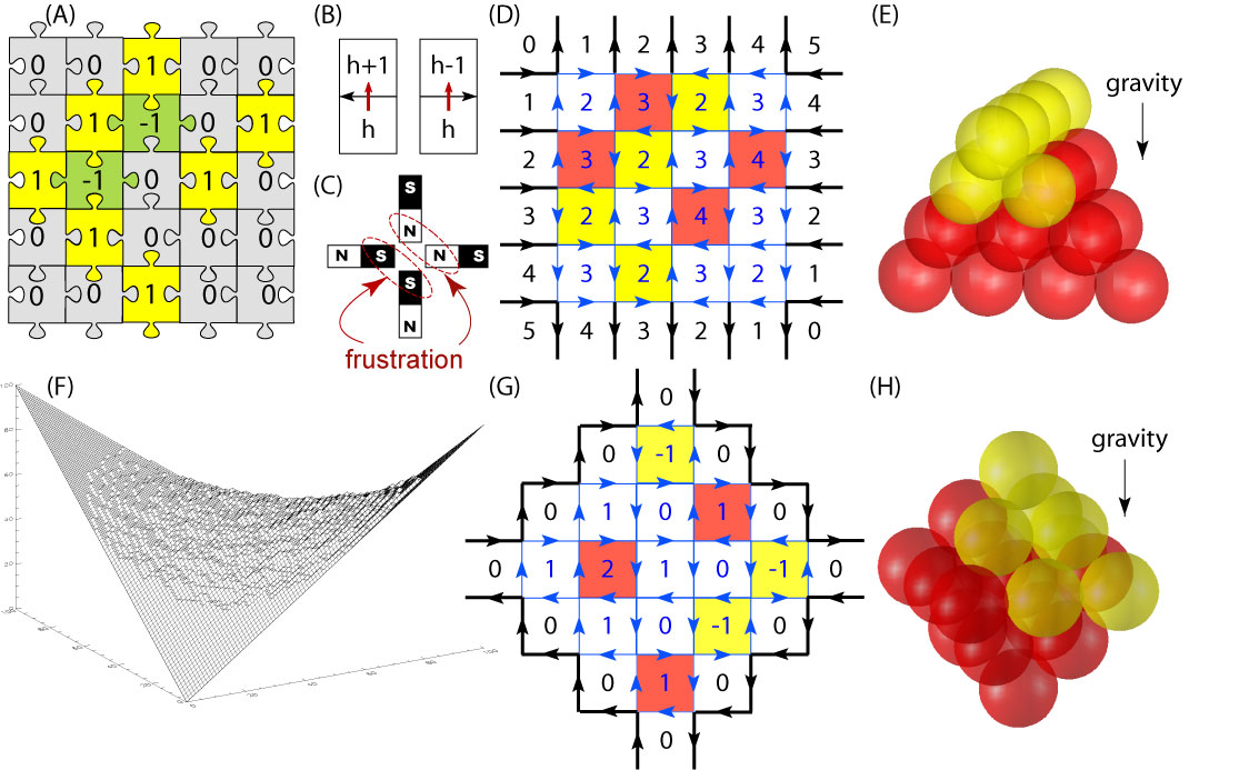
Figure 4: Square ice. (A): A $5\times 5$ square ice under the domain wall boundary condition. Each jigsaw tile can be viewed as a water molecule with one oxygen atom in the center and two hydrogen atoms at the two bulges (see Fig. S4 of SI). By assigning vertical tiles to be 1, horizontal tiles to be -1 and the other four types to be 0, a $5\times 5$ alternating sign matrix Bressoud99 is obtained. (B): The height rule used in (D) and (G). (C): Four magnets placed at a cross inevitably have frustrations. (D): The spin ice mapped from (A). The arrows represent bulge directions in (A). The blue arrows may flip under the ice rule. Each plaquette is assigned a height based on the rule in (B). The upper left corner is defined as height zero. Basic flips (i.e., four-arrow loops) are labeled in red (clockwise) and yellow (counterclockwise). (E): The corresponding sphere stack of (D). Yellow spheres are vacant sites. (F): A typical sphere stack in an $L=100$ tetrahedron. The sphere centers are connected so that it appears to be a stack of polyhedra. (G): A spin ice configuration in an Aztec diamond area under the constant-height boundary condition. (H): The corresponding sphere stack of (G) in an octahedron.

VII 7. Network properties of sphere stacks.

We numerically studied phase-space networks of small square ices under various boundary conditions. Our largest network contains 2068146 nodes and 13640060 edges ($4\times 5$ ice under free boundary conditions). All networks have the small-world property. Their connectivity distributions in Figs. 2B,C,D and the spectral densities in Fig. 3 are similar to those of cube stacks. Apparently, both cube-stack and sphere-stack phase spaces have Poisson processes with equal probability and Gaussian spectral densities.

VIII 8. Boundary effects.

Stacks in higher dimensions provide a vivid means for qualitative visualization of the boundary effect, which has not been well understood in geometrical frustration Millane04 . One peculiar property of geometrical frustration is that boundary effects often percolate through the entire system even in the infinite-sized limit Millane04 ; Destainville98 . This can be visualized from a typical sphere stack in the $L=100$ tetrahedron shown in Fig. 4F, which has a central disordered region and four frozen (ordered) corners known as the arctic circle phenomenon Jockush98 . The disordered region is not uniformly random since different positions have different mean surface curvatures and entropy densities Destainville98 (see Appendix C). Consequently, the infinitely large limit under DWB cannot be called the thermodynamic limit due to the lack of homogeneity.

Different boundary conditions in square ice correspond to different container shapes in sphere stacking. For example, the boundary condition shown in Fig. 4G corresponds to sphere stacks in an octahedron (see Fig. 4H) because the lowest possible heights form an inverted pyramid (i.e. the container) and the highest heights form an upright pyramid (i.e. the lid). Appendix D shows another boundary condition whose container and lid have different shapes. At a given boundary condition, the lid and the container form an interesting pair of dual surfaces. Some boundary conditions do not have the arctic circle phenomenon, as illustrated by the sphere stacking in Appendix C.

We found that phase spaces are ergodic under free or fixed boundary conditions, but nonergrodic under periodic boundary conditions whose networks consist of disconnected subnetworks. As an example, Fig. 5 is the phase-space network of the $2\times 3$ square ice wrapped on toroid, i.e., under periodic boundary conditions. It contains two nontrivial (12-node) subnetworks and 20 trivial isolated nodes. The corresponding 44 configurations are shown in Fig. 14. For $m\times n$ periodic square ice wrapped on a toroid, we show that its phase space contains $2^{n+1}+2^{m+1}-4$ trivial isolated nodes, $(m-1)\times(n-1)$ nontrivial subnetworks and the smallest non-trivial subnetwork has $\frac{(m+n-1)!}{(n-1)!(m-1)!}$ nodes (see Appendix E). These results are confirmed numerically.

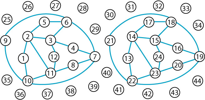
Figure 5: The phase-space network of $2\times 3$ square ice under periodic boundary conditions. There are 44 possible states (see their detailed configurations in Figs. S9A,B of SI). States 1 to 12 are connected via basic flips; states 13 to 24 are connected; and states 25 to 44 do not contain any basic flips, thus they are isolated nodes.

IX 9. Discussion and outlook.

We build novel connections between geometrical frustration, combinatorics (e.g., plane partition and sphere stacking) and complex networks to exploit open questions and analysis tools from these fields. Other frustration models, such as triangular and kagomé ices, antiferromagnets in 2D kagomé and 3D pyrochlore lattices Moessner98 ; Lee02 , have height functions and basic flips so that their phase-space networks can be similarly constructed. In principle, these models can be mapped to polyhedra stacking in higher dimensions, so that their rich symmetries and boundary effects become more transparent.

Quasicrystals can also be mapped to higher-dimensional lattices. Projecting the high-dimensional lattices to lower dimensions could result in periodic lattices (i.e., geometrical frustration) at certain projection angles, or aperiodic structures (i.e., quasicrystals) at other angles. Phasons in quasicrystals correspond to basic flips in geometrical frustration Destainville98 , thus similar phase-space analysis may be applied to quasicrystals. In fact, the infinitely degenerated ($\sim e^{N}$ where $N\to\infty$) ground states in both geometrical frustration and quasicrystals are essentially metastable states since the third law of thermodynamics dictates that the true ground state of real materials must have finite degeneracy. Network analysis may provide a possible approach to understanding the observed glassy dynamics in frustrated systems Han08 . At finite temperatures, phase-space networks can be similarly constructed. The nodes are all configurations on the hypersurface in the phase space determined by the conservation laws. Configurations change via basic flips and diffusion of thermal excitations Han08 ; Blunt08 . These motions are represented by edges. The weight of each edge can be assigned by a Boltzmann factor or defined by the physical details of the real system Blunt08 . Height representation can be recovered by assigning vector heights Moore00 , so that systems at finite temperatures might be mapped to stacks in even higher dimensions.

Compared with intensively studied social networks, information networks, biological networks and technological networks Newman03 , phase-space networks belong to a new class with unique Gaussian spectral densities. A large tool box Costa07 has been developed in the recent decade to study network dynamics, correlations, centrality, community structures, fractal properties Song05 , coarse graining Gfeller07 , etc. These tools can be readily applied to phase-space studies. In particular, phase spaces might have fractal structures because stacks of cubes or spheres have self-repeating patterns on various length scales. This may cast new light on the highly controversial Tsallis’s nonextensive entropy Cho02 ; GellMann04 , which is based on the assumption that nonequilibrium systems have fractal phase spaces. To date, a real example to support this assumption has not been available. Indeed, geometrical frustrated ground states share the same features as the long-range interacting systems typically discussed in the context of Tsallis entropy. One example is boundary effects percolating through the entire system so that the system is not uniform at the infinite-sized limit and cannot be viewed as a simple sum of its subsystems (i.e., non-extensive).

In statistical physics, the two models we studied here are considered as exactly solvable Baxter82 under periodic boundary conditions at the infinite-sized limit. Combinatoric analysis, although challenging, provides an alternative approach to yield exact results about finite systems and at various boundary conditions. Cube stacking (i.e., rhombus tiling or plane partition Bressoud99 ), naturally appears in many chemical and physical problems, such as counting benzenoid hydrocarbons, percolation, crystal melting and string theory Okounkov03 . In contrast to the intensively studied cube stacking, sphere stacking has not been explored. Only some combinatoric properties of sphere stacking in tetrahedra are available since we can map them to ASM. Our numerical calculations show that there are $2,7,42,429,7436,218348\cdots$ ways to pack spheres in $L=1,2,3,4,5,6,\cdots$ tetrahedra; and $2,18,868,230274,\cdots$ ways in $L=1,2,3,4,\cdots$ octahedra. The former number sequence (i.e., sequence A005130 in ref.sequence ) is given by Eq. 2, while the formula for the latter is not available. Moreover, many questions studied in cube stacking can be asked about FCC sphere stacking. For example, how many ways are there to pack $N$ spheres into a tetrahedron? Is there a similar generating function as cube stacking for sphere stacking in a tetrahedron MacMahon ? What is the ensemble-averaged surface in Fig. 6A, i.e., what are the entropy density distributions at the infinite-sized limit Destainville98 ; Kenyon07 ? These questions can also be asked about other container shapes. Furthermore, square ice has one-to-one mappings to other 2D models, such as three-color graphs, dimers, fully packed loops, etc. Propp01 . It also has one-to-multiple mapping to the domino tiling Elkies92 . Sphere stacking provides a simple 3D picture and casts new light on these 2D models.

X Acknowledgements

We thank Michael Wong for helpful discussions.

XI Appendix A: Proof of the Gaussian spectral density

The characteristic function, i.e., the Fourier transform of the probability function, uniquely describes a statistical distribution. It can be written as a series of moments of the distribution. Hence, to prove that the spectral density is Gaussian, we only need to show that all orders of the moments are the same as those of a Gaussian distribution. For a Gaussian distribution centered at 0, its odd moments are zero and its even moments (of order $q$) are $M(q)=\frac{(q)!}{2^{q/2}(q/2)!}\sigma^{q}=(q-1)!!\sigma^{q}$, where $\sigma^{2}$ is the variance. For an $N_{n}$-node undirected network, $D(q)=N_{n}M(q)$ is the number of directed paths that return to their starting node after $q$ steps Costa07 . We count $D_{q}$ by stacking cubes/spheres and show that $M(q)=D(q)/N_{n}$ follows the Gaussian $M(q)$.

The phase-space networks are bipartite since walking an odd number of steps (i.e., adding/removing cubes/spheres an odd number of times) cannot return back to the original state. Consequently, all odd moments are zero, i.e., the distribution is symmetric and centered at 0. $D(2)$ is the number of ways to have one basic flip, $f_{1}$, and its reverse flip, $\bar{f}_{1}$. Given a stack configuration, $i$, with $k_{i}$ available basic flips, i.e., node $i$ with connectivity $k_{i}$ in the phase-space network, its $D(2)_{i}=k_{i}$. Thus, the total $D(2)=\sum_{i}k_{i}=N_{n}\bar{k}$ where $\bar{k}=2N_{edge}/N_{n}$ is the mean connectivity. Compared with the second moment, $M(2)=\sigma^{2}$, we have $\bar{k}=\sigma^{2}$. $D(4)$ is the number of ways to have two basic flips, $f_{1}$, $f_{2}$, and reverse flips, $\bar{f}_{1}$, $\bar{f}_{2}$. Subscripts 1 and 2 denote the time order. Given $f_{1}$ and $f_{2}$, typically there are three ways to arrange them in legal order: $f_{1}$-$\bar{f}_{1}$-$f_{2}$-$\bar{f}_{2}$, $f_{1}$-$f_{2}$-$\bar{f}_{1}$-$\bar{f}_{2}$ and $f_{1}$-$f_{2}$-$\bar{f}_{2}$-$\bar{f}_{1}$. Note that the reverse flip, $\bar{f}_{j}$, must be later than $f_{j}$. $f_{j}$ represents either adding or removing a cube/sphere. If $f_{1}$ and $f_{2}$ are flips of the same spin or neighbor spins, they are not independent so that only $f_{1}$-$\bar{f}_{1}$-$f_{2}$-$\bar{f}_{2}$ is legal. However, the probability of such a case approaches 0 in infinitely large systems such that we can neglect the ‘interference’ between basic flips in large systems and assume that all flips are independent. Next, we consider how many choices of $f_{1}$ and $f_{2}$ we have. Given the initial state, $i$, $f_{1}$ has $k_{i}$ choices and $f_{2}$ has $k_{i1}$ choices. Here, $k_{i1}$ is the connectivity of a node after walking one step away from state $i$. In large systems, a dominant number of states have large $k$ diverging with the rough surface area, $\sim L^{2}$. Hence, $k_{i1}\simeq k_{i}$. Moreover, the dominant number of states is close to the mean surface, such as Fig. 6A under the domain wall boundary condition. The surface shape distribution peaks around this maximum possible surface and becomes like a Dirac delta distribution when approaching the infinite-sized limit Destainville98 . The probability distribution of normalized connectivity approaches a Dirac delta distribution as well (see Fig. 7 and its caption). Thus the leading term in $k_{i}k_{i1}$ is $\bar{k}^{2}$. At the infinite-sized limit, there are $k_{i}k_{i1}\simeq\bar{k}^{2}$ choices of $f_{1}$ and $f_{2}$, and three ways to flip them in different time orders; therefore, $D(4)=3\bar{k}^{2}$.

Similarly, we count $D(2n)$ by considering $2n$ flips, $f_{1},\bar{f}_{1},f_{2},\bar{f}_{2},\cdots,f_{n},\bar{f}_{n}$. They are placed in a $2n$-long sequence in time order. First, $f_{1}$ must be placed at step 1. Then, there are $2n-1$ choices for placing $\bar{f}_{1}$. Then, $f_{2}$ must be placed at the earliest available step (i.e., step 2 if $\bar{f}_{1}$ is not occupying that step), Then, $\bar{f}_{2}$ has $2n-3$ choices. Thus, in total, there are $(2n-1)!!$ legal sequences. Note that this is accurate because a finite number of $f_{j}$’s are diluted enough to be considered as independent in an infinitely large system. Next, we consider how many choices of $f_{j}$’s there are. Given the initial state, $i$, $f_{1}$ has $k_{i}$ choices, $f_{2}$ has $k_{i1}$ choices, … $f_{n}$ has $k_{i(n-1)}$ choices. Here, $k_{ij}$ is the connectivity of a node after walking $j$ steps away from the initial node, $i$. $k_{ij}$ depends on the pathway of the $j$ steps and is not a constant. In total, there are $\prod_{j=0}^{n-1}k_{ij}$ choices for $\{f_{1},f_{2},\cdots,f_{n}\}$ if node $i$ is chosen as the starting point. When the system size $L\to\infty$, there will be $N_{n}(1-\delta)$ states ($\delta\to 0$) with large connectivity, $k_{i}\sim L^{2}$. In cube stacks, adding one cube can change $k$ by 3 at most because one cube is supported by three underlying cubes. If the shortest path between two nodes has $j$ steps, their connectivity difference is $|\delta k_{ij}|\leq 3j$. In sphere stacks, one sphere is supported by four underlying spheres; thus, $|\delta k_{ij}|\leq 4j$. Therefore, when $L\to\infty$, $j\ll L$ and $\prod_{j=0}^{n-1}k_{ij}=\prod_{j=0}^{n-1}(k_{i}+\delta k_{ij})\simeq k_{i}^{n}\simeq\bar{k}^{n}$ by dropping the high-order terms. The last step uses the fact that the surface shape distribution becomes a delta distribution when approaching the infinite-sized limit.

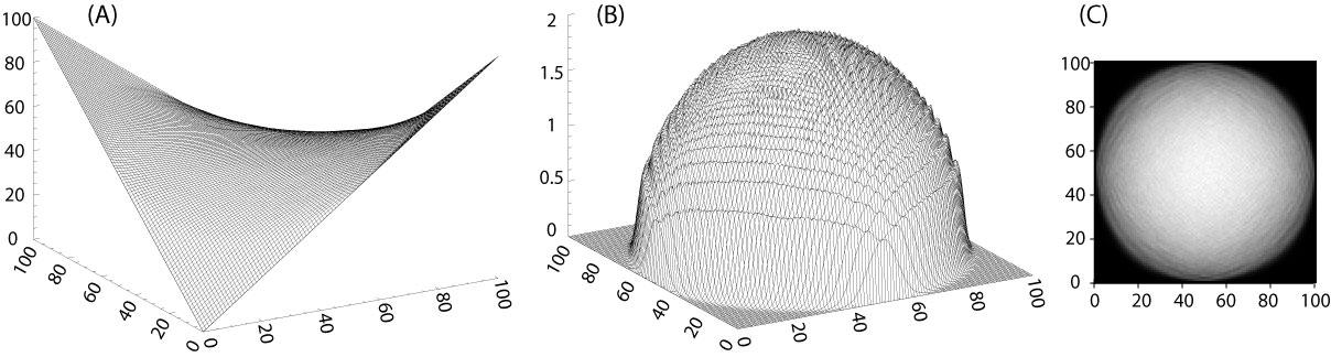
Figure 6: (A): The mean sphere stack surface in an $L=100$ tetrahedron. The surface is obtained by averaging over $10^{9}$ stacks at equilibrium. A typical surface at equilibrium is shown in Fig. 4F of the main text. (B): The corresponding probability of basic flips measured from $10^{9}$ step simulation. The probability distribution appears to be a hemisphere. (C): The flipping probability in (B) represented by brightness. The bright non-frozen region is circular, which agrees with the arctic circle theorem Jockush98 .

Combining the above results, $D(2n)\simeq\sum_{i=1}^{N_{n}}(2n-1)!!\prod_{j=0}^{n-1}k_{ij}\simeq(2n-1)!!N_{n}\bar{k}^{n}$, which becomes exact at the infinite-sized limit. Since $D(2)=N_{n}\bar{k}=N_{n}\sigma^{2}$, the $2n$th moment of the eigenvalue distribution $M(2n)=D(2n)/N_{n}=(2n-1)!!\sigma^{2n}$ is identical to the $2n$th moment of a Gaussian distribution. Therefore, spectral densities of phase-space networks are Gaussian at the infinite-sized limit. In fact, Fig. 3 in the main text shows that spectral densities are already very close to the Gaussian distribution when systems are small ($\sim 10^{3}$ nodes).

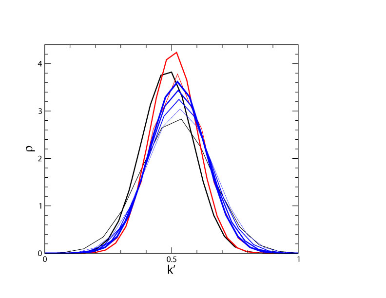
Figure 7: The probability distribution of normalized connectivity, $k^{\prime}=k/k_{max}$, where the maximum connectivity is $k_{max}\propto N_{spin}\propto L^{2}$. This figure is normalized from Fig. 2 in the main text. Black curves: cube stacks in $L=4$ (thick curve) and $L=3$ (thin) boxes. Red curves: sphere stacks in $L=7$ (thick) and $L=6$ (thin) tetrahedra. Blue curves: 2D square stacks (i.e., 2D sphere stack as shown in Fig. 15A) with $L=11,10,9,8$ (thicker curves for larger $L$). The peaks are in the middle bin at 0.5, i.e., $k=k_{max}/2$ has the highest number of stack configurations. In the infinite-sized limit, the normalized distributions will be asymptotic to a specific functional form. For a histogram of Fig. 2 in the main text before the normalization, the peak height, $H$, increases exponentially with the system size, while the heights at $k_{max}$ are always 1 or 2 (for example, see Fig. 8). Thus, their ratio $2/H\to 0$ in infinitely large systems. This indicates that the asymptotic distribution is indeed a Dirac delta function as described in ref. Destainville98 .

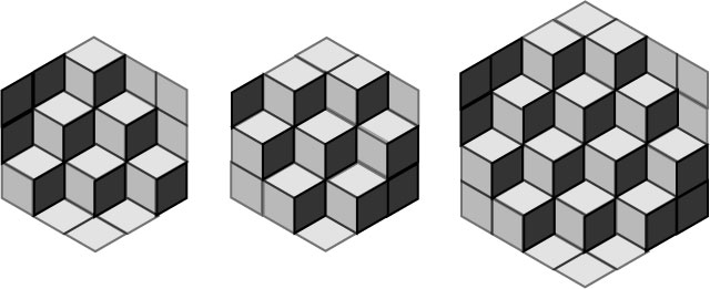
Figure 8: The two highest connectivity ($k=13$) states in $L=3$ (odd) cube stacks and the highest connectivity ($k=24$) state in $L=4$ cube stacks.

XII Appendix B: Dynamics in phase-space networks with weighted edges

In the main text, we show that trajectories spend equal amounts of time at every node on average. This can be easily generalized to networks with weighted edges, which, for example, can represent different potential barriers at finite temperatures. We replace an edge, $i$, with weight $w_{i}$ with $w_{i}$ equivalent edges. By applying such replacement to all edges, we get a new network with all equally weighted edges. The new connectivity for node $i$ is $k_{i}^{w}=\sum_{j=1}^{N_{node}}w_{ij}$. For the same reason as shown in the main text, the mean staying time at node $i$ is $\propto 1/k_{i}^{w}$. The visiting probability is $\propto k_{i}^{w}$ by generalizing the theorem in ref.Noh04 to weighted networks Wu07 . In fact, the proof in ref.Noh04 can be directly applied to weighted networks. For a weighted network, the connectivity matrix, $A_{ij}=w_{ij}$, where $w_{ij}$ is the weight of the edge between nodes $i$ and $j$. The weighted connectivity is $k_{i}^{w}=\sum_{j}A_{ij}$. The transition probability from node $i$ to node $j$ is $A_{ij}/k_{i}^{w}$. Suppose a walker starts at node $i$ at time $t=0$. Then, the master equation for the probability, $P_{ij}$, to find the walker at node $j$ at time $t$ is given by Noh04 :

$$P_{i\to j}(t)=\sum_{j_{t-1}}\frac{A_{j_{t-1}j}}{k^{w}_{j_{t-1}}}P_{i,j_{t-1}}(t-1).$$ (3)

The transition probability, $P_{ij}(t)$, from node $i$ to node $j$ in $t$ steps can be explicitly expressed by iterating Eq. 3,

$$P_{i\to j}(t)=\sum_{j_{1},\cdots,j_{t-1}}\frac{A_{ij_{1}}}{k^{w}_{i}}\frac{A_{j_{1}j_{2}}}{k^{w}_{j_{1}}}\cdots\frac{A_{j_{t-1}j}}{k^{w}_{j_{t-1}}}.$$ (4)

By comparing the expressions of $P_{i\to j}(t)$ and $P_{j\to i}(t)$, we get

$$k_{i}^{w}P_{i\to j}(t)=k_{j}^{w}P_{j\to i}(t).$$ (5)

We define the stationary probability, $P_{i}^{\infty}$, as $t\to\infty$. Eq. 5 implies that $k_{i}P_{j}^{\infty}=k_{j}P_{i}^{\infty}$ and, consequently, we obtain

$$P_{i}^{\infty}=\frac{k_{i}^{w}}{\sum_{i}k_{i}^{w}}=\frac{\sum_{i}A_{ij}}{\sum_{i,j}A_{i,j}}.$$ (6)

A random walker visits node $i$ at frequency $P_{i}^{\infty}\sim k_{i}^{w}$ and stays at node $i$ for the time period $\sim 1/k_{i}^{w}$ on average. Thus the walker spends the same amount of time at each node.

XIII Appendix C: Square ice and sphere stacks

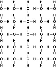
Figure 9: (A) Square ice with a domain wall boundary condition. Water molecules are frozen into a square lattice. This configuration corresponds to Figs. 4A, D, E in the main text.

Figure 9 shows a $5\times 5$ square ice with the domain wall boundary condition (DWB) corresponding to Figs. 4A, D, E. in the main text. Figure 10 shows $6\times 6$ spin ices with DWB and their corresponding FCC sphere stacks in an $L=5$ tetrahedron. Flipping all counterclockwise four-spin loops to clockwise corresponds to adding one layer of spheres. The tetrahedron emerges from the maximum packing, i.e., the full state.

A square plaquette can flip only when its four neighbors have the same height, which indicates that one building block in the 3D stack should be supported by four building blocks underneath. Thus, the stack can also be viewed as a body-centered cubic (BCC) lattice Beijeren77 . Both FCC and BCC stacking have the same combinatoric properties since they are only different by a stretch (see a 2D analogy in Fig. 15A). FCC is better than BCC because (1) FCC can be viewed as close-packed spheres in simple container shapes; (2) FCC has simple polyhedra stacking under gravity. The Wigner-Seitz cell of an FCC lattice is a rhombic dodecahedron, which is supported by four rhombic dodecahedra underneath, while the Wigner-Seitz cell of a BCC lattice can be supported by one block underneath since it has a flat square on the top.

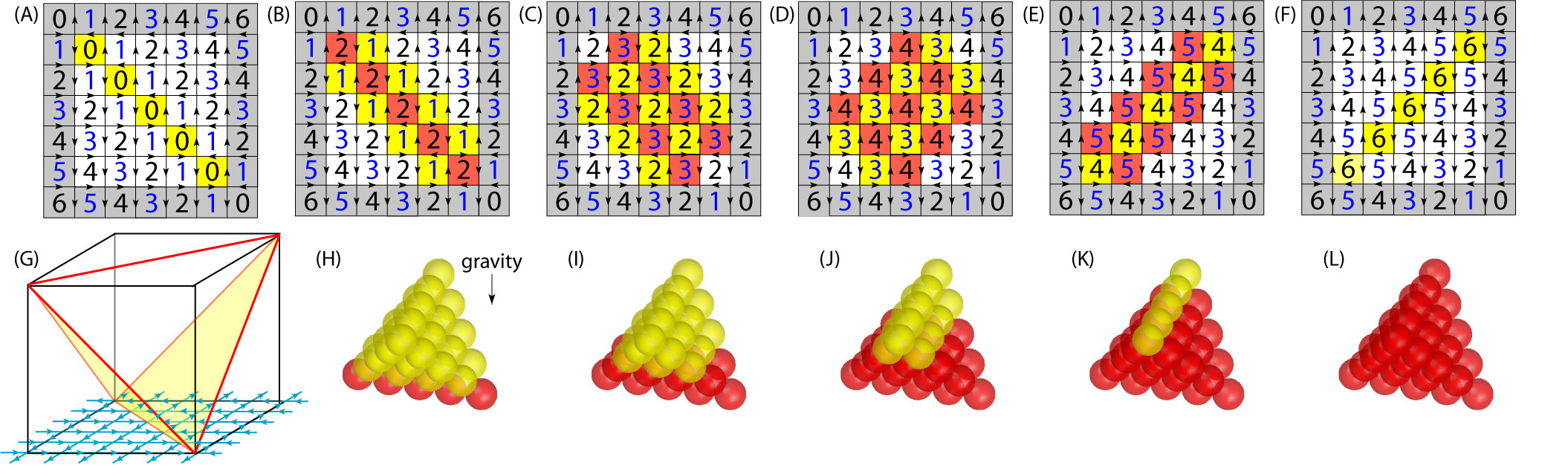
Figure 10: The one-to-one mapping between square ice and sphere stacks. (A-F): $6\times 6$ square ices. The domain wall boundary condition is labeled in grey. The height of each square plaquette is labeled with a number ranging from 0 to 6. The upper left corner is defined as zero height. Other heights are generated by the height rule in Fig. 5B in the main text. (A): the vacant state with the lowest possible heights. Heights in (F) define a container consisting of two yellow triangles shown in (G). Counterclockwise four-spin loops are labeled in yellow. Flipping all of them in (A) leads to the configuration in (B). Clockwise four-spin loops are labeled in red. Flipping the yellow plaquettes results a series of states shown in (C, D, E, and F). (F) has the highest possible heights without yellow plaquettes. These heights define a lid, which is an upside-down container in (G). All legal square ice configurations can be generated by flipping yellow plaquettes from the vacant state or, reversely, by flipping red plaquettes from the full state. A plaquette can be flipped only when its four neighbour plaquettes have the same height. The height of each plaquette is the physical height of the corresponding spheres on the top surface of the stack. Each basic flip can be viewed as adding or removing a sphere. (H-L): the red sphere stacks corresponding to (B-F). The yellow spheres are vacant sites.

XIV Appendix D: Boundary effects

We use the ‘alternating boundary condition’ shown in 11A, B to elucidate the lid-container duality. Given a boundary condition, the minimum (or maximum) possible heights can be directly written out, for example see Figs. 11A, B. These heights define the lid and the container. The lid and the container have different shapes. The container contains multiple height minima and the lid contains one height maximum (see the colored squares in Figs. 11A, B). They form an interesting pair of dual surfaces: using one as the container, the other will emerge as the surface of the highest ‘sand pile’ of small spheres. In fact, given a fixed boundary condition, the container and the lid are dual surfaces because, if we reverse the height rule in Fig.4(B), the container and the lid switch roles. Packing spheres in the container is equivalent to packing buoyant spheres in the corresponding lid. The height difference between a lid and container is a pyramid; for example, see Figs. 11 and 13.

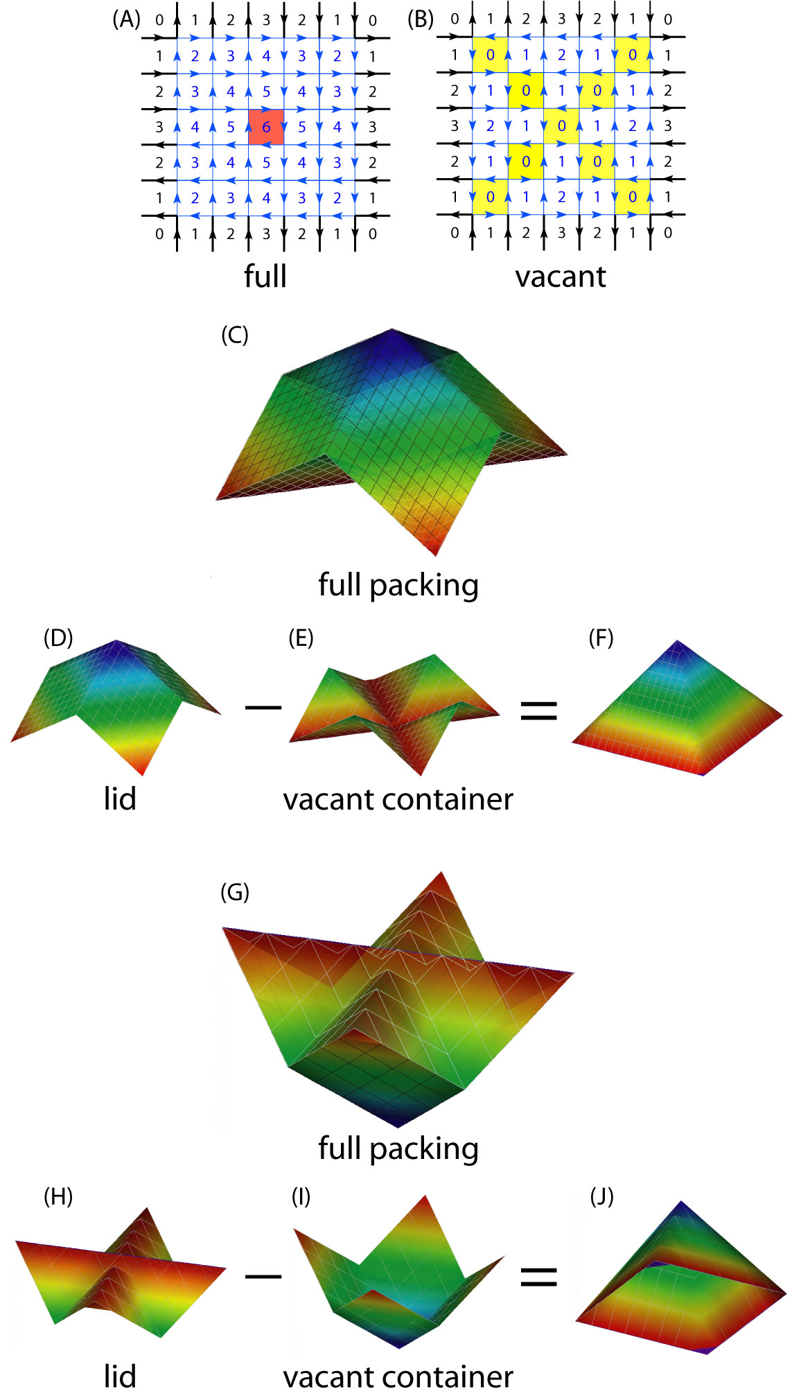
Figure 11: $6\times 6$ square ice with the ‘alternating boundary condition’. (A): The maximum possible heights, i.e., the lid, contains one clockwise basic flip labeled in red. (B): the minimum possible height, i.e., the container, contains multiple counterclockwise basic flips labeled in yellow. (C): The 3D shape of a full stack, including a lid (D) and a container (E). (F): The height difference between the lid and the container is a pyramid. (G-J): Upside-down geometries of (C-F). The lid (H) emerges from the maximum packing in the container (I), which is the upside-down version of (D).

Some boundary conditions do not exhibit the arctic circle phenomenon shown in Fig. 6. Their disordered region may not have a circular shape or may not even have a frozen area Eloranta99 . The container shape provides an intuitive understanding about how boundaries affect the disordered region. In a tetrahedron, the largest horizontal cross section is a square in the middle height that is circumscribed by the disordered region. In an octahedron, the largest horizontal cross section is the total square ice area so that there is no frozen region under the boundary condition shown in Fig. 4G of the main text. This is confirmed by our simulation. Other boundary conditions may lead to the non-circular disordered region. For example, the flower shape observed in ref. Eloranta99 (see Fig. 12B) is a direct consequence of the container shown in Fig. 12A.

The ensemble average over random stacks results a mean surface shown in Fig. S1A. At the infinite-sized limit, dominate states are close to this mean surface Destainville98 , i.e., the typical surface in Fig. 4F approaches the mean surface in Fig. S1A when $L\to\infty$. In the space of the stack surface, the distribution peaks around this maximum possible surface and becomes more and more like a Dirac delta distribution when approaching the infinite-sized limit Destainville98 . The local gradient of the surface determines the density of the basic flips, i.e., the density of configurational entropy $s_{0}$ Destainville98 . In Fig. S1A , the $s_{0}$ is zero in the frozen areas and continuously varies to reach its maximum value near the center of the square ice, with a non-zero gradient everywhere except near the center Destainville98 . Consequently, the infinitely large limit of the DWB cannot be called the thermodynamic limit due to the lack of homogeneity. In contrast, the boundary condition in Fig. 4G has the thermodynamic limit since the limiting surface in the octahedron is flat everywhere. The flat surface has the maximum possible $s_{0}$ (for example, see Fig. S3) so that its spatial averaged, $\bar{s}_{0}$, is as high as that of the free boundary condition. The boundary condition in Fig. 4G is a subset of the periodic boundary condition, so that the periodic boundary condition has the same $\bar{s}_{0}$ as the free boundary condition at the infinite-sized limit. This explains why the $\bar{s}_{0}$ calculated from the periodic boundary condition Nagle66 agrees so well with the experimental results on water ice obtained under the free boundary condition Giauque33 . When the height difference of a fixed boundary is comparable to $L$, the limiting surface is not flat and $\bar{s}_{0}$ is smaller. For example, the zero-point entropy of $L\times L$ square ice in the infinite-sized limit under DWB is $\bar{s}_{0}=k_{B}L^{2}\ln{N_{n}}=k_{B}\ln(\sqrt{27/16})$ Elkies92 based on Eq. 2 in the main text, which is smaller than $k_{B}L^{2}\ln(\sqrt{64/27})$ under the periodic boundary condition Lieb67 . For cube stacks, $\bar{s}_{0}=k_{B}\ln(\sqrt{27/16})$ under the hexagonal boundary condition based on Eq. 1 in the main text, which is smaller than $0.323k_{B}$ under the periodic boundary condition Wannier50 .

The typical stack configuration in a tetrahedron or octahedron is $\sim$ 50% filled because the lid and the container have the same shape. When they have different shapes, a typical stack configuration may not be $\sim$ 50% filled. Figure 12A is the averaged surface in an $L=100$ container. The total volume has $L(L^{2}-1)/6$ spheres, and $\sim$42% of the volume is filled with spheres on average. Note that the largest horizontal cross-section is at $h=\sqrt{2}/3$ with a corresponding filled fraction of 4/9.

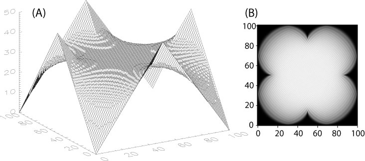
Figure 12: (A): The ensemble-averaged height surface for $L=100$ square ice with alternating boundary condition shown in Fig. 11A, B. The heights are rounded off to integers to show equal-height contours. The container shape is shown in Fig. 11E. (B): The flipping probability represented by the brightness.

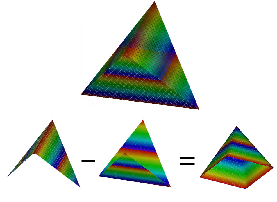
Figure 13: The lid, container and their height difference of a tetrahedron.

XV Appendix E: square ice with periodic boundary condition

Here, we use the $2\times 3$ square ices to illustrate that periodic boundary conditions result in disconnected phase-space networks. Figure 14 shows the 44 configurations of the $2\times 3$ square ice wrapped on a toroid. Note that this periodic boundary condition is for spins, not for heights. The upper left corner is defined as zero height. The 12 configurations in Fig. 14A are connected by basic flips and form a 12-node cluster as shown in Fig. 14D. The other 12 configurations in Fig. 14B form another 12-node cluster in Fig. 14D. The height difference between the top corners and bottom corners is +1 in Fig. 14A and -1 in Fig. 14B. Note that the four corners are essentially the same plaquette on the toroid, so they must be either all inside or all outside of a loop, such as the one shown in Fig. 14E. Consequently, the height difference between the corners cannot be changed by flipping a closed spin loop. Therefore, the nodes in Fig. 14A and B form two disconnected clusters. The 20 isolated nodes in Fig. 14D correspond to the 20 configurations in Fig. 14C, which contain no basic flips.

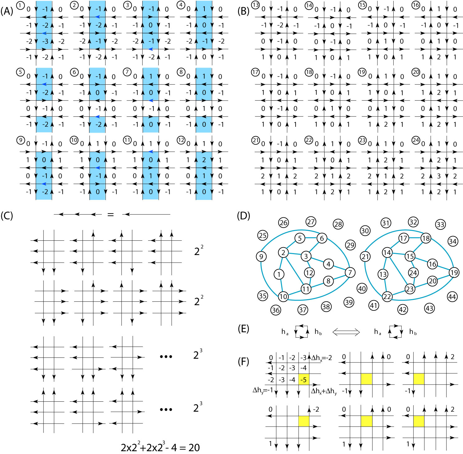
Figure 14: Configurations and the phase-space network of $2\times 3$ square ice wrapped on a toroid, i.e., with the periodic boundary condition. (A): Configurations 1 to 12. The upper left plaquette is defined as zero height and other heights are derived from it by using the height rule in Fig. 4B in the main text. (B): Configurations 13 to 24. (C): 20 configurations that contain no basic flip. They are categorized into four types: all horizontal spins are (1) leftwards; (2) rightwards; all vertical spins are (3) upwards; (4) downwards. Four configurations are double counted, so the total number of configurations is $2\times 2^{2}+2\times 2^{3}-4$. (D): The phase-space network. Two nodes are connected if they are different by one basic flip (i.e., the flip of a four-spin loop). (E): The flip of a spin loop does not change the height difference, $h_{a}-h_{b}$ if $h_{a}$ and $h_{b}$ are both inside or outside the loop. (F): $m\times n$ square ice ($m=3$, $n=4$) with periodic boundary conditions. There are $(m-1)\times(n-1)=6$ types of different $(\Delta h_{x},\Delta h_{y})$. Configurations with the same $(\Delta h_{x},\Delta h_{y})$ form one cluster by adding/removing spheres in the corresponding container, while configurations with different $(\Delta h_{x},\Delta h_{y})$ are disconnected because zero energy flips cannot change the height mismatches. Each state has a unique lowest height plaquette labeled in yellow.

We generalize the above results to the $m\times n$ periodic lattice and prove that it has $(m-1)\times(n-1)$ non-trivial clusters and $2^{n+1}+2^{m+1}-4$ isolated nodes. Unlike fixed boundary conditions, after walking along a closed loop in the $x$ or $y$ direction on a toroid and coming back to the original plaquette, the height may change. Such height differences, $\Delta h_{x}$ and $\Delta h_{y}$, uniquely characterize each disconnected subnetwork. Consider an arbitrary plaquette on a toroid. We unwrap the lattice onto a plane so that this plaquette is at the upper left corner with the height defined as 0, e.g., see Fig. 14F. As shown in Fig. 14E, any zero energy flip of a spin loop cannot change the height differences between the four corners since they are essentially the same plaquette on the toroid. Consequently, configurations with different $\Delta h_{x}$ or $\Delta h_{y}$ cannot be connected by basic flips. On the other hand, if configurations have the same $\Delta h_{x}$ and $\Delta h_{y}$, they must be connected because they have essentially the same fixed boundary condition after being unwrapped onto a plane (see Fig. 14F). Here, we use the fact that all legal configurations at a fixed boundary condition are connected by basic flips Eloranta99 . Since they are connected, we can choose the configuration whose bulk spins are along the boundary spins to represent each subnetwork (see examples in Figs. 14C, F). Next, we consider the number of representative configurations, i.e., the number of subnetworks. If a representative configuration has no basic flips, all of its horizontal spins or vertical spins have to be along the same direction as shown in Fig. 14C. The ‘energy barriers’ between these states are large for large systems because $m$ or $n$ spins need to flipped simultaneously in order to change from one state to another without breaking the ice rule. If all horizontal spins are leftwards (or rightwards), there are $2^{m}$ configurations for vertical spins (see Fig. 14C). If all vertical spins are upwards (or downwards), there are $2^{n}$ configurations for horizontal spins. In total, the four configurations are double counted so that there are $2^{n+1}+2^{m+1}-4$ isolated nodes, i.e., configurations without basic flips. Next, we consider nontrivial clusters with multiple nodes. The corner height difference, $\Delta h_{x}$, has $m-1$ possible values, and $\Delta h_{y}$ has $n-1$ possible values (see Fig. 14F), so that there are $(m-1)\times(n-1)$ nontrivial subnetworks in total. The representative configurations of the six subnetworks shown in Fig. 14F are chosen to have the lowest possible heights, i.e., vacant containers for sphere stacking. Each configuration is characterized by one basic flip labeled as yellow squares, i.e., the lowest point of the vacant container. Apparently, there are $(m-1)\times(n-1)$ positions for a yellow square, i.e., $(m-1)\times(n-1)$ subnetworks. This result confirms that the zero-point entropy $\bar{s}_{0}$ of the whole network is the same as that of the largest subnetwork under the constant-height boundary condition (see section IV) because $(m-1)\times(n-1)$ is logarithmically small compared with the total number of configuration $\sim e^{N_{spin}}\sim e^{m\cdot n}$.

Next, we show that the smallest nontrivial cluster has $\frac{(m+n-1)!}{(n-1)!(m-1)!}$ nodes. In Fig. 14F, the two middle configurations represent 132-node subnetworks and the other four configurations represent 60-node subnetworks. When the yellow square is at the corner, the height function indicates that the container shape is a tilted 2D container rather than a 3D container. Thus, the number of spheres packing in such a container is much smaller than that in 3D containers whose lowest point (the yellow plaquette) is not at the corner. To count the number of states in a tilted 2D container, we first consider the simple case in Fig. 14A. Configuration 1 in Fig. 14A is the representative state with the lowest height of -3. Configurations 1 to 4 in Fig. 14A have the same boundary spins so that we can view them as the 2D sphere stacks in the same $1\times 3$-sized 2D rectangle. Such a blue $1\times 3$ container has three possible positions relative to the zero height plaquette (see configurations 1, 5 and 9 in Fig. 14A). In total the subnetwork has $3\times 4=12$ nodes. It is easy to generalize this counting to $m\times n$ square ice on a toroid. There are $m$ possible positions for the $m\times(n-1)$-sized rectangle. With 2D sphere stacking in an $a\times b$ container, there are $C_{a+b}^{a}=(a+b)!/(a!b!)$ configurations (see Fig. 15 and its caption). Consequently, there are $mC_{m+n-1}^{m}=\frac{(m+n-1)!}{(n-1)!(m-1)!}$ nodes in the smallest nontrivial subnetworks. We confirm the above results numerically. Our numerical results also confirm the number sequence A054759 in ref.sequence for the $n\times n$ square ice under periodic boundary conditions.

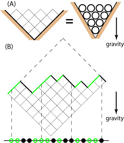
Figure 15: (A): 2D circle stacking is combinatorically equivalent to 2D square stacking because each circle or square is supported by two circles underneath in a gravity field. (B): Mapping a 2D stack of squares in an $a\times b=7\times 9$ container to a chain of $a$ solid particles and $b$ holes Okounkov03 . The dynamics, i.e., the diffusion of particles, is described as a symmetric simple exclusion process (SSEP). The number of 2D stack configurations in a container is $C_{a+b}^{a}=(a+b)!/(a!b!)$, i.e., the number of ways to put $a$ particles onto $a+b$ sites.

References

- (1) Albert, R. & Barabási, A.-L. Statistical mechanics of complex networks. Rev. Mod. Phys. 74, 47-97 (2002).
- (2) Newman, M. E. J. The structure and function of complex networks. SIAM Rev. 45, 167-256 (2003).
- (3) Costa, L. D. F., Rodrigues, F. A., Travieso, G. & Boas, P. R. Characterization of complex networks: a survey of measurements. Adv. Phys. 56, 167-242 (2007).
- (4) Moessner, R. & Ramirez, A.R. Geometrical frustration. Phys. Today 59, 24-26 (2006).
- (5) Pauling, L. The structure and entropy of ice and of other crystals with some randomness of atomic arrangement. J. Am. Chem. Soc. 57, 2680-2684 (1935).
- (6) Bramwell, S. T. & Gingras, M. J. P. Spin ice state in frustrated magnetic pyrochlore materials. Science 294, 1495-1501 (2001).
- (7) Wang R. F. et al., Artificial ‘spin ice’ in a geometrically frustrated lattice of nanoscale ferromagnetic islands. Nature 439, 303-306 (2006).
- (8) Han Y. et al., Geometric frustration in buckled colloidal monolayers. Nature 456, 898-903 (2008).
- (9) Wannier, G. H. Antiferromagnetism. the triangular Ising net. Phys. Rev. 79, 357-364 (1950); erratum Phys. Rev. B 7, 5017 (1973).
- (10) Blöte, H. W. J. & Nienhuis, B. Fully packed loop model on the honeycomb lattice. Phys. Rev. Lett. 72, 1372-1375 (1994).
- (11) Andrews, G. E. & Eriksson, K. Integer Partitions (Cambridge University Press, 2004).
- (12) Andrews, G. E. Percy Alexander MacMahon: Collected Papers, Vol. 2 (The MIT Press, Cambridge, 1986).
- (13) http://www.research.att.com/njas/sequences/
- (14) Watts, D. J. & Strogatz, S. H. Collective dynamics of ‘small-world’ networks. Nature 393, 440-442 (1998).
- (15) Barabási, A.-L. & Albert, R. Emergence of scaling in random networks. Science 286, 509-512 (1999).
- (16) Farkas, I. J., Derényi, I., Barabási, A.-L. & Vicsek, T. Spectra of “real-world” graphs: beyond the semicircle law. Phys. Rev. E 64, 026704 (2001).
- (17) de Aguiar, M. A. M. & Bar-Yam, Y. Spectral analysis and the dynamic response of complex networks. Phys. Rev. E 71, 016106 (2005).
- (18) Newman, M. E. J. Modularity and community structure in networks. Proc. Nat. Acad. Sci. 103, 8577-8582 (2006).
- (19) Patrascioiu A. The ergodic hypothesis. Los Alamos Science, 15, 263 (1987).
- (20) Noh, J. & Rieger, H. Random walks on complex networks. Phys. Rev. Lett. 92, 118701 (2004).
- (21) Cohen, E. G. D. Boltzmann and Einstein: statistics and dynamics - an unsolved problem. Pramana 64, 635-643 (2007).
- (22) Bressoud, D. M. Proofs and Confirmations: The Story of the Alternating-Sign Matrix Conjecture (Cambridge University Press, 1999).
- (23) Propp, J. G. The many faces of alternating-sign matrices. Discrete Math. Theoret. Comput. Sci. Proc. AA, 43-58 (2001).
- (24) Eloranta, K. Diamond ice. J. Stat. Phys. 96, 1091-1109 (1999).
- (25) van Beijeren, H. Exactly solvable model for the roughening transition of a crystal surface. Phys. Rev. Lett. 38, 993-996 (1977).
- (26) Millane, R. P. & Blakeley, N. D. Boundary conditions and variable ground state entropy for the antiferromagnetic Ising model on a triangular lattice. Phys. Rev. E 70, (2004).
- (27) Destainville, N. Entropy and boundary conditions in random rhombus tilings. J. Phys. A: Math. Gen. 31, 6123-6139 (1998).
- (28) Jockush, W., Propp, J. & Shor, P. Random domino tilings and the arctic circle theorem. Preprint at http://arxiv.org/abs/math/9801068 (1998).
- (29) Lieb, E. H. Exact Solution of the problem of the entropy of two-dimensional ice. Phys. Rev. 162, 162-172 (1967).
- (30) Moessner, R. & Chalker, J. T. Low-temperature properties of classical geometrically frustrated antiferromagnets. Phys. Rev. B 58, 12049-12062 (1998).
- (31) Lee S. H. et al., Emergent excitations in a geometrically frustrated magnet. Nature 418, 856-858 (2002).
- (32) Blunt M. O. et al. Random tiling and topological defects in a two-dimensional molecular network. Science 322, 1077-1081 (2008).
- (33) Moore, C. & Newman, M. E. J. Height representation, critical exponents, and ergodicity in the four-state triangular Potts antiferromagnet. J. Stat. Phys. 99, 629-660 (2000).
- (34) Song, C., Havlin, S. & Makse, H. A. Self-similarity of complex networks. Nature 433, 392-395 (2005).
- (35) Gfeller, D. & De Los Rios, P. Spectral coarse graining of complex networks. Phys. Rev. Lett. 99, 038701 (2007).
- (36) Cho, A. A Fresh take on disorder, or disorderly science? Science 297, 1268-1269 (2002).
- (37) Gell-Mann, M. & Tsallis, C. Nonextensive Entropy - Interdisciplinary Applications, (Oxford University Press, New York, 2004).
- (38) Baxter, R. J. Exactly Solved Models in Statistical Mechanics (Academic Press, London, 1982).
- (39) Okounkov, A., Reshetikhin, N. & Vafa, C. Quantum Calabi-Yau and classical crystals. Preprint at http://arxiv.org/abs/hep-th/0309208 (2003).
- (40) Kenyon, R. & Okounkov, A. Limit shapes and the complex burgers equation. Preprint at http://arxiv.org/abs/math-ph/0507007 (2007).
- (41) Elkies, N., Kuperberg, G., Larsen, M. & Propp, J. Alternating-sign matrices and domino tilings. J. Algebraic Geom. 1, 111-132 (1992).
- (42) Wu, A.-C., Xu, X.-J., Wu, Z.-X. & Wang, Y.-H. Chin. Phys. Lett. 24, 577 (2007).
- (43) Nagle, J. F. J. Math. Phys. 7, 1484 (1966).
- (44) Giauque, W. F. & Ashley, M. F. Phys. Rev. 43, 81 (1933).
- (45) Okounkov, A. Preprint at http://arxiv.org/abs/math-ph/0309015 (2003).