Models of high redshift luminosity functions and galactic outflows: The dependence on halo mass function

Abstract

The form of the halo mass function is a basic ingredient in any semi-analytical galaxy formation model. We study the existing forms of the mass functions in the literature and compare their predictions for semi-analytical galaxy formation models. Two methods are used in the literature to compute the net formation rate of halos, one by simply taking the derivative of the halo mass function and the other using the prescription due to Sasaki (1994). For the historically used Press-Schechter (PS) mass function, we compare various model predictions, using these two methods. However, as the Sasaki formalism cannot be easily generalized for other mass functions, we use the derivative while comparing model predictions of different mass functions. We show that the reionization history and UV luminosity function of Lyman break galaxies (LBGs) predicted by the PS mass function differs from those using any other existing mass function, like Sheth-Tormen (ST) mass function. In particular the reionization efficiency of molecular cooled halos has to be substantially reduced when one uses the ST and other mass functions obtained from the simulation instead of the PS mass function. Using $\chi^{2}$-minimization, we find that the observed UV luminosity functions of LBGs at $3.0\leq z\leq 7.4$ are better reproduced by models using the ST mass function compared to models that use the PS mass function. On the other hand, the volume filling factor of the metals expelled from the galaxies through supernovae driven outflows differs very little between models with different mass functions. It depends on the way we treat merging outflows. We also show that the porosity weighted average quantities related to the outflow are not very sensitive to the differences in the halo mass function.

1 Introduction

The formation of galaxies and their influence on the physical state of the inter-galactic medium (IGM) is often studied using semi-analytical models of structure formation (for example 1991, 1993, 1994, 1999, 2000, 2001, 2001, 2005). Such studies will allow one to extensively explore the unknown parameter space related to physical conditions in a high redshift galaxy and its star formation, with limited computational resources. Semi-analytical models together with available observations can be used to understand the evolution of our universe while putting tight constraints on various physical processes associated with the high redshift universe. In Samui et al. (2007, 2008) (hereafter Paper I and Paper II) we used semi-analytical models to predict the ionization history of the universe, the high redshift ($z\geq 3$) UV luminosity functions of LBGs and also the global effect of galactic outflows.

In any semi-analytical galaxy formation model, one needs to assume some form of the halo mass function giving the number density of dark matter halos as a function of mass and redshift. The first halo mass function in an analytical form was given by Press & Schechter (1974). The Press-Schechter (PS) mass function has been widely employed in semi-analytical models of galaxy formation and in understanding the high redshift universe. It is important to note that one needs not just the dark halo mass function at any redshift, but also their formation rate and survival probability. For the PS mass function, Sasaki (1994) proposed a method to find the formation rate of halos and their survival probability at later epochs. Note that one can also find this rate through N-body simulations, or by constructing a large number of merger trees. However, it turns out that we need to resolve halo masses over a wide dynamic range from $10^{7}M_{\odot}$ to $10^{12}M_{\odot}$, to model both the effect of outflows and the galactic luminosity function. One also needs to have a large enough number of halos in the simulation or a large number of realizations of the merger trees, to obtain good statistics of the range of galaxy properties. Therefore, to have a preliminary look at this challenging problem, in Paper I and  II, we focused on analytical methods. In particular we used the PS mass function and the Sasaki formalism, to predict the ionization history of the universe, the high redshift ($z\geq 3$) UV luminosity functions and also the global effect of galactic outflows.

In Paper I, we concluded that the observed redshift evolution of the luminosity function of Lyman break galaxies (LBGs) at $z\geq 3$ requires evolution in physical properties that govern the star formation activity on top of the evolution in the number density of dark matter halos coming from the structure formation model. We found that the required amount of redshift evolution in the star formation activities depends on the redshift evolution of the number density of dark matter halos and hence on the assumed form of the halo mass function.

In Paper II, we showed that galactic scale outflows originating predominantly from small mass halos with mass $10^{7}-10^{9}~{}M_{\odot}$ can pollute 60% of the IGM with metals at $z\sim 3$ with a metallicity floor of $10^{-3}Z_{\odot}$. Inclusion of star formation in even smaller mass halos which cool due to the presence of H₂ or HD molecules, helps more in spreading the metals. This is because they are more abundant and hence their mean separation is smaller. In these models, even at $z=8$, more than 60% of IGM is being polluted with metals. These conclusions may crucially depend on the choice of the adopted form of the mass function.

It is known that the PS mass function does not provide a good fit to the number density of dark matter halos determined from recent high resolution simulations of galaxy formation. From such simulations a number of different fitting formulae for the halo mass function have been suggested (see for example Sheth & Tormen 1999; Jenkins et al. 2001; Reed et al. 2003, 2007 and Warren et al. 2006). Note that there is no direct way to scale the results obtained by assuming the PS mass function to results which would arise from these other mass functions. Therefore it is important to revisit various issues discussed in Paper I and II considering the mass functions determined from the simulations. This forms the basic motivation of this paper. We will mainly concentrate, as in Paper I and II, on high redshift (i.e. $z\geq 3$) UV luminosity function of Lyman break galaxies (LBGs) and the effect of galactic outflows on the IGM adopting a self consistent reionization history.

Note that the Sasaki formalism, used in Paper I and II, is not easily generalisable to other mass functions (Ripamonti, 2007 and also see discussion in section 2). An alternative is to simply take the derivative of the mass function under the assumption that it is sufficiently close to the net formation rate of objects in the mass range that is of interest to the semi-analytic models. This approach is widely used in several semi-analytical models in the literature (for example Haehnelt & Rees 1993, Scannapieco 2005). The derivative includes not only the formation rate of halos, but also their destruction rate at the same redshift. Therefore it is not guaranteed to be positive definite. This is the disadvantage of using the derivative of the mass function. Nevertheless, in the range of halo masses that we will be interested in at different redshifts, we will see that the derivative of the mass function is indeed positive definite. Therefore, for other mass functions consider in this work, we simply use its derivative to model the net formation rate of dark matter halos. We will also compare results obtained using the derivative as an alternative to the Sasaki formalism for the PS mass function.

The paper is organized as follows. In section 2 we review different proposals for the halo mass function that we wish to study and also compare the net formation rate of collapsed halos predicted by these mass functions. The star formation and reionization models are described in section 3. In section 4 we show the effect of the halo mass function on the predicted UV luminosity functions of high redshift LBGs. In particular, we use the $\chi^{2}$-minimization technique to discriminate between models using different mass functions. The feedback of galactic outflows on the IGM is discussed in section 5. Finally section 6 gives our conclusions. In this work we use the cosmological parameters consistent with the recent WMAP 5th year data release i.e. $\Omega=1$, $\Omega_{m}=0.26$, $\Omega_{\Lambda}=0.74$, $\Omega_{b}=0.044$, $h=0.72$, $\sigma_{8}=0.80$ and $n_{s}=0.96$ (Dunkley et al. 2008). Also we use a Salpeter stellar initial mass function (IMF) in the mass range $1-100~{}M_{\odot}$ unless otherwise mentioned.

2 Comparing halo mass functions

The halo mass function is defined to be the number density of collapsed dark matter halos in the mass range $M$ and $M+{\rm d}M$ at a given redshift $z$. The differential halo mass function is defined as

$$\frac{{\rm d}N}{{\rm d}M}=\frac{\rho_{0}}{M}\frac{{\rm d}\ln\sigma^{-1}}{{\rm d}M}f(\sigma)$$ (1)

where $\rho_{0}$ is the average density of the universe at that redshift. The rms density fluctuations, $\sigma$, of the smooth density field with a top-hat window function is defined as

$$\sigma^{2}=D^{2}(z)\sigma_{0}^{2}=D^{2}(z)\frac{1}{2\pi^{2}}\int\limits_{0}^{\infty}k^{2}P(k)W^{2}(k,M){\rm d}k$$ (2)

where, $P(k)$ is the linear power spectrum of the density fluctuations at $z=0$, $W(k,M)$ is the Fourier transform of the real-space top-hat filter, and $D(z)$ is the growth factor of linear perturbations normalized to unity at $z=0$ (Peebles 1993, Padmanabhan 2002). The idea of representing the mass function in the form of Eq. 1 is that different analytical forms of the halo mass function can be represented with different forms of the function $f(\sigma)$ in that equation. For example, $f(\sigma)$ for the PS mass function is given by

$$f_{PS}(\sigma)=\sqrt{\frac{2}{\pi}}\frac{\delta_{c}}{\sigma}\exp{\left(-\frac{\delta_{c}^{2}}{2\sigma^{2}}\right)}$$ (3)

where $\delta_{c}$ is the critical over density for collapse, usually taken to be equal to $1.686$. The simple form of PS mass function has been widely used in the semi-analytical models of galaxy formation (Chiu & Ostriker 2000, Barkana & Loeb 2001, Nagamine et al 2006).

The deviation of the PS mass function from numerical simulations was pointed out by Sheth & Tormen (1999). The discrepancy is larger for high mass rare objects, the PS mass function always predicting a smaller number of rare objects compared to numerical simulations. Sheth & Tormen (1999) proposed a modification of the PS mass function which provides a better fit to the numerical simulation data. The Sheth-Tormen (ST) mass function takes the following form:

$$f_{ST}(\sigma)=A\sqrt{\frac{2a}{\pi}}\left[1+\left(\frac{\sigma^{2}}{a\delta_{c}^{2}}\right)^{p}\right]\frac{\delta_{c}}{\sigma}\exp{\left(-\frac{a\delta_{c}^{2}}{2\sigma^{2}}\right)}.$$ (4)

Choosing $A=0.3222$, $a=0.707$ and $p=0.3$ in Eq. 4 provides a better fit to mass functions obtained from numerical simulations over a wide range of masses and redshifts compared to the PS formula. Note that, if we take $A=0.5$, $a=1.0$ and $p=0.0$ in Eq. 4 then the ST mass function reduces to the PS mass function.

Further, Jenkins et al. (2001) found deviation from the ST mass function in their simulations of the $\tau$CDM and $\Lambda$CDM cosmologies. They proposed another $f(\sigma)$ which fits better their own simulations over more than four orders of magnitude in mass, $\sim 3\times 10^{11}$ to $\sim 5\times 10^{15}~{}h^{-1}M_{\odot}$. This mass function, referred to here as Jenkins & White (JW) mass function is given by

$$f_{JW}=0.315\exp{\left[-|\ln\sigma^{-1}+0.61|^{3.8}\right]}.$$ (5)

Another study of $f(\sigma)$ was made by Reed et al.(2003). They used high-resolution $\Lambda$CDM numerical simulations to calculate $f(\sigma)$ of dark matter halos down to the scale of dwarf galaxies, back to a redshift of $15$. They showed that the ST mass function provides a good fit to their data except for redshift $10$ or higher where it over predicts halo numbers by more than $50\%$. In a later work, Reed et al. (2007) developed a new method for compensating the effects of finite simulation volume. This allowed them to find an approximation to the true ‘global’ mass function. They proposed another fitting formula given by

$$f_{R}(\sigma) = A\sqrt{\frac{2a}{\pi}}\left[1+\left(\frac{\sigma^{2}}{a\delta_{c}^{2}}\right)^{p}+0.6G_{1}+0.4G_{2}\right]\frac{\delta_{c}}{\sigma}$$ (6)

$$\exp{\left[-\frac{ca\delta_{c}^{2}}{2\sigma^{2}}-\frac{0.03}{(n_{eff}+3)^{2}}\left(\frac{\delta_{c}}{\sigma}\right)^{0.6}\right]}$$

where

$$G_{1} = \exp{\left[-\frac{[\ln\sigma^{-1}-0.4]^{2}}{2(0.6)^{2}}\right]}$$ (7)

$$G_{2} = \exp{\left[-\frac{[\ln\sigma^{-1}-0.75]^{2}}{2(0.2)^{2}}\right]}$$ (8)

and

$$\frac{n_{eff}+3}{6}=\frac{{\rm d}\log\sigma^{-1}}{{\rm d}\log M}$$ (9)

The values of constants which require to fit the numerical simulations are $c=1.08$, $ca=0.764$, and $A=0.3222$.

Meanwhile Warren et al. (2006) performed simulations where they corrected a systematic error in halo-mass determination by the friends-of-friends halo finder. They also measured the shape and quantified the uncertainty in the predicted theoretical mass function of dark matter halos in $\Lambda$CDM cosmology and showed that the canonical ST and JW forms of the mass function are inconsistent with the $\Lambda$CDM mass function at a $\sim 10\%$ level at intermediate masses, and $>30\%$ at the highest masses. They provided an analytical fit to $f(\sigma)$ given by

$$f_{W}(\sigma)=0.7234\left(\sigma^{-1.625}+0.2538\right)\exp{\left[-\frac{1.1982}{\sigma^{2}}\right]}.$$ (10)

Thus we have a set of halo mass functions which gives a better fit to the numerical simulations of galaxy formation compared to the classical PS formula. Here, we consider these set of $f(\sigma)$ to examine how sensitive the predictions of semi-analytical models are to the assumed form of the halo mass function.

We begin by comparing the net formation rate of dark matter halos for different halo mass functions described above. This is the most fundamental ingredient in any semi-analytical model of galaxy formation. In Paper I & II we used Sasaki formalism of the PS mass function to get the formation rate. Following the same steps for the ST mass function we obtain

$${\cal N}_{s}(M,z,z_{c}) = \frac{\rho_{0}}{M}\left(-\frac{1}{\sigma}\frac{{\rm d}\sigma}{{\rm d}M}\right)f_{ST}(\sigma)\left(\frac{1}{D(z_{c})}\frac{{\rm d}D(z_{c})}{{\rm d}z_{c}}\right)$$ (11)

$$\left[\frac{{\rm d}\ln f_{ST}(\sigma)}{{\rm d}\ln\sigma}+(1-2p)\right]\left[\frac{D(z_{c})}{D(z)}\right]^{1-2p}$$

where ${\cal N}_{s}(M,z,z_{c})$ is the formation rate of the dark matter halos collapsed at $z_{c}$ and survive till some observed redshift, $z\leq z_{c}$. The survival probability is given by $[{D(z_{c})}/{D(z)}]^{(1-2p)}$. Note that putting $A=0.5$, $a=1.0$ and $p=0$ in above equation gives back the Sasaki formalism of the PS mass function (see eq. 1 of Paper I). It is clear from the above equation that due to the presence of $-2p$ term, it is not guaranteed that the formation rate will always be positive. As formation rate being negative is unphysical the generalization of Sasaki formalism for the ST mass function is incorrect. Therefore, as mentioned in section 1, we rather model the net formation rate of collapsed dark matter halos, by taking the redshift derivative of the halo mass function, ${\cal N}(M,z_{c})={\rm d}^{2}N/{\rm d}M{\rm d}z_{c}$.

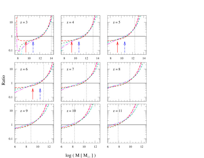
Figure 1: The net formation rate of dark matter halos, ${\cal N}$, for different halo mass functions at different redshifts. We compare the redshift derivative of different mass functions with the derivative of the PS mass function (shown by the solid line). We show the derivative of ST (long dashed, red), JW(dot long dashed, magenta), Warren (dot short dashed, cyan) and Reed (short dashed, dark green) mass functions. The vertical dashed line in each panel shows the mass of typical collapsing objects from $3\sigma$ fluctuations. The solid (red) and dashed (blue) arrows in redshift $3\leq z\leq 6$ indicate the halo masses correspond to circular velocities $v_{c}=35~{}$km s^-1 and $95~{}$km s^-1 respectively.

In Fig. 1 we show the ratio of the redshift derivatives for different halo mass functions to that obtained for the PS mass function. In panels with $3\leq z\leq 6$ we show three characteristics masses related to our star formation model at that redshift. The dotted vertical lines show the mass that collapsed from $3\sigma$ fluctuations at that redshift. In addition with solid (red) and dashed (blue) arrows we show the masses corresponding to halos with circular velocity $v_{c}=35~{}km~{}s^{-1}$ and $95~{}km~{}s^{-1}$ respectively. This is the mass range where radiative feedback from the metagalactic UV background becomes important (Thoul & Weinberg 1996, also see in Sec. 3). In this redshift range the process of reionization is believed to be already over (Fan et al. 2006) and hence the radiative feedback is well constrained in our model (indeed we will see in the next section that all our models predict redshift of reionization $z_{re}\geq 6$). We do not show these arrows for $z>6$ as the exact radiative feedback will depend on the history of reionization. Thus, for $z>6$ we only show the mass that collapsed from a $3\sigma$ fluctuations by dotted lines.

It is clear from the figure that for higher mass objects which are rare, the PS mass function always predicts a smaller net halo formation rate compared to any other mass function. For smaller mass objects the trend is opposite. This will lead to different slope in the luminosity function derived from different halo mass function. At $z\geq 6$ all the mass functions predict similar halo formation rate (within 10%) around the characteristic mass which corresponds to $3\sigma$ fluctuations. However, at the typical halo masses that will be detected as galaxies ($\geq 10^{10}{\rm M}_{\odot}$) PS underpredicts the net halo formation rate upto an order of magnitude.

For $z\lesssim 5$ the $3\sigma$ fluctuations are above $10^{12}~{}M_{\odot}$ and the predictions of other mass functions compared to that of PS mass function are upto an order of magnitude higher. However, in our modelling of star formation, we assume a sharp cut off in the star formation for halos of mass above $10^{12}~{}M_{\odot}$, attributed to the AGN feedback (see section 2 of Paper I). This reduces the difference in the prediction of our semi-analytical modelling of star formation arising due to different halo mass functions at these redshifts. Hence, for $z\lesssim 5$ all the mass functions predict a halo formation rate within a factor 2 of each other, for typical masses which contribute to the star formation.

The abrupt cut-off seen in the formation rate at $z=3$ around $M=10^{8}~{}M_{\odot}$ is due to the fact the derivative of the PS mass function is becoming negative. This shows the unphysical behavior in calculating the net formation rate by taking derivative of the mass function. However, star formation in such low mass halos ($M\lesssim 10^{9}~{}M_{\odot}$) at $z=3$ are suppressed by the radiative feedback (see below). It is interesting to note that all the mass functions other than the PS mass function predict similar ${\cal N}$. This clearly shows that semi-analytical models using different mass functions (except the PS mass function), will all give similar results.

It is a nontrivial exercise to demonstrate the difference between the formation rate obtained from the Sasaki formalism of the PS mass function, (${\cal N}_{s}(M,z,z_{c})$), to that calculated by taking the derivative (${\cal N}(M,z_{c})$). This is because in the Sasaki formalism one needs two redshifts, namely the collapse redshift ($z_{c}$) of the halo and the observed redshift ($z$) in order to calculate the formation rate weighted by the survival probability. On the other hand the derivative contains only one redshift, the collapse redshift. However, we will try to show the difference between these two approaches in the specific context of outflows in Section 5.

In the following sections we will show how the predictions of semi-analytic galaxy formation models change with the mass function used. We begin with a brief overview of our prescriptions for star formation and reionization as in Paper I and II.

3 Star formation and Reionization

The star formation rate of an individual dark matter halo of mass $M$ collapsed at redshift $z_{c}$ and observed at redshift $z$ is modelled by (Chiu & Ostriker 2000),

$$\dot{M}_{\rm SF}(M,z,z_{c}) = f_{*}\left(\frac{\Omega_{b}}{\Omega_{m}}M\right)\frac{t(z)-t(z_{c})}{\kappa^{2}~{}t_{\rm dyn}^{2}(z_{c})}\exp\left[-\frac{t(z)-t(z_{c})}{\kappa~{}t_{\rm dyn}(z_{c})}\right].$$ (12)

Here, $f_{*}$ is the fraction of total baryonic mass that goes into stars in the entire lifetime of the halo and $\kappa$ is a parameter which governs the duration of the star formation activity in the halo. As in Papers I and II we take $\kappa=1$ unless stated otherwise. Further, $t(z)$ is the age of the universe at redshift $z$; thus $t(z)-t(z_{c})$ is the age of the galaxy and $t_{\rm dyn}$ is the dynamical time at that epoch. The star formation rate is converted to luminosity at $1500$ Å  assuming an initial mass function (IMF) of the stars formed [see Eq. (6)-(8) of Paper I]. Only a fraction ($1/\eta$) of this UV luminosity would come out from the galaxy due to the absorption by dust.

The minimum critical mass of a halo ($M_{\rm low}$) which can sustain star formation at a given epoch is decided by the cooling efficiency of the gas and also by radiative feedback in ionized regions. We consider models with $M_{\rm low}$ corresponding to a virial temperature, $T_{\rm vir}=10^{4}$ K ( as “atomic cooled model”) and $300$ K (“molecular cooled model”). For ionized regions of the universe, our models assume complete suppression of star formation in halos below a circular velocity $v_{c}=35$ km s^-1, no suppression above circular velocity of $95~{}$km s^-1 and a linear fit from $1$ to $0$ for the intermediate masses (as in Bromm & Loeb 2002 ; also see Benson et al. 2002; Dijkstra et al. 2004). We have already indicated these characteristic masses in Fig. 1 with solid (red) and dashed (blue) arrows. The star formation in the high mass halos are also reduced by a suppression factor $[1+(M/10^{12}M_{\odot})^{3}]^{-1}$ to incorporate possible AGN type feedback in massive halos as in Paper I (also see Bower et al. 2005; Best et al. 2006). Given the luminosity evolution for an individual galaxy, and their abundance from the halo mass function, one can then easily estimate the UV luminosity function at any redshift (Eq. (8) of Paper I).

Ionization history of the universe is required to self-consistently incorporate radiative feedback for each model. We compute it following again the method set out in Paper I (section 2.4). In Table 1 we summarize the reionization history in terms of the electron scattering optical depth to the reionization ($\tau_{e}$) and the redshift of reionization ($z_{re}$) for some of our models. Note that $z_{re}$ is the redshift when the hydrogen ionization fraction becomes unity. In all these calculations we have assumed only 10% of the created UV photons escape into the IGM.

Table 1: Reionization history

Mass Function	${f_{*}^{A}}^{\dagger}$	${f_{*}^{M}}^{\ddagger}$	$z_{re}$	$\tau_{e}$
Atomic Cooled Models
PS (Sasaki)	0.30	-	7.2	0.085
PS (derivative)	0.30	-	7.2	0.085
ST	0.25	-	7.6	0.096
JW	0.25	-	7.8	0.096
Warren	0.25	-	7.6	0.095
Reed	0.25	-	7.4	0.093
Molecular Cooled Models
PS (Sasaki)	0.30	0.10	6.2	0.120
PS (Sasaki)	0.30	0.05	5.9	0.105
ST	0.25	0.10	6.5	0.134
ST	0.25	0.05	6.4	0.116
† $f_{*}^{A}$ is the $f_{*}$ in atomic cooled halos.
‡ $f_{*}^{M}$ is the $f_{*}$ in molecular cooled halos.

Table 1 shows that there is negligible difference in $\tau_{e}$ and $z_{re}$ if one uses the derivative of the PS mass function or the Sasaki formalism to calculate the net formation rate of collapsed halos. For a range of $\kappa=0.1-4$, we find these differences to remain within $4\%$. This also turns out to be the case for molecular cooled models. Indeed the reionization histories are also almost identical. However, the ST and other mass functions predict slightly different reionization histories compared to the PS mass function though they do not differ greatly amongst themselves. It is interesting that even if $f_{*}$ is larger for the model with the PS mass function compared to that with other mass functions, $\tau_{e}$ is smaller in this model. Thus to get the same $\tau_{e}$ we need a smaller efficiency (or $f_{*}$) for models with ST and other mass functions compared to models using the PS mass function. This basically reflects the smaller abundance of rare high mass collapsed halos for the PS halo mass function at high $z$.

However for ‘molecular cooled’ models, one needs to lower $f_{*}$ considerably in the molecular cooled objects, to be consistent with the observed value of $\tau_{e}$ for the ST and other mass functions. This can be seen in Table 1, that to be consistent with the observed $\tau_{e}$, one needs to adopt a value of $f_{*}<0.05$ for molecular cooled halos. Also note that $z_{re}$ is less in molecular cooled models though $\tau_{e}$ is higher. This is because of radiative feedback: more UV photons are generated by the molecular cooled objects which increase the degree of ionization of the IGM at a given redshift compared to atomic cooled models, and causes early suppression of star formation in halos with a circular velocity less than $95~{}$km s^-1. Hence it takes longer time to get complete reionization of the IGM making $z_{re}$ less in molecular cooled models.

Hence we conclude that the ST and other mass functions leads to higher $\tau_{e}$ compared to the PS mass function even when we use lower $f_{*}$. Thus to reproduce observed $\tau_{e}$, the models using other mass functions require less efficiency for star formation and/or UV escape compared to that of models using the PS mass function. If stars are formed with ‘top-heavy’ IMF in the molecular cooled low mass halos then one has to further reduce the $f_{*}$ in those halos, to have a consistent $\tau_{e}$. In particular the reionization efficiency of molecular cooled halos has to be substantially reduced when one uses the ST and other mass functions obtained from the simulation instead of the PS mass function.

4 UV Luminosity Functions

4.1 Comparison between different halo mass functions

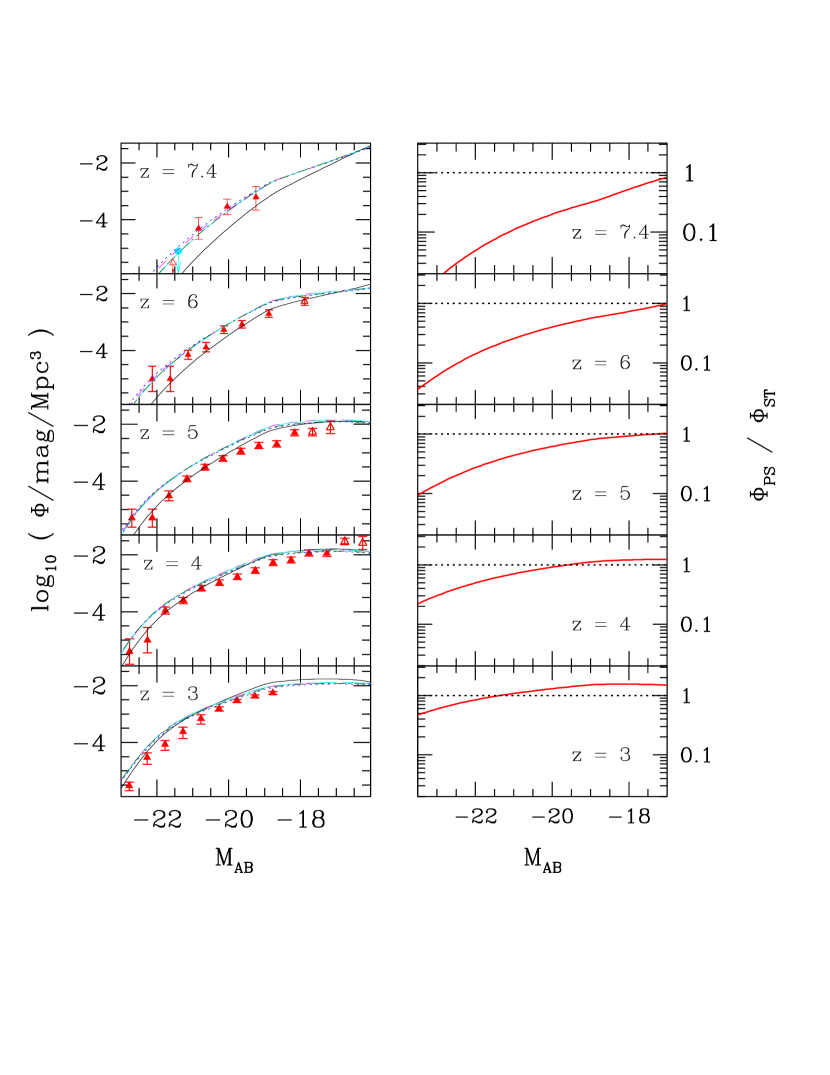
Figure 2: Left panels: The UV luminosity functions of LBGs at different redshifts. The observed data points are taken from Reddy & Steidel (2008) (triangles at $z=3$), Bouwens et al. (2007) (triangles at $z=4,~{}5$ & $6$) and Bouwens et al. (2008) (triangles at $z=7.4$). The upper limit at $z=7.4$ is taken from Mannucci et al. (2007) (the circle with an arrow). The solid (black) lines are for the PS mass function with Sasaki formalism. We have also shown the luminosity functions as predicted from ST (dotted blue), JW (short dashed magenta), Warren (long dash cyan) and Reed (dot short dash dark green) mass functions. Right panels: We show the ratio of the luminosity functions derived from the PS mass function to that from the ST mass function.

In this section we turn our attention to the UV luminosity function. First we illustrate the differences between results from different mass functions for fixed model parameters (see Fig. 2). Here, we do not make any attempt to fit the observed luminosity function. This will be done in the latter part of this section.

In our model we assume $f_{*}=0.3$, $\kappa=1.0$ with cosmological parameters mentioned in the introduction. We apply a constant dust reddening correction of factor $\eta=4.5$ for all redshifts and masses. It is clear from this figure that at $z\gtrsim 4$, the PS halo mass function (solid lines) predicts lower number of LBGs compared to any other mass functions in the observed luminosity range. This is simply a manifestation of the fact that the PS mass function predicts less number of rare high mass halos compared to other mass functions. But at the low mass end the PS mass function predicts a higher number density of collapsed objects. This effect can be seen at $z=3$ where the UV luminosity function at $M_{AB}\gtrsim-19$ is slightly higher for the models with PS mass function. The difference between the PS mass function and other mass functions are mass dependent which leads to a different slope in the luminosity function calculated from different mass functions. As expected all the other halo mass functions obtained from the simulation predict almost the same luminosity function at all redshifts. It is interesting to see that all the mass functions predict almost similar luminosity function at $z=3$ even though they are different at higher redshifts. As we pointed out before the slopes of the luminosity functions coming from different mass functions are indeed different.

In the right panels of Fig. 2 we show the ratio of luminosity function obtained from the PS mass function to that from the ST mass function. It is clear from the figure that there is a characteristics luminosity (or in turn the halo mass) for each redshift where the amplitude of the luminosity function derived from the PS and ST mass functions match with each other. However this characteristic luminosity increases with decreasing redshift. At $z\sim 3$, in the mass range of halos where star formation takes place the PS mass function over produces halos compared to the ST mass function (see Fig. 1). At the low mass range the excess is roughly a factor 2. The excess seen at the low end of the luminosity function produced by the PS mass function is due to this. At $M\sim 10^{12}~{}M_{\odot}$ all the models produce same number density at $z=3$. As star formation in halos above this mass are suppressed we do not see order of magnitude deviation in the high luminosity end as we would have expected from Fig. 1. However at $z\sim 5$, compared to the PS mass function the ST mass function produces a factor $\sim 2$ excess at $M=10^{12}~{}M_{\odot}$ and similar number of halos at the mass corresponding to $v_{c}=95~{}$km s^-1. Thus we see a much better matching at the low luminosity end of the luminosity function (see Fig. 2) and a very strong deviation at the high luminosity end for $z\gtrsim 5$.

Thus the reasonable match in the luminosity function at $z=3$ and strong disagreement at high-$z$ could be attributed to the fact that as one moves to higher and higher redshifts a given luminosity range is contributed by rarer and rarer objects (or higher $\sigma$ fluctuations; see Fig. 1) and the PS mass function is known to predict less number of rare objects compared to the ST mass function or other mass functions derived from simulations.

We find that the luminosity functions calculated using the derivative of the PS mass function and that obtained from the Sasaki formalism, differ negligibly for $\kappa=1$. However for $\kappa=0.1$ the Sasaki formalism predicts larger abundances by about $30\%$, in the observed luminosity range. The reason is as follows: first, the Sasaki formalism for $z=z_{c}$ gives the formation rate of halos, while the derivative gives the formation minus the destruction rate, and hence a lower net formation rate. Second, for any $\kappa$ we detect galaxies whose ages are $t_{a}\sim\kappa t_{\rm dyn}$, when they shine the maximum. In the Sasaki formalism, only a fraction of halos $p=D(t-t_{a})/D(t)$ formed at $(t-t_{a})$ survive at the observed time $t$. For small $\kappa$, we have $t_{a}/t\ll 1$, and thus $p\sim 1$ and the luminosity function predicted by the Sasaki formalism is higher, as its formation rate is higher. However as $\kappa$ increases, $t_{a}$ increases, $p$ decreases, and hence luminosity functions computed by the two methods first approach each other for $\kappa\sim 1$, after which the derivative method starts to produce a larger luminosity function. Nevertheless, since $t_{\rm dyn}$ is much smaller than the Hubble time, we find the differences between the luminosity function calculated by these two methods, are less than $30\%$ for all $z$. This difference is much smaller than the difference between luminosity functions, that are obtained using PS and other mass functions for $z>3$.

Figure 3: UV Luminosity functions of LBGs at different redshifts for the ST (solid lines) and PS (dashed lines) mass function. We fit the observed data points by changing $f_{*}/\eta$ using a $\chi^{2}$-fit. We ignore few data points in the low luminosity end (open triangles) while fitting as they suffer from completeness problem.

It is also clear from Fig. 2 that the shape of the UV luminosity functions (the slope and characteristic luminosity) and its redshift evolution, does depend on the assumed form of the halo mass function. This is expected as we have seen in Fig. 1 that the difference of halo formation rate coming out from different mass functions are mass dependent. Hence it suggests that, in principle we would be able to constrain the form of the halo mass function, just by fitting the luminosity functions. In what follows we use $\chi^{2}$ minimization to address this issue.

4.2 Best fit models: $\chi^{2}$ minimization

We use $\chi^{2}$ minimization technique to quantify how well the models using different mass functions reproduce the observed luminosity functions. For each redshift bin we have used the most recent measurement of the luminosity function that covers a wide range in luminosity. It is known that the estimations of luminosity function of LBGs suffer from the lack of redshift information and cosmic variance much more than typical Poisson errors (for example see Beckwith et al. 2006; Reddy et al. 2008; Bouwens et al. 2007; 2009). As $\chi^{2}$ minimization technique is sensitive to the errors, in our analysis we use errors that take care of the cosmic variance in addition to the Poisson error. We consider $f_{*}/\eta$ as the only free parameter. As this is assumed to be constant over the whole mass range, varying $f_{*}/\eta$ is like changing the mass to light ratio. Note that the observed luminosity functions are also given at different rest wavelength. For example at $z=$ 3, 4, 5, 6 and 7.4 the observed data points are obtained at $\lambda=$ 1700 Å, 1600 Å, 1600 Å, 1350 Å  and 1900 Å  respectively. In our models we take care of this aspect by calculating the intrinsic luminosity at appropriate wavelengths. The observed data and the best fit LF for the ST (solid line) and PS (dashed line) mass functions are given Fig. 3. The best fit parameters are summarized in Table 2.

For $z\sim 3$ we use the observed luminosity function given by Reddy & Steidel (2008) which covers the low luminosity end well. As this LF is obtained using several independent fields, the errors take into account the cosmic variance very well. As can be seen from the Table 2 the model using the ST mass function provides a good fit to the data (with a reduced $\chi^{2}_{\nu}=0.93$). Whereas the reduced $\chi^{2}$ for the model using the PS mass function is high ($\chi^{2}_{\nu}=3.90$). This is mainly because the PS mass function overpredicts low luminosity objects and under predicts high luminosity objects. This together with the incompleteness in the observational data used in Paper I prompted us to say in Paper I that one needs additional feedback to suppress the star formation in low mass halos that contribute to LF at the low luminosity end. However, it is clear now that for models with ST mass function, no additional feedback is needed to fit the luminosity function at $z\sim 3$. We also tried to fit the data by changing the characteristic mass scale for the AGN feedback. Even then the reduced $\chi^{2}$ for the best fitted models with the PS mass function are always larger than 2.

Table 2: The best fit values of $f_{*}/\eta$ for different redshifts. We show best fit parameters and $\chi^{2}$ per degree of freedom for models with both ST and PS halo mass functions.

	ST			PS
$z$	$f_{*}/\eta^{\dagger}$	$\chi^{2}_{\nu}$	$(f_{*}/\eta)_{1500}^{\ddagger}$	$f_{*}/\eta^{\dagger}$	$\chi^{2}_{\nu}$	$(f_{*}/\eta)_{1500}^{\ddagger}$
$3$	$0.066\pm 0.001$	$0.97$	$0.055$	$0.053\pm 0.001$	$3.90$	$0.044$
$4$	$0.049\pm 0.001$	$1.09$	$0.042$	$0.053\pm 0.001$	$2.32$	$0.046$
$5$	$0.040\pm 0.001$	$4.85$	$0.034$	$0.049\pm 0.001$	$8.28$	$0.042$
$6$	$0.036\pm 0.001$	$0.63$	$0.050$	$0.058\pm 0.002$	$1.19$	$0.081$
$7.4$	$0.111\pm 0.005$	$1.42$	$0.100$	$0.207\pm 0.009$	$2.27$	$0.186$
† $f_{*}/\eta$ obtained at the observed wavelength
‡ $f_{*}/\eta$ calculated at $\lambda=1500~{}$Å  considering a dust model similar to
that of our Galaxy or large Magellanic clouds (, 2003)

We now consider the luminosity functions for $z\sim 4$. The observed luminosity function at this redshift covers a much wider luminosity range, thanks to the Hubble Ultra deep field (HUDF) and GOODS (The Great Observatories Origins Deep Survey) data. Tabulated luminosity functions based on HUDF and GOODS are available in Beckwith et al. (2006) and Bouwens et al. (2007). We use Bouwens et al’s data for our analysis. They estimate rms due to cosmic variance to be $\sim 22$%. This fractional uncertainty is added to the Poisson error in quadrature (as done in Beckwith et al. 2006 and Bouwens et al 2009). We find that this is essential to get $\chi^{2}_{\nu}\sim 1$ while fitting even their best fitted Schechter function to the UV LF given in Table 5 of Bouwens et al. (2007). Also we ignore the last two data points at the low luminosity end (shown by the open triangles in Fig. 3) while fitting as these points are affected by incompleteness of the survey (Bouwens et al., 2007). Even for this redshift bin the model using the ST mass function provides better fit to the data than the one that uses the PS mass function. It is also interesting to note that $f_{*}/\eta$ is nearly constant for the model that uses the PS mass function between $z\sim 3$ and $z\sim 4$ but decreases for models using ST mass function.

The observed luminosity functions for $z\sim 5$ using HUDF are available in Oesch et al. (2007) and Bouwens et al. (2007). We use Bouwens et al’s data for our analysis. A fractional uncertainty of $\sim 18\%$ (Bowens et al. 2007) is added to the Poisson error in quadrature. We ignore the last two data points at the low luminosity end due to incompleteness (Bouwens et al., 2007). It is clear from Table 2 and Fig. 3 that the observed LF at this redshift is not reproduced well either by models using ST mass function or PS mass function. Observed points in the lower luminosity end are systematically lower than model predictions. In particular the discontinuity seen at $M_{AB}=-18.6$ contribute appreciably to the $\chi^{2}$. Note such a structure in LF, if true, can not be reproduced by our models. However, what is interesting is that for this redshift bin the model using the ST mass function provides better fit to the data than the one that uses the PS mass function.

The observed luminosity function at $z\sim 6$ are from Bouwens et al. (2007). A fractional uncertainty of $\sim 22\%$ (Bowens et al. 2007) is added to the Poisson error in quadrature. Models with both PS and ST mass functions provide acceptable fits to the data, with the latter having better reduced $\chi^{2}$. The observed luminosity function at $z\sim 7$ are from (Bouwens et al. 2009) and the published errors already account for the uncertainty due to small volume sampled. As the number of constraints are less models with both the mass function reproduce the data well.

The interesting result that emerges from the analysis presented till now is that the models with the ST mass function reproduce the observed LF much better than the ones that use the PS mass function. We also checked whether this result is valid if we use different observed luminosity functions. We find our best fit value of $f_{*}/\eta$ depends very much on the observed luminosity function we use (similar to what one finds for the Schechter function parameters). For example, for $4\leq z\leq 6$ the observed luminosity functions lack high precision measurements in the high luminosity end due to the small volume probed. Thus our best fit $f_{*}/\eta$ is decided by how well we fit the low luminosity end of the luminosity functions. However, ground based measurements which sample the high luminosity end well, tend to have slightly higher $f_{*}/\eta$. Ideally one should merge the ground and space based measurements by carefully accounting for all the possible biases. This is a non-trivial exercise and beyond the scope of this present work. However, irrespective of the data we used, we find invariably that the models with the ST mass function provide a better fit to the observed data. At least for $z\sim 3$, where the LF is well defined in the high luminosity end, we find that even changing the AGN feed back in model that uses PS mass function does not help in producing a $\chi^{2}$ better than that obtained for models with ST mass function.

We now consider the best fit values of $f_{*}/\eta$ at different redshifts. Columns 2 and 5 of Table 2 list the best fit values of $f_{*}/\eta$ obtained at the observed wavelength for which the luminosity function has been measured, for the models with the ST and PS mass functions respectively. Note that in principle, the amount of dust reddening correction depends very much on the wavelength. Hence, in order to compare the best fit values of $f_{*}/\eta$ at different redshifts we use the dust model like that applicable to the Galaxy or large Magellanic clouds (, 2003), and bring all the $f_{*}/\eta$ values to the wavelength of $1500$ Å. These values are also tabulated in Table 2 (in Column 4 and 7 for the models with the ST and PS mass functions respectively). It is clear from the table that no particular trend emerges at $3\leq z\leq 5$ though for higher redshifts an increase of $f_{*}/\eta$ may be needed. As already mentioned, the best fit values of $f_{*}/\eta$ very much depend on the observed luminosity function we have used. Also the nature of dust in the high redshift galaxies is very uncertain. Hence at this stage it is difficult to predict any trend on the values of $f_{*}/\eta$ and hence on the evolution of star formation in the high redshift galaxies. Future improved luminosity function measurements with reduced errors are needed to probe the redshift evolution of $f_{*}/\eta$. Nevertheless, as we noted above, it is heartening to find that a fairly simple model incorporating some of the physically motivated feedback effects and one free parameter $f_{*}/\eta$ does allow us to explain reasonably the observed UV luminosity function of high redshift LBGs.

Note that in Paper I we showed that the inclusion of star formation in the molecular cooled objects does not affect the UV luminosity function in the redshift range considered here. Hence we do not show any results of UV luminosity function for molecular cooled models. However, the molecular cooled objects play an important role in setting up the metallicity floor in the IGM at high redshift as shown in Paper II. Therefore, we will also consider the models with star formation in molecular cooled objects for galactic outflows.

5 Galactic outflows and the IGM

We turn now to models of galactic outflows and their feedback into the IGM, an issue that was addressed in detail in Paper II. Note that the metals detected in the IGM can only have been synthesized by stars in galaxies, and galactic outflows are the primary means by which they can be transported from galaxies into the IGM (Silk, Wyse & Shields, 1987, Tegmark, Silk & Evrad 1993, Miralda-Escude & Rees, 1997, Nath & Trentham, 1997, Madau, Ferrara, Rees 2001, Furlanetto & Loeb 2003, Scannapieco 2005, Bertone, Stoehr & White 2005, Oppenheimer & Dave 2006, Bertone, De Lucia & Thomas 2007). The mechanical energy that drives outflows arises from the supernovae (SNe) explosions associated with the star formation activities in the galaxy. We concentrate on how much of the IGM can be polluted by the outflows from galaxies and also what would be the metallicity of those polluted regions. We follow Paper II in modelling galactic outflows and their feedback effects. Here we briefly outline this procedure.

First, the star formation rate of an individual galaxy is converted to the rate of SNe. This depends on the assumed IMF. For the IMF used in this work, one SNe is produced per 50 solar mass of star formation. A single SNe is assumed to produce $10^{51}$ erg of energy out of which a fraction $\epsilon_{w}=0.1$ goes into the outflow. The outflow is taken to be spherically symmetric and its dynamics is followed using a thin-shell approximation (see Eqs. (5)-(16) of Paper II for the details). The dark matter potential of the halo is assumed to be in NFW profile and a fraction ($f_{h}=0.10$) of the total baryonic mass is taken to be in thermal equilibrium at virial temperature in this potential. The amount of mass coming out of the star forming region is assumed to be proportional to the mass of stars formed with the proportionality constant $\eta_{w}=0.3$. We also assume that $90\%$ of the shocked IGM/halo gas is concentrated in the thin-shell region and rest $10\%$ is incorporated in the hot bubble. The initial radius of the shell is taken to be $1/10$ the virial radius, and the outflow is frozen to the Hubble flow when its peculiar velocity drops to the sound speed of the surrounding IGM.

The extent $R_{s}$, to which an individual outflow can propagate into the IGM, depends mainly on the rate of SNe productions and the energy efficiency of the outflow, $\epsilon_{w}$. In Paper II, we showed that $R_{s}$ is fairly independent of other parameters as long as the outflow escapes the halo potential. Note that we have already constrained $f_{*}/\eta$ by fitting the UV luminosity functions of LBGs. However, we need some specific values of $f_{*}$ to calculate the effect of outflow. For the PS mass function we take $f_{*}=0.30$ and for ST and other mass functions $f_{*}=0.25$ for the whole $z$ range.

After calculating the evolution of a suite of individual outflow models, we can study several global properties of the wind affected regions. One simple quantity is the porosity $Q(z)$, which is a measure of the (volume) fraction of the universe affected by outflows. This is calculated by adding up the outflow volumes around all the sources at any redshift:

$$Q(z)=\int\limits_{M_{\rm low}}^{\infty}{\rm d}M\int\limits_{z}^{\infty}{\rm d}z_{c}~{}{\cal N}(M,z_{c})~{}\frac{4}{3}\pi\left[R_{S}(1+z)\right]^{3}.$$ (13)

Here, $R_{s}(M,z,z_{c})$ is the radius of an outflow at redshift $z$, arising from a halo of mass $M$ which collapsed at redshift $z_{c}$. This comes from solving for the outflow dynamics. Note that in the Sasaki formalism as applied to the PS mass function, one has to replace ${\cal N}(M,z_{c})$ by ${\cal N}_{s}(M,z,z_{c})$ (see Paper II). For $Q<1$ the porosity gives the probability that a randomly selected point in the universe at $z$ lies within an outflow region. For $Q\sim 1$, it is more useful to define the associated filling factor of the outflow regions, which if outflows are randomly distributed is given by, $F=1-\exp[-Q(z)]$. One can also calculate porosity weighted averages of various physical quantities associated with the outflows, and their probability distribution functions (PDFs). In our models, we compute the metallicity of the outflowing gas and the global average metallicity assuming instantaneous metal mixing within the galaxy (see appendix A of Paper II).

Figure 4: The volume filling factor of the IGM by the outflows for models with different halo mass functions. The dotted (red), long dashed (green), short dashed (blue), dot dot dashed (magenta) and dotted dashed(violet) curves are for the model with the derivative of the PS, ST, JW, Warren and Reed mass function respectively. We also show the filling factor calculated using the Sasaki formalism of the PS mass function with thick solid (black) line. The thin solid (black) line is obtained assuming no destruction of outflows, and the formation rate of halos from the Sasaki formalism applied to the PS mass function.

In Fig. 4 we show the filling factor of the universe as predicted by using different halo mass functions. The different models considered are: the ST (long dashed green), JW (short dashed blue), Warren (dot dot dashed magenta) and Reed (dotted dashed violet) halo mass functions. In all these models we assume $f_{*}=0.25$. For comparison we also show the filling factor as calculated from the the PS mass function using both the Sasaki formalism (thick solid black line) and by taking the derivative to compute the net formation rate (the short dashed red line). Recall that in these models we take $f_{*}=0.30$. It is clear that all the models which employ the derivative ${\cal N}$ to characterise the net halo formation rate, predict similar results for the volume filling factor (with in 10%), with $F$ of order $0.7-0.8$ at $z=3$. However the model using the Sasaki formalism and the PS mass function predicts a lower volume filling factor ($F=0.55$ at $z=3$). At $z\gtrsim 6$ the difference in $F$ is like 30% where as at $z\lesssim 3$ the difference is about 50%. We find as in Paper II that outflows from halos in the mass range $M\sim 10^{7}-10^{9}~{}M_{\odot}$ dominate the volume filling factor.

It is interesting that for the PS mass function, the volume filling factor is different for the two ways of calculating the net formation rate, namely the derivative and the Sasaki formalism.

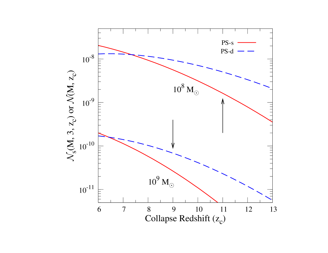
Figure 5: Comparison of formation rate of the dark matter halos as obtained from Sasaki formalism of the PS mass function (solid line) and that calculated by taking the derivative (dashed line) for $10^{8}~{}M_{\odot}$ and $10^{9}~{}M_{\odot}$ halos. The rates are in arbitrary units. We fixed the observed redshift $z=3$. The arrows indicate the typical collapsed redshifts for these halos.

This obtains although there was hardly any difference in the UV luminosity function calculated from these two methods. The reason behind this can be understood as follows. In case of Sasaki formalism whenever a halo is destroyed, one implicitly assumes that the outflowing material no longer contributes to the volume filling factor. But in the models with the derivative of the PS mass function once an outflow is formed it contributes to the volume filling factor for ever ; although the derivative itself gives the net (formation minus destruction) rate, at $z_{c}$. And thus leads to a smaller formation rate of halos at $z_{c}$. The net difference between Sasaki formalism and the derivative of the PS mass function can be seen from Fig. 5.

In this figure we show ${\cal N}_{s}(M,z,z_{c})$ and ${\cal N}(M,z_{c})$ as a function of $z_{c}$ for $10^{8}~{}M_{\odot}$ and $10^{9}~{}M_{\odot}$ halos, while fixing $z=3.0$. Note that ${\cal N}_{s}(M,z,z_{c})$ and ${\cal N}(M,z_{c})$ come as a part of the integrand over $z_{c}$ while calculating the porosity of the galactic outflows at a given $z$ (Eq. 13). We choose these values of $M$ as outflowing material from halos with such masses dominate the volume filling factor of IGM, as mentioned above. It is clear from the figure that at typical collapsed redshifts for such halos (as indicated with the arrows) the derivative of the PS mass functions predicts about a factor of $3$ higher net formation rate compared to that of Sasaki formalism applied to the PS mass function. This difference decreases with decreasing $z_{c}$ and at certain redshift the Sasaki formalism predicts higher formation rate (weighted by the destruction probability) compared to the derivative. However the star formation in halos with these masses would be suppressed by the radiation feedback due to reionization at $z_{c}<$6. Therefore, at $z=3$, the integrand in Eq. 13 will be larger for the PS derivative compared to that obtained from Sasaki formalism (for the range of halo masses and $z_{c}$ that contributes dominantly to $F$). For this reason the model with the derivative of the PS mass function predicts higher volume filling factor even if the UV luminosity function predicted by them were same.

Note that when we use the Sasaki formalism, we could go to the other extreme and not destroy any outflow, by replacing the survival probability, $D(z)/D(z_{c})$, with unity. In this case we find that the volume filling factor is the largest, even higher than that obtained when one uses the derivative of the mass function to calculate the halo formation rate. We show this as a thin solid line in Fig. 4. The volume filling factor that realistically obtains will be bracketed by these two cases (the thick/thin solid lines of Fig. 4). This difference also gives an estimate of the uncertainty in the volume filling factor obtained in semi-analytic models.

We see from Fig 1 that the net formation rates, calculated using the derivative of all the mass functions, agree reasonably well, for halos that contributes dominantly to $F$. This is the reason behind the close agreement behind $F$ estimated using the derivative of different mass functions.

Next we compare various physical properties of outflows for different halo mass functions.

Figure 6: The global properties of outflows for the derivative (dashes) and Sasaki formalism (dotted dashes) of the PS mass function. We also show for the derivative of the ST mass function with solid lines. Panel (a) shows the volume filling factor $F$. In panel (b) and (c) we show the porosity weighted average dark matter mass (in $M_{\odot}$) and comoving radius (in kpc) respectively. In panel (d) we show the global average metallicity produced by star formation (the top set of curves), and that injected into the IGM (the lower set of curves). The porosity weighted average peculiar velocity (in km s^-1) and hot bubble temperature of the outflows are shown in panel (e) and (f) respectively.

In Fig. 6 we show various physical parameters related to outflows for the derivative of the PS (dashed) and ST (solid) mass function. For comparison we also show the results for the Sasaki formalism of the PS mass function with dotted dashed line. In panel (a) we compare the filling factor that we have already discussed in great details. Panel (b) compares the porosity weighted average mass of the dark matter halos that contribute to the filling factor. Since the ST mass function predicts more high mass objects, the average halo mass that contribute to the filling factor predicted by this model is slightly higher compared to the PS mass function for $z\gtrsim 3$. However, vary massive halos which formed at lower redshifts do not have an outflow due to smaller value of $f_{*}$. Hence at $z\lesssim 3$ average mass contributed to the volume filling factor is less in the models with the ST mass function compared to that with the PS mass function. Panel (c) compares the porosity weighted average radius of outflows whereas panel (d) compares the global average metallicity produced by star formation (the top set of curves), and that which is injected into the IGM (the lower set of curves). Due to the reason already mentioned above, the average radius of the outflow and the metallicity show a similar behavior as the average halo mass for different models. In panel (e) and panel (f) we show the porosity averaged peculiar velocity of the outflow and the temperature of the hot bubble respectively. Both the average peculiar velocity and the temperature are higher in case of the Sasaki formalism mainly reflecting the fact that $f_{*}$ is higher for the PS mass function compared to the ST mass function. For the PS mass function, although the Sasaki formalism and the derivative have the same $f_{*}$ the average peculiar velocity and the temperature are lower in the model with the derivative due to the higher volume filling factor. In general, we conclude from Fig. 6 that even if the filling factor changes depending on the way we calculate the net formation rate (upto 50% change), the physical properties related to the outflow do not vary significantly between these models. As mentioned earlier, an important invariant feature of all the outflow models is that small mass halos with $M\sim 10^{7}-10^{9}M_{\odot}$ contribute dominantly to the porosity $Q(z)$ (as originally discussed by Silk, Wyse & Shields, 1987, Miralda-Escude & Rees, 1997, Nath & Trentham, 1997, Madau, Ferrara & Rees, 2001).

The mildly overdense regions which produce the Lyman-$\alpha$ forest lines probe the power spectrum of density perturbations down to a comoving scale of half a Mpc or so at $z\sim 3$. In Paper II we found that in the atomic cooled models, the IGM is polluted by regions of hot gas ($T\sim 10^{5}$ K) with sizes of $200-800$ kpc. This could potentially distort the density power spectrum as inferred from the Lyman-$\alpha$ forest. There is no evidence in the current data for such distortions. However, this aspect needs to be studied further to see how much of a problem this is for the above models.

On the other hand, we also noted that molecular cooled models are better placed to seed the IGM with metals without strong distorting effects on the Lyman-$\alpha$ forest lines. This is because outflows from molecular cooled halos can significantly fill the universe, even at $z\sim 8$, while at the same time having typically a much smaller radius. We therefore also consider here the effect of changing the halo mass function in such models.

Figure 7: Volume filling factor as obtained from molecular cooled models. The solid and dashed lines are for the models with derivative of the ST and PS mass function. The dotted-dashed line show the volume filling factor as obtained from Sasaki formalism of the PS mass function.

In Fig. 7 we show the volume filling factor predicted by the molecular cooled models, as obtained from the models with derivative of the PS (dashed) and ST (solid) mass function. We also show the $F(z)$ when we use the Sasaki formalism and the PS mass function (dotted dashed line). We take $f_{*}=0.05$ in the molecular cooled halos in order to be consistent with the optical depth of reionization inferred from the CMB polarization measurements (see Table 1). As expected all these models fill the IGM with outflows and metals at fairly high redshift ($z\gtrsim 8$). The volume filling factor is again smaller when one employs the Sasaki formalism, essentially for the same reason as discussed in the case of atomic cooled models. The higher value of $f_{*}$ in the model with the derivative of the PS mass function compared to the model with the derivative of the ST mass function makes the volume filling factor larger for the former model. We have also checked that physical parameters in these models are similar to that obtained in the molecular cooled models discussed in Paper II. Hence the conclusions about the molecular cooled models arrived at in Paper II remain; that they are more favorable in spreading the metals, without unduly distorting the Lyman-$\alpha$ forest.

6 Discussions and Conclusions

In a series of papers (Paper I and Paper II) we have been developing semi-analytic models of star formation and associated outflows in high redshift galaxies that are constrained by available observations on UV luminosity function and reionization. Our models successfully explained the observed UV luminosity functions of Lyman break galaxies at $z\geq 3$ and predicted various effects of outflows form the galaxies on the metal enrichment of the IGM. In all these models one of the main ingredients is the halo mass function. We used the standard PS mass function with the halo formation rate given by Sasaki (1994). However the halo mass functions determined by fitting various numerical simulations of galaxy formation differ considerably from the PS mass function, especially for rare objects. It is then necessary to examine how this affects the model predictions given in Paper I and II. Here, we present a systematic comparison of the results for different analytical forms of the halo mass functions.

Further, two methods are normally used in the literature to compute the net formation rate of halos for the PS mass function; (i) the formalism of Sasaki is used to calculate a formation rate of halos at collapse and then fold in the halo survival probability to later epochs, or (ii) the derivative of the PS mass function is employed to get a net formation rate (formation rate minus destruction rate) at any redshift. We had employed the Sasaki formalism for the PS mass function in Paper I and II. Here we also calculate model predictions using the derivative of the PS mass function to test the sensitivity of the results to the manner of computing the net halo formation rate. Such a comparison is also important as the Sasaki formalism is not easily generalizable to other mass functions. For all other halo mass functions one has to simply take recourse to its derivative, to model the net formation rate of halos.

We first show, by comparing the derivatives of all mass functions, that the historically used Press-Schechter mass function predicts a lower formation rate of rare high mass dark matter halos compared to any other mass function. However, all other mass functions do not differ significantly in the formation rate of collapsed dark matter halos. Therefore, significant differences can arise in model predictions made using the PS mass function and the other forms of the mass functions considered here. We show the effect of this difference by (i) calculating the reionization history of the universe, (ii) fitting the observed UV luminosity functions of high redshift LBGs, and (iii) calculating the feedback of star formation on the IGM. The main results of our study are as follows:

• In order to produce a given electron optical depth to the reionization, the efficiency in the star formation and/or in UV escape fraction has to be lower in the models using ST and other mass functions obtained from simulations compared to that with the PS mass function. This decrease has to be much more in the small mass molecular cooled halos if they also contribute to the reionization process.

• All new sets of data points, which extend the UV luminosity function of LBGs to the faint end and to higher $z$, can be naturally explained in the framework of our earlier models.

• The luminosity function determined using the PS and ST mass functions match reasonably at $z=3$, but they differ more and more strongly as one goes to higher redshifts, and especially at the bright end (right panel of Figure 2). This is because as one moves to higher and higher redshifts a given luminosity range is contributed by rarer and rarer objects and the PS mass function predicts a lower net formation rate compared to the ST mass function or other mass functions derived from simulations. The UV luminosity functions determined from all mass functions, other than the PS mass function, agree reasonably with each other.

• We find that the luminosity functions calculated using the derivative of the PS mass function and that obtained from the Sasaki formalism, differ negligibly for $\kappa=1$ and by less than $30\%$ for other values of $0.1<\kappa<4$.

• We show, by using $\chi^{2}$ minimization technique, that the models with the ST halo mass function provide a better fit to the observed UV luminosity functions in the redshift range $3\leq z\leq 7.4$ compared to the models with the PS halo mass function. However, the redshift evolution of the best fit model parameter $f_{*}/\eta$ crucially depends on the data set used, as well as various uncertainties such as k-correction, dependence of dust opacity on the wavelength etc.

• Models with different mass functions, using the derivative of the mass functions to calculate the net formation rate of halos, predict very similar (with in 10%) volume filling factor for metals in the IGM. However, these models always predict a higher volume filling factor compared to the Sasaki formalism of the PS mass function. Therefore, even though the method used to calculate the formation rate of collapsed dark matter halos has only a mild effect on the predictions of high redshift UV luminosity functions, they do predict different outflow feedback to the IGM. Different models give similar predictions for other physical parameters associated with outflows and the conclusions of Paper II appear to be largely insensitive to the adopted form of the halo mass function.

The next important step in the development of our models could be to implement it in the framework of a numerical simulation or by generating merger trees. This will help in unambiguously determining the halo formation rate and its survival probability. However, as mentioned earlier, one has to resolve the formation of halos right from $10^{7}M_{\odot}$ to $10^{12}M_{\odot}$ in order to model both IGM metal enrichment and the galactic luminosity function. To achieve such a large dynamic range would be a major challenge.

References

- (1) Barkana, R., Loeb, A. 2001, PhR, 349, 125
- (2) Beckwith, S. V. W., et al., 2006, AJ, 132, 1729
- (3) Benson, A. J., Lacey, C. G., Baugh, C M., Cole, S., Frenk, C. S., 2002, MNRAS, 333, 156
- (4) Bertone, S., De Lucia, G., Thomas, P. A., 2007, MNRAS, 379, 1143
- (5) Bertone, S., Stoehr, F., White, S. D. M, 2005, MNRAS, 359, 1201
- (6) Best, P. N., Kaiser, C. R., Heckman, T. M., Kauffmann, G., 2006, MNRAS, 368, L67
- (7) Bouwens R., Illingworth G., 2006, NewAR, 50, 152
- (8) Bouwens, R. J., Illingworth, G. D., Franx, M., Ford, H., 2007, ApJ, 670, 928
- (9) Bouwens, R. J., Illingworth, G. D., Franx, M., Ford, H., 2008, arXiv:0803.0548
- (10) Bower, R. G., Benson, A. J., Malbon, R., Helly, J. C., Frenk, C. S., Baugh, C. M., Cole, S., Lacey, C. G., 2006, MNRAS, 370, 645
- (11) Bromm, V., Loeb A., 2002, ApJ, 575, 111
- (12) Cole, S., Aragon-Salamanca, A., Frenk, C. S., Navarro, J. F., Zepf, S. E., 1994, MNRAS, 271, 781
- (13) Chiu W. A., Ostriker J. P., 2000, ApJ, 534, 507
- (14) Dijkstra, M., Haiman, Z., Rees, M., Weinberg, D. H., 2004, ApJ, 601, 666
- (15) Dunkley, J. et al., 2008, arXiv:0803.0586
- (16) Fan, X., Strauss, M. A., Richards, G. T. et al., 2006, AJ, 131, 1203
- (17) Furlanetto, S., R., Loeb, A., 2003, ApJ, 588, 18
- (18) Gabasch, A., et al., 2004, A&A, 421, 41
- (19) Gordon, K. D., Clayton, G. C., Misselt, K. A., Landolt, A. U., Wolff, M. J., 2003, ApJ, 594, 279
- (20) Giavalisco, M., 2005, New Astronomy Review, 49, 440
- (21) Haehnelt, M. G., Rees, M. J., 1993, MNRAS, 263, 168.
- (22) Iwata I., Ohta K., Tamura N., Akiyama M., Aoki K., Ando M., Kiuchi G., Sawicki M., 2007, MNRAS, 376, 1557
- (23) Jenkins, A., Frenk, C. S., White, S. D. M., Colberg, J. M., Cole, S., Evrard, A. E., Couchman, H. M. P., Yoshida, N., 2001 MNRAS, 321, 372
- (24) Kauffmann, G., White, S. D. M., Guiderdoni, B., 1993, MNRAS, 264, 201
- (25) Madau, P., Ferrara, A., Rees, M., 2001, ApJ, 555, 92
- (26) Mannucci, F., Buttery, H., Maiolino, R., Marconi, A. & Pozzetti, L. 2007, A&A, 461, 423
- Miralda-Escude & Rees (1997) Miralda-Escude, J., Rees, M. J., 1997, ApJ, 478, 57
- (28) Nagamine K., Ostriker, J. P., Fukugita, M., Cen, R., 2006, astro-ph/0603257
- (29) Nath, B. B., & Trentham, N., MNRAS, 291, 505
- (30) Oesch, P. A., et al., 2007, ApJ, 671, 1212
- (31) Oppenheimer, B. D., Dave, R., 2006, MNRAS, 373, 1265
- (32) Ouchi, M., et al., 2004, ApJ, 611, 660
- (33) Padmanabhan T, Theoretical Astrophysics, 2002, Volume I, Cambridge University Press
- (34) Paltani, S., et al., 2007, A&A, 463, 873
- (35) Peebles P., 1993, Principles of Physical Cosmology. Princeton Univ. Press, Princeton, NJ, USA
- (36) Press W. H., Schechter P., 1974, ApJ, 187, 425
- (37) Reed, D. S., Bower, R., Frenk, C. S., Jenkins, A., Theuns, T., 2007, MNRAS, 374, 2
- (38) Reed D., Gardner J., Quinn T., Stadel J., Fardal M., Lake G., Governato F., 2003, MNRAS, 346, 565
- (39) Reddy, N. A., Steidel, C. C., Fadda, D., Yan, L., Pettini, M., Shapley, A. E., Erb, D. K., Adelberger, K. L., 2006, ApJ, 644, 792
- (40) Reddy, N. A., Steidel, C. C., 2008, arXiv:0810.2788
- (41) Ripamonti, E., 2007, MNRAS, 376, 709.
- (42) Samui, S., Srianand, R., Subramanian, K., 2007, MNRAS, 377, 285
- (43) Samui, S., Subramanian, K., Srianand, R., 2008, MNRAS, 385, 783
- (44) Sasaki S., 1994, PASJ, 46, 427
- (45) Sawicki, M., & Thompson, D., 2006, ApJ, 642, 653
- (46) Scannapieco, E., 2005, ApJ, 624, L1
- (47) Sheth R. K., Tormen G., 1999, MNRAS, 308, 119 (ST)
- (48) Silk, J., Wyse, R. F. G., Shields, G. A., 1987, ApJ, 322, 59
- (49) Somerville, R. S., Primack, J. R., 1999, MNRAS, 310, 1087
- (50) Somerville, R. S., Primack, J. R., Faber, S. M., 2001, MNRAS, 320, 504
- (51) Steidel, C. C., Adelberger, K. L., Giavalisco, M., Dickinson, M. and Pettini, M., 1999, ApJ, 519, 1
- (52) Tegmark, M., Silk, J., Evrard, A., 1993, ApJ, 417, 54
- (53) Thoul A. A., Weinberg D. H., 1996, ApJ, 465, 608
- (54) Warren M., Abazajian K., Holz D., Teodoro L., 2006, ApJ, 646, 881
- (55) White S. D. M., Frenk C. S., 1991, ApJ, 379, 52
- Yoshida, M. (2004) Yoshida, M., et al., 2006, ApJ, 653, 988