Interstellar Extinction Law toward the Galactic Center III :
$J$, $H$, $K_{S}$ bands in the 2MASS and the MKO systems,
and 3.6, 4.5, 5.8, 8.0 $\mu$m in the Spitzer/IRAC system

Abstract

We have determined interstellar extinction law toward the Galactic center (GC) at the wavelength from 1.2 to 8.0 $\mu$m, using point sources detected in the IRSF/SIRIUS near-infrared survey and those in the 2MASS and Spitzer/IRAC/GLIMPSE II catalogs. The central region $\mid l\mid\lesssim 3\fdg 0$ and $\mid b\mid\lesssim 1\fdg 0$ has been surveyed in the $J$, $H$ and $K_{S}$ bands with the IRSF telescope and the SIRIUS camera whose filters are similar to the Mauna Kea Observatories (MKO) near-infrared photometric system. Combined with the GLIMPSE II point source catalog, we made $K_{S}$ versus $K_{S}-\lambda$ color-magnitude diagrams where $\lambda=$ 3.6, 4.5, 5.8, and 8.0 $\mu$m. The $K_{S}$ magnitudes of bulge red clump stars and the $K_{S}-\lambda$ colors of red giant branches are used as a tracer of the reddening vector in the color-magnitude diagrams. From these magnitudes and colors, we have obtained the ratios of total to selective extinction $A_{K_{S}}/E_{K_{S}-\lambda}$ for the four IRAC bands. Combined with $A_{\lambda}/A_{K_{S}}$ for the $J$ and $H$ bands derived by Nishiyama et al., we obtain $A_{J}:A_{H}:A_{K_{S}}:A_{[3.6]}:A_{[4.5]}:A_{[5.8]}:A_{[8.0]}=3.02:1.73:1:0.50:0.39:0.36:0.43$ for the line of sight toward the GC. This confirms the flattening of the extinction curve at $\lambda\gtrsim 3\mu$m from a simple extrapolation of the power-law extinction at shorter wavelengths, in accordance with recent studies. The extinction law in the 2MASS $JHK_{S}$ bands has also been calculated, and a good agreement with that in the MKO system is found. Thus, it is established that the extinction in the wavelength range of $J$, $H$, and $K_{S}$ is well fitted by a power law of steep decrease $A_{\lambda}\propto\lambda^{-2.0}$ toward the GC. In nearby molecular clouds and diffuse interstellar medium, the lack of reliable measurements of the total to selective extinction ratios hampers unambiguous determination of the extinction law; however, observational results toward these lines of sight cannot be reconciled with a single extinction law.

1 Introduction

The absolute value of interstellar extinction to an individual star is difficult to determine, and so is its wavelength dependence. Toward the Galactic center (GC), however, we can directly derive the wavelength dependence of interstellar extinction, assuming only that the center of stellar distribution in the lines of sight is at the same distance from us and that the foreground extinction is patchy; such a principle has been employed for star clusters and is referred to as the cluster method or variable-extinction method (Krełowski & Papaj, 1993). By plotting the apparent magnitude versus the color excess of a group of stars, one obtains a straight line with the slope equal to the total to selective extinction ratio, e.g., $A_{K_{S}}/E_{H-K_{S}}$. This variable-extinction method was applied for the red clump (RC) stars around the GC by Woźniak & Stanek (1996) at $V$ and $I$, and by Nishiyama et al. (2006, 2008) as the “RC method” at $V$, $J$, $H$, and $K_{S}$.

Nishiyama et al. (2006) measured the peak position of the RC stars in the color-magnitude diagram (CMD) of each small ($\sim 4\arcmin\times 4\arcmin$) field in their survey area of $\mid l\mid\leq 2\arcdeg$ and $\mid b\mid\leq 1\arcdeg$, and the reddening and the extinction were derived from the relative shifts of the peak color and the peak magnitude, respectively. Here the most important point is that the magnitude of extinction accompanied by a certain amount of reddening can be derived exactly, as long as no difference in 1) the mean distance, 2) the mean absolute magnitude, and 3) the mean color of the RC population exists among the small fields. Since the survey is deep enough and the survey area of a few degrees (projected area of a few hundred pc at the GC) does not seem to have different RC population correlated with the amount of foreground extinction, this assumption is reasonable. The ratios of total to selective extinction, $A_{K_{S}}/E_{H-K_{S}}$, $A_{K_{S}}/E_{J-K_{S}}$, and $A_{H}/E_{J-H}$ were in turn used to derive the wavelength dependence of extinction $A_{J}:A_{H}:A_{K_{S}}$. When approximated as a power law of the wavelength $\lambda$, the interstellar extinction $A_{\lambda}$ toward the GC decreases as $\lambda^{-1.99}$ in the wavelength range of $J$, $H$, and $K_{S}$, being steeper to the longer wavelength than the Rieke & Lebofsky (1985) result $\lambda^{-1.6}$.

Direct measurements of extinction are extremely difficult because of the uncertainty of the distance of light sources. Therefore, the ratios of reddening (ratios of color excesses; e.g., $E_{\lambda-V}/E_{B-V}$) are generally determined first, and then these color excess ratios are transformed into the absolute extinction $A_{\lambda}$ with some assumptions. For this purpose, the total to selective extinction ratio $A_{V}/E_{B-V}=R_{V}$ is often derived somehow, either by extrapolation of the color excess diagram to the longer wavelength or by a certain assumption, and then employed with the equation

$$\frac{A_{\lambda}}{E_{B-V}}=\frac{E_{\lambda-V}}{E_{B-V}}+R_{V}.$$ (1)

So long as one compares the color excesses, which are obtained directly and accurately, meaningful comparison is possible for different determinations, and many attempts have been made in this color-color method. However, caution must be exercised in the use of absolute extinction $A_{\lambda}$.

Rieke & Lebofsky (1985) determined the extinction law toward the GC from 1 to 13 $\mu$m by the color excess observations of five supergiants near the GC and $o$ Sco. They first set $E_{V-K}/E_{B-V}=2.744$ for all the stars and assumed $A_{V}/E_{B-V}=3.09\pm 0.3$ for the extinction toward the GC. The lower limit of total to selective extinction ratio 3.09 was determined from the decrease of extinction in the range of $L,M,8~{}\mu$m, but the observation at these wavelengths was relatively uncertain. Longward of 3 $\mu$m, Lutz et al. (1996) and Lutz (1999) observed hydrogen recombination line emission toward the GC with the Infrared Space Observatory SWS instrument and found that the extinction curve is much flatter than the Rieke & Lebofsky (1985) results. Lutz et al. (1996) compared the observed fluxes and expected fluxes predicted for the HII region in an aperture of $14\arcsec\times 20\arcsec$ centered on Sgr A^∗. They confirmed the applicability of the case B conditions from the observations of different upper-level lines. It should be noted, however, that Lutz et al. (1996) had to assume a $K$ band extinction of 3.47 mag because the ratio of reddening, not the absolute extinction, in the hydrogen line strengths were derived also in their determination.

The wavelength dependence of interstellar extinction toward the GC, therefore, can be summarized as follows. The extinction in the near-infrared wavebands $J,H,K_{S}$ is fitted well by a steep power law $\lambda^{-2}$, but decreases only slightly beyond $\lambda=3~{}\mu$m, and then shows a large maximum due to the silicate absorption at $\lambda=9.7~{}\mu$m. The steep power law in the wavelength range $1-2.5~{}\mu$m and flat curve in $3-4~{}\mu$m is consistent with the polarimetry results (Nagata et al., 1994), which can be regarded, in a sense, as an absolute determination of the difference between the extinctions of two orthogonal axes.

In directions of other than the GC, flat extinction dependence in the wavelength range of $3-8~{}\mu$m has also been derived. Indebetouw et al. (2005) measured the mean color excess ratios from the color distributions of stars observed with the Infrared Array Camera (IRAC; Fazio et al., 2004) on board Spitzer Space Telescope (SST), along two lines of sight in the Galactic plane. Investigations toward five nearby star-forming regions (Flaherty et al., 2007) and the star-forming dense core Barnard 59 (Román-Zúñiga et al., 2007) also suggest relatively flat extinction curves from 3 to 8 $\mu$m. All these studies obtained color ratios, either $E_{\lambda-K_{S}}/E_{J-K_{S}}$ or $E_{\lambda-K_{S}}/E_{H-K_{S}}$, first. Then these color excess ratios are transformed into the absolute extinction ratio (e.g., $A_{\lambda}/A_{K_{S}}$) on the assumption of one ratio (e.g., $A_{H}/A_{K_{S}}$) using the equation

$$\frac{A_{\lambda}}{A_{K_{S}}}=\left(\frac{A_{H}}{A_{K_{S}}}-1\right)\frac{E_{\lambda-K_{S}}}{E_{H-K_{S}}}+1.$$ (2)

Assuming their distribution in the Galactic plane, Indebetouw et al. (2005) fitted the locus of RC stars in a color magnitude diagram and derived $A_{H}/A_{K_{S}}=1.55\pm 0.1$. Then using the equation (2), Indebetouw et al. (2005), Román-Zúñiga et al. (2007), and Flaherty et al. (2007) derived the absolute extinction ratios. As pointed out by Indebetouw et al. (2005), such extinction ratios of $A_{H}/A_{K_{S}}$ on the assumption of the RC star location in the Galactic plane might be more accurate than the extrapolation of the $E_{\lambda-K_{S}}/E_{J-K_{S}}$ curve toward the longer wavelength to get the absolute extinction values as in equation (1), but one should keep in mind that the assumption of the one ratio can lead to large errors in $A_{\lambda}/A_{K_{S}}$. Color excess ratios with the SST/IRAC bands are different between the star forming regions and the diffuse interstellar medium, and a difference in the extinction law between them was suggested (Flaherty et al., 2007).

In this paper, we assume that the center of distribution in the lines of sight is at the same distance from us for the RC giants and the giants in the upper red giant branch (RGB), and determined the total to selective extinction ratios $A_{K_{S}}/E_{K_{S}-\lambda}$ for the IRAC wavebands while we use the IRSF/SIRIUS (similar to the the Mauna Kea Observatories (MKO) near-infrared photometric system; Tokunaga et al., 2002) survey results for the $K_{S}$ band. Also, using the RC and upper RGB stars toward the GC, the total to selective extinction ratios $A_{K_{S}}/E_{J_{2MASS}-K_{S}}$, $A_{K_{S}}/E_{H_{2MASS}-K_{S}}$, and $A_{K_{S}}/E_{K_{2MASS}-K_{S}}$ in the Two Micron All Sky Survey (2MASS) bands were derived, and the agreement to the steep extinction law determined by Nishiyama et al. (2006) is examined in the 2MASS bands. We compare these results with the previous determination of interstellar reddening in different lines of sight, and discuss their difference.

This variation of the “RC method” is unique and different from any previous determinations of mid-infrared extinction because it is free from the transformation equations (1) and (2). It is on the assumptions of the same mean distance and magnitude of the RC star population among the small fields, of the agreement of the central positions of the spatial distributions of the RC and RGB stars, and that the upper RGB stars have colors varying only with luminosity. The distance to the RC stars seem to be rather constant (Nishiyama et al., 2005) in this range of Galactic longitudes, and it seems reasonable to assume that the RC and RGB stars have similar spatial distributions. The upper RGB has been used for determining the interstellar reddening and extinction by many investigators. Frogel et al. (1999) used RGB stars with the unreddened $K$ magnitude range of 8.0 to 12.5. They compared the RGB colors of the inner bulge ($|l|<4\arcdeg,|b|<3\arcdeg$) with that of the Baade’s Window (Tiede et al., 1995), and derived the interstellar extinction. They also found that the amplitude of metallicity variations in the inner bulge does not cause large RGB slope changes in the $J-K$ versus $K$ CMD. Schultheis et al. (1999) used calculated isochrones as reference in drawing the extinction map of the inner bulge, and Dutra et al. (2003) again used the Baade’s Window data as reference in their determining the extinction within $10\arcdeg$ of the GC. Note that although we have no reliable reference of reddening-free RGB in the SST/IRAC bands, only the relative shifts of magnitude and color are needed in the current work.

2 Observational Data

2.1 IRSF/SIRIUS

The central region of our Galaxy, $\mid l\mid\lesssim 3\fdg 0$ and $\mid b\mid\lesssim 1\fdg 0$ (Fig. 1), was observed from 2002 to 2004 using the NIR camera SIRIUS (Simultaneous Infrared Imager for Unbiased Survey; Nagashima et al., 1999; Nagayama et al., 2003) on the 1.4 m telescope IRSF (Infrared Survey Facility). The SIRIUS camera can provide $J$ (1.25 $\mu$m), $H$ (1.63 $\mu$m), and $K_{S}$ (2.14 $\mu$m) images simultaneously, with a field of view of 7$\farcm$7 $\times$ 7$\farcm$7 and a pixel scale of 0$\farcs$45.

Data reduction was carried out with the IRAF (Imaging Reduction and Analysis Facility) software package. Images were pre-reduced following the standard procedures of near-infrared arrays (dark frame subtraction, flat fielding, and sky subtraction). Photometry, including point spread function (PSF) fitting, was carried out with the DAOPHOT package (Stetson, 1987). We used the DAOFIND task to identify point sources, and the sources were then input for PSF-fitting photometry to the ALLSTAR task. About 20 sources were used to construct the PSF for each image.

We performed a photometric calibration with 2MASS point source catalog (Skrutskie et al., 2006). When fitted with the Gauss function, the histograms of the difference of the 2MASS and SIRIUS magnitudes ($m_{\mathrm{2MASS}}-m_{\mathrm{SIRIUS}}$) in the three bands for more than $10^{5}$ stars have standard deviations of $\approx 0.03$, suggesting that the accuracy of the zero-point calibration for each star is about 0.03 mag. The averages of the 10$\sigma$ limiting magnitudes were $J=17.1$, $H=16.6$ and $K_{S}=15.6$.

Indication of the internal reliability of our photometry is obtained from overlapped regions between adjacent fields. In our observations, images were taken under different sky conditions and at different nights, even in different years. The variation in photometry was found due to the different PSF models and zero-point correction used for the analysis of each field. We have thus calculated magnitude differences of the same stars in the adjacent fields. When we use stars whose photometric errors calculated with IRAF are $<0.01$ mag, the mean and standard deviation of the magnitude difference are less than 0.01 mag and 0.03$-$0.04 mag, respectively, in the three bands.

2.2 GLIMPSE II

The Galactic bulge region was observed as one of the SST Legacy programs, Galactic Legacy Infrared Mid-Plane Survey Extraordinaire (GLIMPSE) II. The region was imaged with three 1.2 s exposures at each location using the IRAC, which is a four channel camera operating simultaneously in wave bands, [3.6], [4.5], [5.8], and [8.0], centered on 3.6, 4.4, 5.7, and 7.9 $\mu$m, respectively.

Two catalogs are provided by the GLIMPSE II project, one is a highly reliable Point Source Catalog (GLMIIC), and the other is a more complete Point Source Archive (GLMIIA). In this study, we use the GLMIIC. The criteria to be included in the GLMIIC are described in Meade et al. (2008): e.g., detected at least twice in one band, at least once in an adjacent band. The 5 $\sigma$ limiting magnitudes of the point sources are approximately 14, 12, 10.5, and 9.0 mag in the [3.6], [4.5], [5.8], and [8.0] bands, respectively. Since the central region ( $\mid l\mid\lesssim 1\arcdeg$ and $\mid b\mid\lesssim 0\fdg 75$ ) was observed in another program, the list of sources in this region is not included in the GLMIIC.

3 Reduction and Analysis

The stars found with IRSF/SIRIUS and in the GLMIIC have been cross-identified using a simple positional correlation. The identification was performed with a search radius of 0$\farcs$6, and we found $\sim 5.3\times 10^{6}$ matches with an rms error less than 0$\farcs$2 in R.A. and Dec, in the difference between SIRIUS and the GLMIIC coordinates. The distribution of matched sources is shown in Fig. 1.

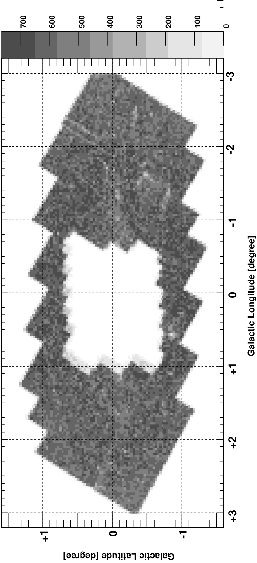
Figure 1: A source density map for stars matched between the IRSF/SIRIUS catalog and the GLMIIC. The bins are $0\fdg 032\times 0\fdg 032$, and star count density is given in unit of $[1000\mathrm{deg}^{-2})]$.

Fig. 2 shows one of the star counts of $0\fdg 2\times 0\fdg 2$ fields for IRSF/SIRIUS, 2MASS, and SST/IRAC. Clear peaks of RC stars are seen in the star counts of IRSF/SIRIUS (indicated by arrows), but not seen in those of 2MASS and SST/IRAC. From the limiting magnitudes obtained by GLIMPSE I (Benjamin et al., 2003), we expected that RC peaks would be detected at least in the [3.6] and [4.5] bands, but source confusion might affect the detection limit of these bands.

To make CMDs involving the SST/IRAC bands when we use the “RC method” following Nishiyama et al. (2006), we need to find stars that are detected in the SST/IRAC bands. Here, we use the upper RGB stars to derive the reddening. We can use the IRSF/SIRIUS $K_{S}$ magnitudes of the RC stars for the derivation of extinction. Assuming that the RC stars and the upper RGB stars are similarly distributed in space with their centers at the GC, we will be able to determine in the CMD the extinction (from RC magnitude shift) and the reddening (from RGB color shift) of a line of sight toward the GC. By plotting the apparent magnitude of the RC stars and the color excess of the RGB of each small field, we obtain a straight line with the slope equal to the total to selective extinction ratio $A_{K_{S}}/E_{K_{S}-\lambda}$ for the SST/IRAC bands.

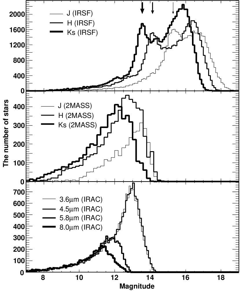
Figure 2: Star counts in the $J,H$ and $K_{S}$ bands from IRSF/SIRIUS (top) and 2MASS (middle), and in the [3.6], [4.5], [5.8], and [8.0] bands from SST/IRAC for one of the fields ($l,b=+0\fdg 9,-0\fdg 9$) towards the GC. Peaks of RC stars can be found only in the top panel, and are indicated by arrows.

As a first step in our analysis, we divided the survey area (Fig. 1) into fields of $0\fdg 2\times 0\fdg 2$. We then made a $K_{S}$-band luminosity function (LF) for each field. A sample of the LFs is shown in Fig. 3, top left panel. A clear peak of RC stars can be found at $K_{S}\sim 14$ mag. We determined the $K_{S}$ peak magnitude (${K_{S}}_{RC}$) by fitting with the Gaussian function (thick line on the LF in Fig. 3).

Figure 3: $K_{S}$-band luminosity function (top left panel) and $K_{S}$ versus $K_{S}-[4.5]$ CMD (top right panel) for one of the fields (centered at $l=-0\fdg 3,b=-0\fdg 7$). The mean $K_{S}-[4.5]$ colors of stars in the dashed rectangles are shown by open circles. By fitting the mean colors, we can determine the RGB slope for this field. Bottom left panel : $K_{S}-[4.5]$ histograms of stars at $13.0<K_{S}<13.5$, which is shown by the bottom rectangle in the top right panel. The histogram is fitted with the Gaussian function to obtain the mean of color. Bottom right panel : Histogram of (RGB slope)^-1 in the $K_{S}$ versus $K_{S}-[4.5]$ CMDs of the fields.

Figure 4: $K_{S}$ versus $K_{S}-\lambda$ CMDs of one field (centered at $l=-0\fdg 3,b=-0\fdg 7$) for $\lambda=[3.6]$ (top left), [4.5] (top right), [5.8] (bottom left), and [8.0] (bottom right).

Second, to determine the color of the RGB, we made $K_{S}$ versus $K_{S}-\lambda$ CMDs for each field and IRAC band. CMDs of one of the fields are shown in Fig. 4 (see also Fig. 3, top right panel for $\lambda=4.5~{}\mu$m). Third, we determined the RGB slope for each field and each IRAC band on the assumption that the RGB can be fitted by a linear function. To do this, we divided $K_{S}$ magnitude of stars on the RGB into bins of equal (0.5 mag) size, which is represented in the top right panel, Fig. 3 by dashed rectangles. Then we calculated the mean of $K_{S}-\lambda$ color of stars in each bin, by fitting the color histogram with the Gaussian function (the bottom left panel in Fig. 3). The bins near the limiting magnitudes and those without enough number of stars were excluded. The mean $K_{S}-[4.5]$ colors for the bins are shown by open circles in the CMD (the top right panel). The RGB slope for each field was obtained from the least-squares fit of the mean $K_{S}-\lambda$ colors with two free parameters: slope and intercept (thick line in the top right panel). The magnitude ranges seem to be wide enough to determine the fairly linear part of the RGB, and narrow enough to exclude both the brighter asymptotic giant branch stars and the fainter RC stars, in these CMDs. We did not find a correlation between the RGB slopes and extinction for each field.

Fourth, we calculated the mean of the RGB slopes in all the IRAC bands. The histogram of the (slopes)^-1 in the $K_{S}$ versus $K_{S}-[4.5]$ CMDs is shown in the bottom right panel. The means of the RGB slopes were then obtained by fitting the histograms with the Gaussian function (the bottom right panel in Fig. 3), as 33.6, 17.9, $-24.6$, and $-19.1$, for the [3.6], [4.5], [5.8], and [8.0] bands, respectively.

Fifth, the color of the RGB in each field was determined assuming that the RGBs in all the fields have the same slope as that obtained in the third and fourth steps (the mean of the RGB slope). The mean $K_{S}-\lambda$ color for each field was determined by a one-parameter (i.e., intercept) least-squares fit with the result expressed as the color the RGB stars would have at the magnitude of the RC stars. Because of the assumption of constant slope, what was actually measured is the color at the centroid of the RGB color-magnitude distribution. The coordinate ($K_{S}-\lambda,{K_{S}}_{RC}$) is the indication of reddening and extinction of each field although RC stars are undetected in the GLIMPSE II catalog (and also in the 2MASS catalog).

4 Results

Fig. 5 (a)-(d) shows the $K_{S}$ magnitude of the RC peak ${K_{S}}_{RC}$ and the $(K_{S}-\lambda)$ color of the RGB of each field in $K_{S}$ versus $K_{S}-\lambda$ CMDs. Error bars on y-axes show uncertainty in RC peak determination, and those on x-axes come from uncertainty of intercepts when the least-squares fit is adopted for the mean $K_{S}-\lambda$ colors. These errors seem to be underestimated because the dispersion of the data points is large compared with the error bars. Hence we estimated the slopes $A_{K_{S}}/E_{K_{S}-\lambda}$ and their errors by applying a least-squares linear fit with $\chi^{2}$ minimization under the assumption that the errors are all equal. We show the linear fits applied to the data points in Fig. 5, and the resultant slopes and their errors are listed in Table 1.

Figure 5: (a)-(d): Distribution of ${K_{S}}_{\mathrm{SIRIUS}}$ magnitudes of a RC peak and ${K_{S}}_{\mathrm{SIRIUS}}-\lambda$ colors of RGB in the $0\fdg 2\times 0\fdg 2$ fields for the [3.6] (a), [4.5] (b), [5.8] (c), and [8.0] (d) IRAC bands.

Figure 6: (a),(b): Distribution of ${K_{S}}_{\mathrm{SIRIUS}}$ magnitudes of a RC peak and $\lambda-{K_{S}}_{\mathrm{SIRIUS}}$ colors of RGB in the $0\fdg 2\times 0\fdg 2$ fields for the 2MASS $J$ (a), and $H$ (b) bands. (c): Distribution of ${K_{S}}_{\mathrm{2MASS}}-{K_{S}}_{\mathrm{SIRIUS}}$ colors of RGB and ${K_{S}}_{\mathrm{SIRIUS}}$ magnitudes of a RC peak in the $0\fdg 2\times 0\fdg 2$ fields. To avoid an infinite value of a linear fitting, x- and y-axes were interchanged compared to (a) and (b).

The same procedure described in the previous section was applied to 2MASS point sources in the $J$, $H$ and $K_{S}$ bands, which are included in the GLMIIC. Fig. 6 show the $K_{S}$ magnitude of the RC peak and the relative ${\lambda}_{\mathrm{2MASS}}-K_{S}$ color of the RGB in $K_{S}$ versus ${\lambda}_{\mathrm{2MASS}}-K_{S}$ CMDs. The dependence of ${K_{S}}_{\mathrm{2MASS}}-K_{S}$ on $K_{S}$ is very small; hence the same plot in a CMD was made for $K_{S}$ and ${K_{S}}_{\mathrm{2MASS}}$, but the x- and y-axes were interchanged to avoid an infinite value of the slope (see Fig. 6). The resultant slopes $A_{K_{S}}/E_{\lambda_{\mathrm{2MASS}}-K_{S}}$ are also summarized in Table 1.

The uncertainty of the RGB slopes is an error source of this method. Hence the fifth step described in §3 was carried out with different RGB slopes, which are $1\sigma$ larger and smaller than those previously used. Here $\sigma$ was obtained when the histograms of (slope)^-1 are fitted with the Gaussian function. The changes of $A_{K_{S}}/E_{K_{S}-\lambda}$ are only less than a few % in the IRAC bands, although those in the 2MASS bands are $2-5$%.

The ratios of total to selective extinction $A_{K_{S}}/E_{K_{S}-\lambda}=A_{K_{S}}/(A_{K_{S}}-A_{\lambda})$ provide us with the ratios of absolute extinction $A_{K_{S}}:A_{\lambda}$ for the IRAC bands. Table 1 presents the extinction ratios $A_{\lambda}/A_{K_{S}}$, which are directly provided by $A_{K_{S}}/E_{K_{S}-\lambda}$. We obtain the wavelength dependence of extinction between $K_{S}$ and IRAC bands, $A_{K_{S}}:A_{[3.6]}:A_{[4.5]}:A_{[5.8]}:A_{[8.0]}=1:0.50:0.39:0.36:0.43$.

We also obtain the extinction ratio in the $J$, $H$ and $K_{S}$ bands in the 2MASS system, ${A_{J}}_{\mathrm{2MASS}}:{A_{H}}_{\mathrm{2MASS}}:{A_{K_{S}}}_{\mathrm{2MASS}}=2.86\pm 0.08:1.60\pm 0.04:1$. These are slightly smaller than those obtained for the MKO system, ${A_{J}}:{A_{H}}:{A_{K_{S}}}=3.02\pm 0.04:1.73\pm 0.03:1$ (Nishiyama et al., 2006), but the differences of them are within less than $2\sigma$ and $3\sigma$ for ${A_{J}}_{\mathrm{2MASS}}/{A_{K_{S}}}_{\mathrm{2MASS}}$ and ${A_{H}}_{\mathrm{2MASS}}/{A_{K_{S}}}_{\mathrm{2MASS}}$, respectively.

To examine possible variations of the extinction law, we divided the survey area into quadrants, N$+$ $(+3\arcdeg>l>0\arcdeg,+1\arcdeg>b>0\arcdeg)$, S$+$ $(+3\arcdeg>l>0\arcdeg,0\arcdeg>b>-1\arcdeg)$, N$-$ $(0\arcdeg>l>-3\arcdeg,+1\arcdeg>b>0\arcdeg)$, and S$-$ $(0\arcdeg>l>-3\arcdeg,0\arcdeg>b>-1\arcdeg)$. The ratios $A_{K_{S}}/E_{K_{S}-\lambda}$ in the quadrants are listed in Table 2. We do not find significant deviation of the ratios from that for all the data points, but we find some trends. The ratios in N$-$ tend to have a smaller value, while those in S$-$ have a larger one. These trends, smaller N$-$ and larger S$-$, have been obtained in $A_{K_{S}}/E_{H-K_{S}}$ (Nishiyama et al., 2006), and similar variations in the extinction law seem to be present among the quadrants in the MIR wavebands. We note again that we do not find statistically significant evidence for differing the extinction laws in different lines of sight toward the GC in the IRAC wavebands.

Since most of stars we detected are in the bar structure whose major axis is oriented at $\sim 20\arcdeg-40\arcdeg$ with respect to the Sun-Galactic center line, different average distance of the giants in a given patch of the sky may cause systematic shifts in positions of the RC peaks and the RGB colors on the $K_{S}$ versus $K_{S}-\lambda$ plot. As shown in Nishiyama et al. (2005), mean magnitude of RC stars weakly depends on the Galactic longitude. However, for changing the ratios of total to selective extinction $A_{K_{S}}/E_{K_{S}-\lambda}$, it is required that the distance to the stars needs to be highly correlated with the reddening. Such correlation seems to be unlikely to exist. A good test for the existence of this systematic error is to compare the ratios $A_{K_{S}}/E_{K_{S}-\lambda}$ for the quadrants, because the error should be reduced in smaller regions due to smaller difference of the distance. As described above, we found insignificant deviation of $A_{K_{S}}/E_{K_{S}-\lambda}$ for the quadrants, and very small difference between the ratios for all the survey area and the weighted mean for the quadrants (see Table 2), suggesting very small systematic shifts on the $K_{S}$ versus $K_{S}-\lambda$ plots due to the difference of the distance.

To confirm that the current method using the RGB and RC stars in deriving the total to selective extinction ratios is consistent with the Nishiyama et al. (2006) method using only the RC stars, we re-analyzed the Nishiyama et al. (2006) data using the RGB and RC stars. The resultant ratios are $A_{K_{S}}/E_{H-K_{S}}=1.46\pm 0.03$ and $A_{K_{S}}/E_{J-K_{S}}=0.499\pm 0.018$, quite consistent with the previously derived ratios $1.44\pm 0.01,0.494\pm 0.006$ in Nishiyama et al. (2006). Therefore, the use of RGB colors does not affect the results.

Table 1: The wavelength dependence of the interstellar extinction in the IRSF/SIRIUS ($J,H,K_{S}$; similar to the MKO filter system), SST/IRAC ([3.6],[4.5],[5.8],[8.0]) and 2MASS ($J_{\mathrm{2MASS}},H_{\mathrm{2MASS}},{K_{S}}_{\mathrm{2MASS}}$) bands.

band	wavelength [$\mu$m]	$A_{K_{S}}/E_{K_{S}-\lambda}$	$A_{\lambda}/A_{K_{S}}$
$J$	1.25	–	$3.02\pm 0.04$
$H$	1.63	–	$1.73\pm 0.03$
$K_{S}$	2.14	–	$1.0$
$[3.6]$	3.545	$2.01\pm 0.04$	$0.50\pm 0.01$
$[4.5]$	4.442	$1.64\pm 0.02$	$0.39\pm 0.01$
$[5.8]$	5.675	$1.56\pm 0.03$	$0.36\pm 0.01$
$[8.0]$	7.760	$1.74\pm 0.04$	$0.43\pm 0.01$
$J_{\mathrm{2MASS}}$	1.240	$-0.528\pm 0.015$	$2.89\pm 0.08$
$H_{\mathrm{2MASS}}$	1.664	$-1.61\pm 0.04$	$1.62\pm 0.04$
${K_{S}}_{\mathrm{2MASS}}$	2.164	$-(0.012\pm 0.002)^{-1}$	$1.012\pm 0.002$

Table 2: The $A_{K_{S}}/E_{K_{S}-\lambda}$ ($A_{K_{S}}/E_{\lambda-K_{S}}$ for the 2MASS bands) for all the survey area, four quadrants, and their weighted mean

band	all data points	N$+$	S$+$	N$-$	S$-$	weighted mean
$[3.6]$	$2.01\pm 0.04$	$2.01\pm 0.07$	$2.03\pm 0.09$	$1.85\pm 0.06$	$2.05\pm 0.09$	$1.96\pm 0.04$
$[4.5]$	$1.64\pm 0.02$	$1.62\pm 0.04$	$1.60\pm 0.05$	$1.59\pm 0.06$	$1.69\pm 0.07$	$1.62\pm 0.02$
$[5.8]$	$1.56\pm 0.03$	$1.56\pm 0.04$	$1.52\pm 0.05$	$1.44\pm 0.04$	$1.64\pm 0.07$	$1.52\pm 0.03$
$[8.0]$	$1.74\pm 0.04$	$1.82\pm 0.06$	$1.67\pm 0.07$	$1.80\pm 0.08$	$1.83\pm 0.09$	$1.77\pm 0.04$
$J_{\mathrm{2M}}$	$0.528\pm 0.015$	$0.497\pm 0.029$	$0.534\pm 0.065$	$0.494\pm 0.021$	$0.587\pm 0.041$	$0.510\pm 0.016$
$H_{\mathrm{2M}}$	$1.61\pm 0.04$	$1.64\pm 0.05$	$1.54\pm 0.08$	$1.48\pm 0.07$	$1.63\pm 0.10$	$1.58\pm 0.04$

5 Discussion

5.1 Comparison of Wavelength Dependence of Extinction with Previous Studies toward the GC

Fig. 7 shows the derived $A_{\lambda}/A_{K_{S}}$ toward the GC (this study; Rieke & Lebofsky, 1985; Lutz, 1999; Jiang et al., 2006). A simple power law of $A_{\lambda}\propto\lambda^{-1.75}$ is also represented. Before the observations by using ISO/SWS, the wavelength dependence of interstellar extinction in the near- to mid-infrared wavelength range (1 - 6 $\mu$m) was thought to be represented by a power law and to be “universal” (Draine, 1989). However, the observation of HII regions around Sgr A* by using ISO/SWS shed serious doubt on a simple power law, and recent observations toward star forming regions with SST/IRAC show clear discontinuity of the power law, preferring flatter extinction toward longer wavelengths.

Analysis of the spectrum of the GC obtained with ISO/SWS revealed an extinction law characterized by a relatively flat behavior at 3 - 8 $\mu$m (Lutz et al., 1996). The extinction measurements were improved by Lutz (1999, open diamonds in Fig. 7), which reinforce the previous flat extinction. In Fig. 7, their $A_{\lambda}/A_{V}$ is converted to $A_{\lambda}/A_{K_{S}}$ by assuming a $\lambda^{-1.99}$ extinction law (Nishiyama et al., 2006) from the $K_{S}$ wavelength to their $\lambda=2.625~{}\mu$m point. Fig. 7 shows that the extinction law derived by Lutz (1999) is very similar to those presented in this work, but discrepancy is slightly large in the [4.5] and [5.8] bands. Some of the discrepancies in $\sim 3-6~{}\mu$m wavelength between Lutz (1999) and our results may be explained by large absorption features observed toward the Sgr A*. Chiar et al. (2000) analysed spectra (2.4 - 13 $\mu$m) toward the Sgr A* and two sources in the Quintuplet cluster, and discussed composition of dust along the lines of sight to them. We can see a deep and broad absorption feature around $\sim 6~{}\mu$m toward the GC for which Chiar et al. (2000) proposed ice mixtures (H₂O:NH₃:CO₂) and HCOOH. A deep absorption feature of H₂O ice at 3 $\mu$m was also detected. The same spectrum was used for Lutz (1999), and thus their higher extinction at 3.0392, 3.2970, and 5.9082 $\mu$m can be attributed to the ice along the line of sight. In contrast, a relatively shallow and narrow absorption was observed for the sources in the Quintuplet cluster. Although it is still unclear how deep and broad the features are along the other lines of sight in the GC region, and two of the higher data points (4.3765 and 5.1287 $\mu$m) cannot be attributed to such absorption features, if the deep and broad absorption features at $\sim$ 3 and 6 $\mu$m are characteristic to only Sgr A* and its immediate vicinity, some of the discrepancies can be naturally explained.

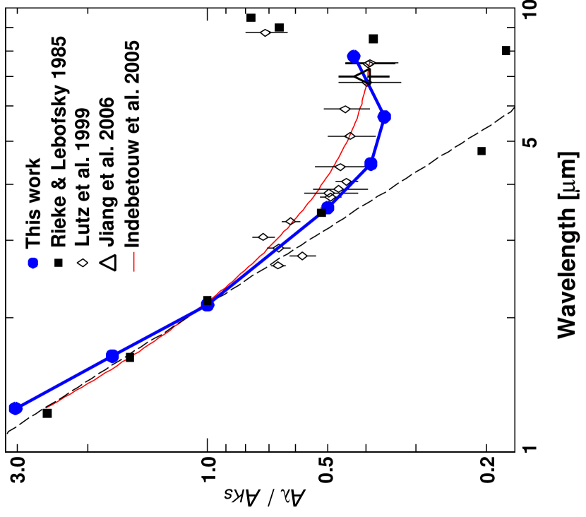
Figure 7: The wavelength dependence of extinction ($A_{\lambda}/A_{K_{S}}$) toward the Galactic center region. The ratios derived by this study (filled blue circles), Lutz (1999, open diamonds), Jiang et al. (2006, open triangle), and Rieke & Lebofsky (1985, filled squares) are represented. Note that in the case of Rieke & Lebofsky (1985), $A_{\lambda}/A_{K}$ instead of $K_{S}$ is represented. A simple power law, $A_{\lambda}\propto\lambda^{-1.75}$ (Draine, 1989) is shown by the dashed line. Although it is not toward the Galactic center, the extinction curve derived by Indebetouw et al. (2005, equation 4) is shown by thin red smooth line for reference.

Fig. 7 shows that the extinction law derived by Rieke & Lebofsky (1985) is much smaller than Lutz (1999) and our results at $>4~{}\mu$m, and the decrease in the 1 - 2.5 $\mu$m range is also very different from our results. Cardelli et al. (1989) fit the data of Rieke & Lebofsky (1985) with a power law $\lambda^{-1.61}$, and it has quite often been referred to as the standard extinction law. However, since Rieke & Lebofsky (1985) laid great emphasis on the determination of $A_{V}/E_{B-V}$ in accordance with the reddening data taken before, $J$ magnitudes of $o$ Sco, Cyg OB2 No.12, and only two stars near the Galactic center were measured with relatively large uncertainties in the color excesses mainly due to the assumed errors in intrinsic colors of these stars. Therefore, the color excesses they determined $E_{V-J}/E_{B-V}=2.19\pm 0.04$ and $E_{V-H}/E_{B-V}=2.55\pm 0.02$ on the assumption of $E_{V-K}/E_{B-V}=2.744$ might be in fact compatible with the current results if we allow for these uncertainties.

The extinction ratios toward the GC in the $J$, $H$ and $K_{S}$ bands in the 2MASS system are consistent with the IRSF/SIRIUS results, as shown in Table 1. These ratios are plotted in Fig. 8, and are consistent with a power law $A_{\lambda}\propto\lambda^{-2.0}$, together with the Nishiyama et al. (2006) results. Therefore, it is established that the interstellar extinction toward the GC in the range of $J$, $H$ and $K_{S}$ bands is well fit by a steep power law of $\lambda^{-2.0}$, not $\lambda^{-1.6}$. Of course, the power law is only an approximation. Since 1) the extinction shows positive deviation from the power law as the wavelength increases to $>3~{}\mu$m as we see above, and 2) a number of dust grain models (e.g., Weingartner & Draine, 2001; Dwek, 2004; Voshchinnikov et al., 2006) predict such positive deviation, it is possible that the power index changes in the $J$, $H$, and $K_{S}$ wavelength range.

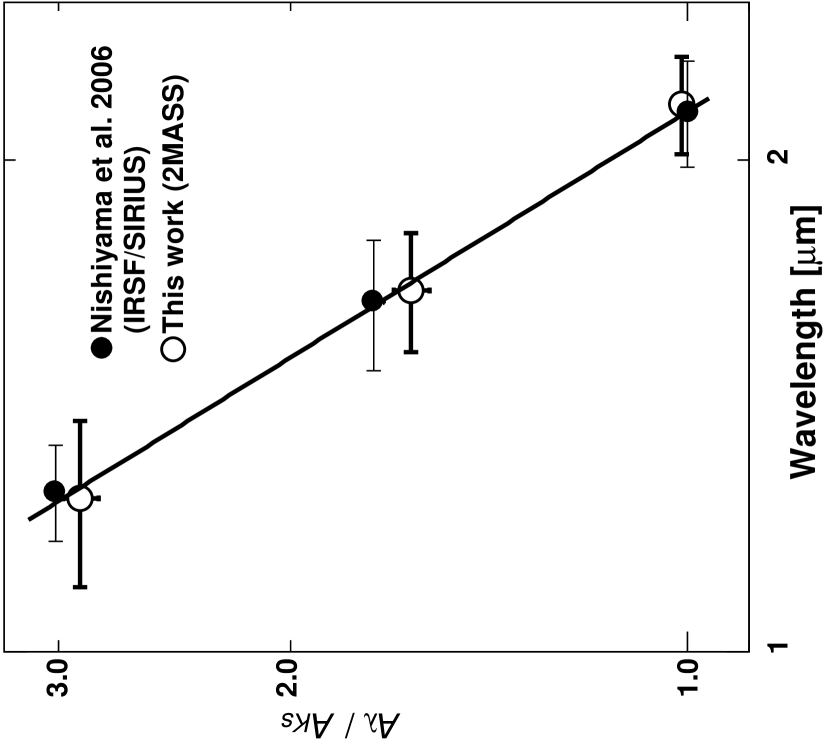
Figure 8: The wavelength dependence of extinction ($A_{\lambda}/A_{K_{S}}$) in the $J$, $H$, and $K_{S}$ bands toward the GC. The results of Nishiyama et al. (2006) in the MKO system are presented by filled circles, and that in the 2MASS system by open circles. A simple power law $A_{\lambda}\propto\lambda^{-2.00}$ fitted to all these points is shown by the straight line. Horizontal bars indicate the filter widths.

5.2 Comparison in the Ratios of Color Excesses

A number of authors obtained the ratios of color excesses first, and then derived the wavelength dependence $A_{\lambda}/A_{K_{S}}$ of the interstellar extinction. However, the assumed ratio $A_{H}/A_{K_{S}}$ leads to a quite different wavelength dependence, as is evident from the equation (2) and was already pointed out by Nishiyama et al. (2006) and Flaherty et al. (2007). Therefore, we convert our $A_{\lambda}/A_{K_{S}}$ to the ratios of color excesses and compare them with the previous results (Fig. 9). This process causes larger errors because of the error propagation, but not any uncertainty at all due to assumption of an unknown parameter as in the inverse procedure.

Flaherty et al. (2007) and Román-Zúñiga et al. (2007) obtained $E_{\lambda-K_{S}}/E_{H-K_{S}}$ (or its reciprocal) from the slopes of the distributions of stars in color-color diagrams. Indebetouw et al. (2005) measured the color excess ratios $E_{\lambda-K_{S}}/E_{J-K_{S}}$, but $E_{\lambda-K_{S}}/E_{H-K_{S}}$ was derived from color-color diagrams (open squares) by Flaherty et al. (2007, see their Table 2) using the same data sets of Indebetouw et al. (2005) and the same method as used in Flaherty et al. (2007). Thus, direct comparison of the wavelength dependence of extinction is possible in color-excess ratios. In Fig. 9, the color-excess ratios $E_{\lambda-K_{S}}/E_{H-K_{S}}$ are plotted against $\lambda^{-1}$ following the convention to compare with scattering calculation.

Differences in $E_{\lambda-K_{S}}/E_{H-K_{S}}$ seem to exist between the star forming regions and the diffuse interstellar medium. The ratios toward the star forming dense core (Román-Zúñiga et al., 2007) and the nearby star forming regions (Flaherty et al., 2007) are very similar, and are in very good agreement within their errors. As indicated by Flaherty et al. (2007), we can find a systematic separation of the ratio toward the off-cloud regions (Indebetouw et al., 2005) from toward the star forming regions. The ratios obtained in this study (calculated from $A_{\lambda}/A_{K_{S}}$) tend to have lower values than those for star forming regions, in the three bands but [8.0]. The higher extinction in the [8.0] band in the direction of the GC than that toward $l=284\arcdeg$ (Indebetouw et al., 2005) is consistent with the claim that the GC line of sight has larger silicate absorption relative to $A_{V}$ (larger $\tau_{9.7}/A_{V}$; Roche & Aitken, 1985) than other lines of sight (see also Table 1, Draine, 2003). A separation between the extinction laws for molecular clouds and for the diffuse interstellar medium in the color excess ratios $E_{[3.6]-[4.5]}/E_{[4.5]-[5.8]}$ suggested by Flaherty et al. (2007) is not confirmed in Fig. 9 due to the large uncertainties. However, we can find a clear difference in $E_{\lambda-K_{S}}/E_{H-K_{S}}$ between the star forming regions and the off-cloud regions including toward the GC.

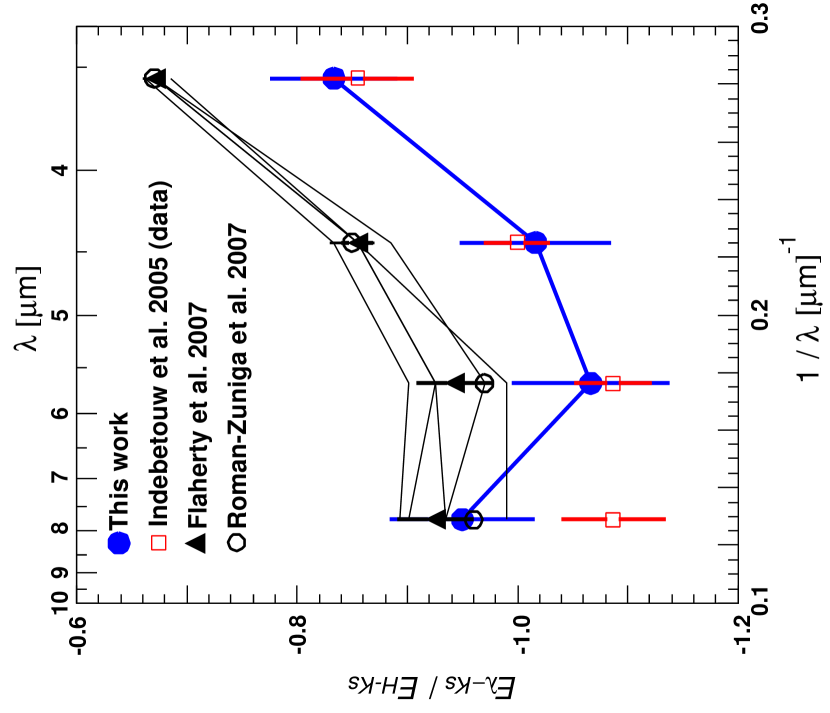
Figure 9: Color excess ratio $E_{\lambda-K_{S}}/E_{H-K_{S}}$ versus wavelength diagram in the IRAC bands derived by this study (blue filled circles) and Román-Zúñiga et al. (2007, open circles). The ratios derived by Flaherty et al. (2007) for five star-forming regions (solid lines) and their weighted mean (filled triangles) are also plotted. Here all the $H$ and $K_{S}$ bands are those of the 2MASS survey. The ratio $E_{\lambda-K_{S}}/E_{H-K_{S}}$ was not directly measured by Indebetouw et al. (2005), but Flaherty et al. (2007) directly determined $E_{\lambda-K_{S}}/E_{H-K_{S}}$ for the same data sets of Indebetouw et al. (2005), and this is shown by red open squares. So the data points shown in this figure, except ours (blue circles), are directly measured from color-color diagrams. Only ours are converted from $A_{\lambda}/A_{K_{S}}$ to $E_{\lambda-K_{S}}/E_{H-K_{S}}$.

5.3 Absolute Extinction Ratios in Different Lines of Sight

Absolute extinction has only been measured for the GC, and comparison with other lines of sight requires an assumption of at least one extinction ratio (e.g., $A_{H}/A_{K_{S}}$). Here, we assume a single power law for the interstellar extinction instead, and try to derive its index. Flaherty et al. (2007) measured $E_{J-K_{S}}/E_{H-K_{S}}$ in NGC 2024/2023, NGC 2068/2071, and Serpens, which are $3.00\pm 0.04$, $2.98\pm 0.03$, and $3.05\pm 0.04$, respectively. They also derived the ratio for the $l=284\arcdeg$ region (Indebetouw et al., 2005) with the result of $3.07\pm 0.04$, pointing that no significant variation seems to exist in the near-infrared extinction law through these molecular clouds and through the diffuse interstellar medium. Assuming the effective wavelengths of the 2MASS observations to be 1.240, 1.664, and 2.164 $\mu$m (Indebetouw et al., 2005) and that the extinction is approximated by a power law, we can derive the power law index for these lines of sight. The resultant indices are from $-2.04$ to $-2.18$. Thus, the interstellar extinction for all these lines of sight seems to be fitted by a single power law of $A_{\lambda}\propto\lambda^{-2.0}$, which is the same as that in the GC, very well in the $J$, $H$, and $K_{S}$ wavelength range. However, the extinction law derived by Indebetouw et al. (2005) decreases much more slowly to the longer wavelength (slower than $\lambda^{-1.7}$), and nonetheless their data are shown by Flaherty et al. (2007) to have a consistent $E_{J-K_{S}}/E_{H-K_{S}}$ ratio $3.07\pm 0.04$. (Note that Table 1 in Indebetouw et al. (2005) lists smaller $E_{J-K_{S}}/E_{H-K_{S}}$ ratios, possibly because of the difference in the selection criteria of background stars by them and by Flaherty et al. (2007).) Therefore, from the color excess ratios one cannot resolve the degeneracy. Both a steep power law upto the $K_{S}$ band similar to the GC and a much gentler extinction curve are consistent with the color excess ratios. In particular, the frequently employed $JHK_{S}$ color-color diagrams can be quite insensitive to the change in extinction law. Hence, we cannot determine a value of $A_{H}/A_{K_{S}}$ even from a seemingly similar $E_{J-K_{S}}/E_{H-K_{S}}$ values. We further should be cautious, because line-of-sight differences in $E_{J-K_{S}}/E_{H-K_{S}}$ do seem to exist. For example, Naoi et al. (2006) found color excess ratios in $\rho$ Oph and Cha I star-forming regions consistent with that in the GC, but a significantly larger ratio in the Coalsack Globule 2 (Naoi et al., 2007).

It is quite straightforward to determine $A_{\lambda}/A_{K_{S}}$ in this work from the direct measurement of the ratios of total to selective extinction $A_{K_{S}}/E_{K_{S}-\lambda}$. In contrast, to derive $A_{\lambda}/A_{K_{S}}$ in the equation (2) in the color-color method is a difficult and crucial task, which Indebetouw et al. (2005) made from the determination of $A_{H}/A_{K_{S}}$. Since Flaherty et al. (2007) and Román-Zúñiga et al. (2007) did not determine $A_{H}/A_{K_{S}}$, they converted their color excess ratios to $A_{\lambda}/A_{K_{S}}$ using the ratio $A_{H}/A_{K_{S}}=1.55$ derived by Indebetouw et al. (2005). However, there is no clear evidence for universality of $A_{H}/A_{K_{S}}$, and a different $A_{H}/A_{K_{S}}$ leads to a different $A_{\lambda}/A_{K_{S}}$ as described in §5.2, and as also pointed out by Flaherty et al. (2007). The difference is shown in Fig. 10 in which $A_{H}/A_{K_{S}}=1.60$ in addition to $1.55$ is used to derive another set of $A_{\lambda}/A_{K_{S}}$ ratios based on the Flaherty et al. (2007) and Román-Zúñiga et al. (2007) color excess observations.

The ratio of $A_{H}/A_{K_{S}}=1.55$ produces larger separation between the line of sights to molecular cloud and diffuse interstellar medium. The average of the four lines of sight to the star-forming regions studied by Flaherty et al. (2007) and the dark cloud core by Román-Zúñiga et al. (2007) show higher extinction in the IRAC bands than the GC and the $l=284\arcdeg$ diffuse medium (Indebetouw et al., 2005). In contrast, if we assume the ratio of $A_{H}/A_{K_{S}}=1.60$, the molecular-cloud data points shift to the GC and the diffuse interstellar medium, although $A_{H}/A_{K_{S}}\approx 1.69$ is needed to make the results of Flaherty et al. (2007) and Román-Zúñiga et al. (2007) agree with our results. Therefore, if we assume that the near-infrared extinction laws are different in the dense clouds and diffuse clouds, then the difference continues to the mid-infrared, and vice versa. Currently, we do not have sufficient data to distinguish these two possibilities because the measurement of the total to selective extinction is very difficult in the lines of sight other than the GC. However, the difference in $E_{\lambda-K_{S}}/E_{H-K_{S}}$ (see Fig. 9) and the required $A_{H}/A_{K_{S}}$ of $\approx 1.69$ suggest that all of the observational results discussed in this paper cannot be reconciled with a single extinction law.

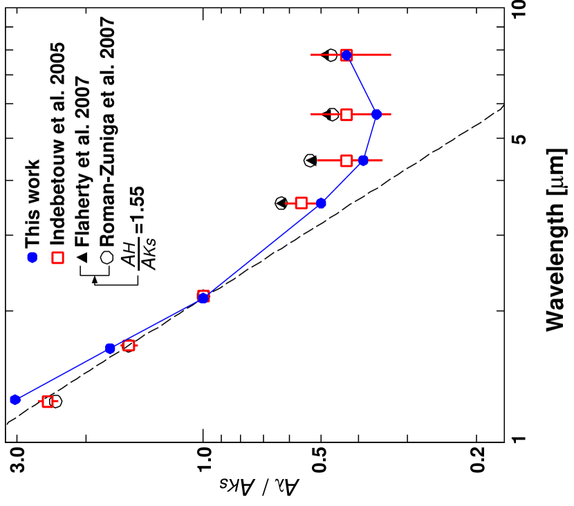
Figure 10: Left : The wavelength dependence of extinction ($A_{\lambda}/A_{K_{S}}$). The blue filled circles (this study) is the extinction law toward the Galactic center, and the red open squares are that for off-cloud regions in the Galactic plane (Indebetouw et al., 2005). Those for star forming regions derived by Flaherty et al. (2007) and Román-Zúñiga et al. (2007) are shown by filled triangles and open circles, respectively, in the assumption of $A_{H}/A_{K_{S}}=1.55$ (Indebetouw et al., 2005). A simple power law, $A_{\lambda}\propto\lambda^{-1.75}$ is shown by the dashed line (Draine, 1989). Right : The same extinction laws derived by this work and Indebetouw et al. (2005) are shown, but those for Flaherty et al. (2007) and Román-Zúñiga et al. (2007) are slightly different due to the different assumption of $A_{H}/A_{K_{S}}=1.60$ corresponding to a steep power law.

6 Conclusion

We have measured the wavelength dependence of interstellar extinction toward the GC in the 1.2 - 8.0 $\mu$m region by combining the IRSF/SIRIUS infrared observations and the 2MASS and SST/IRAC catalogs. The extinction in the wavelength range of $J$, $H$, and $K_{S}$ is well fitted by a power law of steep decrease $A_{\lambda}\propto\lambda^{-2.0}$ toward the GC. Furthermore, the flattening of the extinction from a simple extrapolation toward the longer wavelength of the power law at $\lesssim 3~{}\mu$m has been confirmed. In particular, the extinction has a relatively shallow and broad minimum in the SST/IRAC wavelength range; $A_{[4.5]}$ and $A_{[5.8]}$ are only slightly smaller than 0.4 times $A_{{K}_{S}}$.

This dependence has been derived directly from the observation of reddening in proportion to the $K_{S}$ extinction for the first time involving the SST/IRAC wavebands. In this, the $K_{S}$ magnitudes of RC stars and the $K_{S}-\lambda$ colors of RGB stars serve as a tracer of the reddening vector in the color-magnitude diagrams, and the ratios of total to selective extinction $A_{K_{S}}/E_{K_{S}-\lambda}$ have been obtained by a variant of the “RC method” originated from the variable-extinction method. It is interesting to note that this method is only sensitive to the spatially variable component in the surveyed area; when a star cluster suffers patchy $0.8-1.4$mag extinction from region to region, then the total to selective extinction ratio for the variable $0.6$mag component is derived, but the characteristics of the ubiquitous $0.8$ mag extinction component remain unknown. This can be its strong point because it is not so sensitive to the intrinsic magnitudes and colors of these background stars; on the other hand, the location of the dust grains causing this variable extinction in the long line of sight to the GC is not certain. However, since the silicate absorption seems fairly strong, the dominant grain population probed in this method is probably in the vicinity of the GC. It should be also noted that the assumptions used here are that the RC stars and RGB stars have spatial distributions with their centers in common, and that the reddening of RGB stars can be measured precisely from the shape of upper giant branch.

The wavelength dependence seems to be different among the various lines of sight. In particular, the GC and off-cloud regions show different extinction law from star-forming regions, although the difference is not very large compared to the observational uncertainties. The general behavior of extinction curves, which decreases steeply in the near-infrared, but decreases only slightly beyond the $K_{S}$ band, is an important constraint when dust grain models are discussed.

References

- Benjamin et al. (2003) Benjamin, R. A., et al. 2003, PASP, 115, 953
- Cardelli et al. (1989) Cardelli, J. A., Clayton, G. C., & Mathis, J. S., 1989, ApJ, 345, 245
- Chiar et al. (2000) Chiar, J. E., Tielens, A. G. G. M., Whittet, D. C. B., Schutte, W. A., Boogert, A. C. A., Lutz, D., van Dishoeck, E. F., & Bernstein, M. P. 2000, ApJ, 537, 749
- Draine (1989) Draine, B. T. 1989, in Infrared Spectroscopy in Astronomy, ed. B. H. Kaldeich (ESA SP-290; Paris: ESA), 93
- Draine (2003) Draine, B. T., 2003, ARA&A, 41, 241
- Dutra et al. (2003) Dutra, C. M., Santiago, B. X., Bica, E. L. D., & Barbuy, B. 2003, MNRAS, 338, 253
- Dwek (2004) Dwek, E. 2004, ApJ, 611, L109
- Fazio et al. (2004) Fazio, G. G., et al. 2004, ApJS, 154, 10
- Flaherty et al. (2007) Flaherty, K. M., Pipher, J. L., Megeath, S. T., Winston, E. M., Gutermuth, R. A., Muzerolle, J., Allen, L. E., & Fazio, G. G. 2007, ApJ, 663, 1069
- Frogel et al. (1999) Frogel, J. A., Tiede, G. P., & Kuchinski, L. E. 1999, AJ, 117, 2296
- Indebetouw et al. (2005) Indebetouw, R., et al. 2005, ApJ, 619, 931
- Jiang et al. (2006) Jiang, B. W., Gao, J., Omont, A., Schuller, F., & Simon, G. 2006, A&A, 446, 551
- Krełowski & Papaj (1993) Krełowski, J., & Papaj, J., 1993, PASP, 105, 1209
- Lutz et al. (1996) Lutz, D., et al. 1996, A&A, 315, L269
- Lutz (1999) Lutz, D., 1999, in The Universe as Seen by ISO, ed. P. Cox & M. F. Kessler ( ESA SP-427; Noordwijk: ESA), 623
- Meade et al. (2008) Meade, M. R. et al. 2008, http://www.astro.wisc.edu/sirtf/glimpse2_dataprod_v2.0.pdf
- Nagashima et al. (1999) Nagashima, C., et al. 1999, in Star Formation 1999, ed. T. Nakamoto (Nobeyama : Nobeyama Radio Obs.), 397
- Nagata et al. (1994) Nagata, T., Kobayashi, N., & Sato, S., 1994, ApJ, 423, L113
- Nagayama et al. (2003) Nagayama, T., et al. 2003, Proc. SPIE, 4841, 459
- Naoi et al. (2006) Naoi, T. et al. 2006, ApJ, 640, 373
- Naoi et al. (2007) Naoi, T. et al. 2007, ApJ, 658, 1114
- Nishiyama et al. (2005) Nishiyama, S. et al. 2005, ApJ, 621, L105
- Nishiyama et al. (2006) Nishiyama, S. et al. 2006, ApJ, 638, 839
- Nishiyama et al. (2008) Nishiyama, S., Nagata, T., Tamura, M., Kandori, R., Hatano, H., Sato, S., Sugitani, K. 2008, ApJ, 680, 1174
- Persson et al. (1998) Persson, S. E., Murphy, D. C., Krzeminski, W., Roth, M., & Rieke, M. J. 1998, AJ, 116, 2475
- Rieke & Lebofsky (1985) Rieke, G. H., & Lebofsky, M. J. 1985, ApJ, 288, 618
- Roche & Aitken (1985) Roche, P. F. & Aitken, D. K. 1985, MNRAS, 215, 425
- Román-Zúñiga et al. (2007) Román-Zúñiga, C. G., Lada, C. J., Muench, A., & Alves, J. F. 2007, ApJ, 664, 357
- Schultheis et al. (1999) Schultheis, M. et al. 1999, A&A, 349, L69
- Skrutskie et al. (2006) Skrutskie, M. F., et al. 2006, AJ, 131, 1163
- Stetson (1987) Stetson, P. B., 1987, PASP, 99, 191
- Tiede et al. (1995) Tiede, G. P., Frogel, J. A., & Terndrup, D. M. 1995, AJ, 110, 2788
- Tokunaga et al. (2002) Tokunaga, A. T., Simons, D. A., & Vacca, W. D., 2002, PASP, 114, 180
- Voshchinnikov et al. (2006) Voshchinnikov, N. V., Il’in, V. B., Henning, Th., & Dubkova, D. N. 2006, A&A, 445, 167
- Weingartner & Draine (2001) Weingartner, J. C. & Draine, B. T. 2001 ApJ, 548, 296
- Woźniak & Stanek (1996) Woźniak, P. R., & Stanek, K. Z., 1996, ApJ, 464, 233