Negative conductances of Josephson junctions: Voltage fluctuations and energetics

Abstract

We study a resistively and capacitively shunted Josephson junction, which is driven by a combination of time-periodic and constant currents. Our investigations concern three main problems: (A) The voltage fluctuations across the junction; (B) The quality of transport expressed in terms of the Péclet number; (C) The efficiency of energy transduction from external currents. These issues are discussed in different parameter regimes that lead to: (i) absolute negative conductance; (ii) negative differential conductance, and (iii) normal, Ohmic-like conductance. Conditions for optimal operation of the system are studied.

I Introduction

Transport processes in periodic systems play an important role in a great variety of everyday life phenomena. Two prominent examples are the electric transport in metals providing a prerequisite of modern civilization, and the movement of so-called molecular motors (like kinesin and dynein) along microtubules in biological cells which are of crucial relevance for the functioning of any higher living organism. Josephson junctions belong to the same class of systems being characterized by a spatially periodic structure. In the limiting case of small tunnel contacts the mathematical description of a Josephson junction is identical to that of a Brownian particle moving in a periodic potential. Such models have also frequently been employed under nonequilibrium conditions to describe Brownian ratchets and molecular motors, see Refs hanRev ; motor and references therein. Of particular importance for technological applications are ’rocked’ thermal Brownian motors operating either in overdamped or underdamped regimes, e.g. see in Ref. rocked . The majority of papers on transport in periodic systems are focused on the asymptotic long time behavior of averaged quantities such as the mean velocity of a molecular motor, or the mean voltage drop in a Josephson contact ratchet . The main emphasis of these works lies on formulating and exploring conditions that are necessary for the generation and control of transport, its direction, and magnitude as well as its dependence on system parameters like temperature and external load. Apart from these well investigated questions other important features concerning the quality of transport though have remained unanswered to a large extent. The key to these problems lies in the investigation of the fluctuations about the average asymptotic behavior machuraJPC .

In the present paper we continue our previous studies on anomalous electric transport in driven, resistively and capacitively shunted Josephson junction devices machuraPRL ; aip ; kosturPRB . These investigations were focused on the current-voltage characteristics, in particular on negative conductances. In contrast, in the present paper we investigate the fluctuations of voltage, the diffusion processes of the Cooper pair phase difference across a Josephson junction as well as the energetic performance of such a device.

The paper is organized as follows. In the next section, we briefly describe the Stewart-McCumber model for the dynamics of the voltage across a junction. In Section 3, we study voltage fluctuations, phase difference diffusion, and the efficiency of the device. Conclusions are contained in Section 4.

II Model of resistively and capacitively shunted Josephson junction

The Stewart-McCumber model describes the semi-classical regime of a small (but not ultra small) Josephson junction for which a spatial dependence of characteristics can be neglected. The model contains three additive current contributions: a Cooper pair tunnel current characterized by the critical current $I_{0}$, a normal (Ohmic) current characterized by the normal state resistance $R$ and a displacement current due to the capacitance $C$ of the junction. Thermal fluctuations of the current are taken into account according to the fluctuation-dissipation theorem and satisfy the Nyquist formula associated with the resistance $R$. The quasi-classical dynamics of the phase difference $\phi=\phi(t)$ between the macroscopic wave functions of the Cooper pairs on both sides of the junction is described by the following equation barone ; kautz ,

$$\frac{\hbar}{2e}C\>\ddot{\phi}+\frac{\hbar}{2e}\frac{1}{R}\dot{\phi}+I_{0}\sin(\phi)=I_{d}$$

$$+I_{a}\cos(\Omega t+\varphi_{0})+\xi(t)\;,$$ (1)

where the dot denotes the differentiation with respect to time, $I_{d}$ and $I_{a}$ are the amplitudes of the applied direct (dc) and alternating (ac) currents, respectively, $\Omega$ is the angular frequency and $\varphi_{0}$ defines the initial phase value of the ac-driving. Thermal equilibrium fluctuations are modeled by zero-mean Gaussian white noise $\xi(t)$ with the correlation function $<\xi(t)\xi(s)>=(2k_{B}T/R)\>\delta(t-s)$, where $k_{B}$ is the Boltzmann constant and $T$ is temperature of the system.

The limitations of the Stewart-McCumber model and its range of validity are discussed e.g. in Sec. 2.5 and 2.6 of Ref. kautz . There are various other physical systems that are described by Eq. (II). A typical example is a Brownian particle moving in the spatially periodic potential $U(x)=U(x+L)=-\cos(x)$ of period $L=2\pi$, driven by a time-periodic force and a constant force machuraJPC . In this case, the variable $\phi$ corresponds to the spatial coordinate $x$ of the Brownian particle and ac and dc play the role of periodic driving and a static tilt force, respectively, acting on the particle. Other specific systems are: a pendulum with an applied torque barone , rotating dipoles in external fields Reg2000 ; Coffey , superionic conductors Ful1975 and charge density waves Gru1981 .

It is convenient to transform Eq. (II) to a dimensionless form. We rescale the time $t^{\prime}=\omega_{p}t$, where $\omega_{p}=(1/\hbar)\sqrt{8E_{J}E_{C}}$ is the Josephson plasma frequency expressed by the Josephson coupling energy $E_{J}=(\hbar/2e)I_{0}$ and the charging energy $E_{C}=e^{2}/2C$. Then Eq. (II) takes the form barone ; kautz

$$\frac{d^{2}\phi}{dt^{\prime 2}}+{\gamma}\frac{d\phi}{dt^{\prime}}+\sin(\phi)=i_{0}+i_{1}\cos(\Omega_{1}t^{\prime}+\varphi_{0})$$

$$+\sqrt{2\gamma D}\;\Gamma(t^{\prime}).$$ (2)

The dimensionless damping constant ${\gamma}=1/\omega_{p}RC$ is given by the ratio of two characteristic times: $\tau_{0}=1/\omega_{p}$ and the relaxation time $\tau_{r}=RC$. This damping constant $\gamma$ measures the strength of dissipation. The ac amplitude and angular frequency are $i_{1}=I_{a}/I_{0}$ and $\Omega_{1}=\Omega\tau_{0}=\Omega/\omega_{p}$, respectively. The rescaled dc strength reads $i_{0}=I_{d}/I_{0}$. The rescaled zero-mean Gaussian white noise $\Gamma(t^{\prime})$ possesses the auto-correlation function $\langle\Gamma(t^{\prime})\Gamma(u)\rangle=\delta(t^{\prime}-u)$, and the noise intensity $D=k_{B}T/E_{J}$ is given as the ratio of two energies, the thermal energy and the Josephson coupling energy (corresponding to the barrier height).

Because Eq. (II) is equivalent to a set of three autonomous first order ordinary differential equations, the phase space of (II) is three-dimensional. For vanishing diffusion constant, $D=0$, the system becomes deterministic. The resulting deterministic nonlinear dynamics ($D=0$) exhibits a very rich behavior ranging from periodic to quasi-periodic and chaotic solutions in the asymptotic long time limit. Moreover, there are regions in parameter space where several attractors coexist. In the presence of small noise these attractors still dominate the dynamics in the sense that most of the time the trajectory stays close to one of these attractors. Only rarely, transitions between the attractors take place. So, the locally stable states of the noiseless dynamics become metastable states in the presence of weak noise. Apart from that, the presence of noise may also let the system come close to deterministic unstable orbits which it may follow for quite some time.

Strictly speaking, the deterministic regime $D=0$ is only reached in the limit of zero temperature for which quantum effects become relevant. These are not taken into account in the classical Langevin equation (II). However, for sufficiently large Josephson junctions a region of low temperatures exists for which both thermal and classical fluctuations can be neglected on those time scales that are experimentally relevant.

The averaged transport behavior is completely determined by the current–voltage characteristic, i.e. the functional dependence of the averaged voltage on the applied dc–strength in the asymptotic limit of large times when all transient phenomena have died out. To obtain this current–voltage characteristic, we numerically simulated $10^{3}$ solutions of Eq. (II) from which we estimated the stationary dimensionless voltage defined as

$$v=\langle\dot{\phi}(t^{\prime})\rangle,$$ (3)

where the brackets denote averages (i) over the initial conditions $(\phi(0),\dot{\phi}(0),\varphi_{0})$ according to a uniform distribution on the cube $\{\phi(0)\in[0,2\pi],\dot{\phi}(0)\in[-2,2],\varphi_{0}\in[0,2\pi]\}$, (ii) over realizations of thermal noise $\Gamma(t^{\prime})$ and (iii) a temporal average over one cycle period of the external ac-driving once the result of the first two averages have evolved into a periodic function of time. The stationary physical voltage is then expressed as

$$V=\frac{\hbar\omega_{p}}{2e}\;v.$$ (4)

For a vanishing dc–strength, $i_{0}=0$, also the average voltage must vanish because under this condition Eq. (2) as well as the probability distribution with respect to which the average is performed are invariant under the transformation $(\phi,\varphi_{0})\to(-\phi,\varphi_{0}+\pi)$. For non-zero currents $i_{0}\neq 0$, this symmetry is broken and the averaged voltage can take non-zero values, which typically assume the same sign as the bias current $i_{0}$. Apart from this “standard” behavior, a Josephson junction may also exhibit other more exotic features, such as absolute negative conductance (ANC) machuraPRL ; aip , negative differential conductance (NDC), negative–valued nonlinear conductance (NNC) and reentrant effects into states of negative conductance aip ; kosturPRB . In mechanical, particle-like motion terms, these exotic transport patterns correspond to different forms of negative mobility of a Brownian particle.

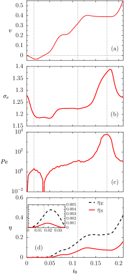
Figure 1: (color online) Various performance measures of a Josephson junction in dependence of the dc–strength are compared. In panel (a) the stationary voltage $v$ defined in Eq. (3) is depicted while panels (b), (c) and (d) display the standard deviation $\sigma_{v}$ as a measure the voltage fluctuations, cf. eq. (5), the Péclet number Pe (Eq. (11)) and the two efficiency measures $\eta_{E}$ (Eq. 7) and $\eta_{S}$ (Eq. 9), respectively. The remaining system’s parameters are: the thermal noise intensity $D=0.001$, ac driving frequency $\Omega=0.78$, ac driving amplitude $i_{1}=0.732$ and damping constant $\gamma=0.143$. Three thin vertical lines mark the three dc–strengths $i_{0}=0.0159$ (regime of absolute negative conductance), $i_{0}=0.1114$ (Ohmic-like regime, chaotic regime, large diffusion, relatively small current fluctuations), $i_{0}=0.175$ (regime of negative differential conductance, very regular motion, small diffusion but relatively large current fluctuations). For corresponding trajectories and phase portraits see Figs. 2, 3 and 4.

III Transport characteristics

Apart from the averaged stationary velocity $v$, which presents the basic transport measure, there are other quantities that characterize the random deviations of the voltage about its average $v$ at large times such as the voltage variance

$$\sigma_{v}^{2}=\langle\dot{\phi}^{2}\rangle-\langle\dot{\phi}\rangle^{2}.$$ (5)

Here the average is performed with respect to the same probability distribution as for $v$ in Eq. (3). This variance determines the range

$$v(t^{\prime})\in\left(v-\sigma_{v},v+\sigma_{v}\right)$$ (6)

of the dimensionless voltage $v(t^{\prime})=\dot{\phi}(t^{\prime})$ in which its actual value is typically found. Therefore the voltage may assume the opposite sign to the average voltage $v$ if $\sigma_{v}>v$.

In order to quantify the effectiveness of a device in terms of the power output at a given input, several measures have been proposed in the literature bier ; Sekimoto2000 ; Suzuki2003 ; wang ; machuraPRE ; rozen . Here we discuss two of them, which yield consistent results. For the systems described by Eq. (II), the efficiency of energy conversion is defined as the ratio of the power $P=i_{0}v$ done against an external bias $i_{0}$ and the input power $P_{in}$ sintes ; physA ,

$$\eta_{E}=\frac{|i_{0}v|}{P_{in}},$$ (7)

where $P_{in}$ is the total ac and dc power supplied to the system. It is given by machuraPRE

$$P_{in}=\gamma[v^{2}+\sigma_{v}^{2}-D]=\gamma[\langle\dot{\phi}^{2}\rangle-D].$$ (8)

This relation follows from an energy balance of the underlying equation of motion (II). Further, the Stokes efficiency is given by the relation wang

$$\eta_{S}=\frac{i_{\gamma}v}{P_{in}}=\frac{\gamma v^{2}}{P_{in}}=\frac{v^{2}}{v^{2}+\sigma_{v}^{2}-D},$$ (9)

where $i_{\gamma}=\gamma v$ denotes the Ohmic current, cf. Eq. (II). In contrast to the definition of the efficiency of energy conversion $\eta_{E}$, the definition of the Stokes efficiency $\eta_{S}$ does not contain the damping constant $\gamma$. We note that a decrease of the voltage variance $\sigma_{v}^{2}$ leads to a smaller input power and hence to an increase of the energetic efficiency.

Another quantity that characterizes the effectiveness of transport is the effective diffusion coefficient of the phase difference $\phi(t)$, describing the spreading of trajectories and fluctuations around the average phases. It is defined as follows

$$D_{\phi}=\lim_{t\rightarrow\infty}\frac{\langle\phi^{2}(t)\rangle-\langle\phi(t)\rangle^{2}}{2t}.$$ (10)

The coefficient $D_{\phi}$ can also be introduced via a generalized Green-Kubo relation machuraJPC . Intuitively, the diffusion coefficient is small and the transport is more effective if the stationary voltage is large and the spread of trajectories is small. The ratio $D_{\phi}/2\pi$ can be considered as a velocity characterizing the phase difference diffusion over one period. Its relation to the averaged velocity $v$ of the phase difference determines the dimensionless Péclet number Pe defined as

$$\mbox{Pe}=\frac{2\pi|\langle v\rangle|}{D_{\phi}}.$$ (11)

A large Péclet number indicates a motion of mainly regular nature. If it is small then random or chaotic influences dominate the dynamics.

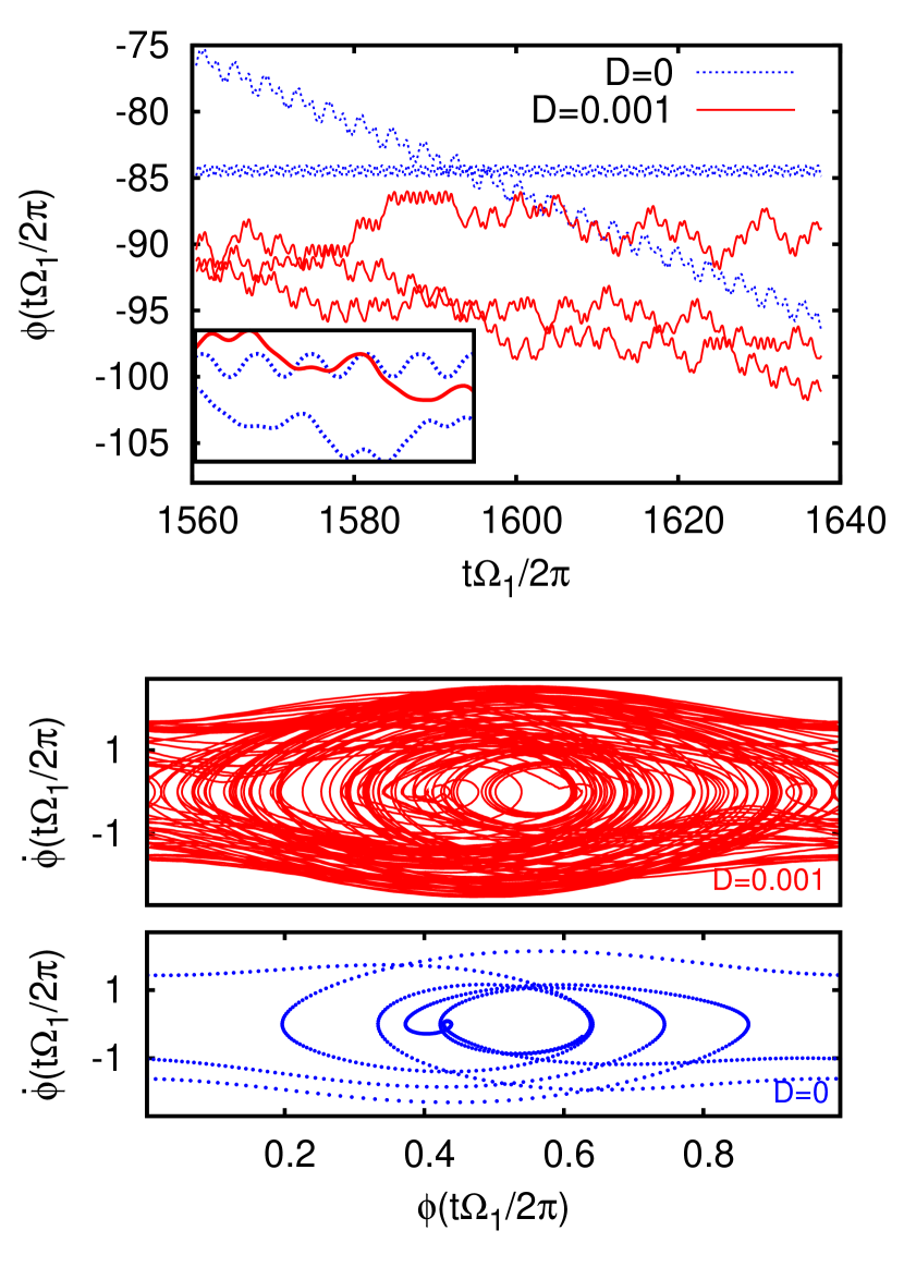
Figure 2: (color online) In the ANC regime at the dc–strength $i_{0}=0.0159$ the deterministic trajectories, $D=0$, (blue dotted lines) for large times (upper panel) approach either a locked solution in one of the wells of the periodic potential or a running solution that proceeds in the negative direction opposite to the positive dc–bias. The remaining parameters are the same as in Fig. 1. The sample trajectories of the Langevin equation (II) (red solid lines), resulting for the noise strength $D=0.001$ and the same other parameters, stay close to either of the deterministic trajectories for some time and then switch to the neighborhood of another trajectory. The inset of the upper panel displays the locked and the running deterministic trajectory and one realization of a stochastic trajectory for five periods of the ac driving. The corresponding phase portraits for the deterministic running solution and the stochastic trajectory are shown in lower panels.

Figure 3: (color online) In the Ohmic like regime at $i_{0}=0.1114$ (other parameters as in the Figs. 1 and 2) the deterministic motion for $D=0$ (blue dotted line) is chaotic in the limit of large times. The phase difference $\phi(t)$ increases on average, hence leading to normal conductance, see the upper panel. In their qualitative appearance the deterministic trajectories are not different from the stochastic trajectories (red solid line) for the noise strength $D=0.001$. The Poincaré map of the deterministic system for the same set of parameters is displayed in the lower panel. This map represents the phase difference modulo $2\pi$ and the corresponding velocity of a single trajectory taken at integer multiples of the ac driving period, see e.g. Strogatz . It reveals the typical features of a strange attractor.

Fig. 1 depicts the main transport characteristics. Panel (a) represents the dependence of the averaged voltage on the dc–strength. It displays ANC for small dc–strengths and NDC for larger dc–values. Fig. 2 of Ref. kosturPRB seemingly exhibits a very similar behavior. The present ac–strength $i_{1}=0.732$ however is somewhat larger than the one chosen in Ref. kosturPRB . As a consequence, the present set of parameters leads to ANC already for $D=0$. The deterministic motion then is governed by two coexisting attractors, a locked and a non–chaotic running solution, see Fig. 2.

In panel (b) of Fig. 1 the standard deviation $\sigma_{v}$ of the voltage is depicted as a function of $i_{0}$. We note that its dependence on the dc–strength is rather complicated and without any immediately obvious relation to the averaged voltage of panel (a). Upon closer inspection, one though observes that the voltage fluctuations undergo rapid changes yielding a large standard deviation in the vicinity of zero bias (at small dc–values) and in the interval where the regime of the NDC appears. In these regimes, the maxima of the standard deviation are found, cf. the inset in the upper panel of Fig. 4, where one can reveal oscillations in the potential well. Upon a further increase of the dc–strength, the voltage fluctuations decrease because the influence of the periodic potential then becomes weaker. Since in this limit oscillations and back–turns of the trajectories become less frequent the standard deviation of the voltage decreases.

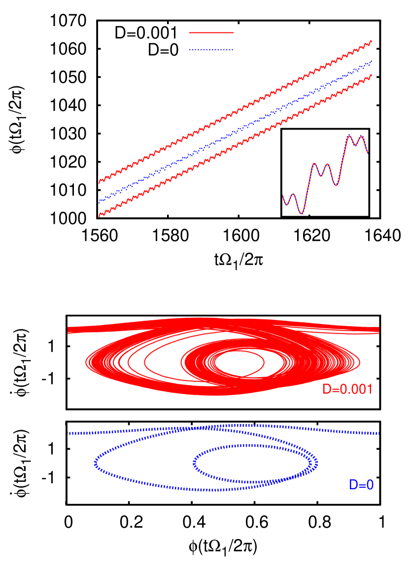
Figure 4: (color online) In the regime of NDC at $i_{0}=0.175$ (all other parameters as in the previous Figs.) the deterministic motion is represented by periodic trajectories (blue dotted lines) running in the positive direction. In this parameter regime the stochastic trajectories at $D=0.001$ (red solid line) stay much closer and for much longer times nearby a deterministic trajectory than in the cases displayed in Figs 2 and 3 (see the magnification in the inset and also compare with the inset of the upper panel of Fig. 3). This explains the small value of the phase diffusion coefficient $D_{\phi}$ in this parameter regime, see also panel (c) of Fig. 1. Also in the phase portrait shown in the lower panel the stochastic trajectory (red solid curve) remains most of the time in a close vicinity of the deterministic trajectory (blue dotted curve).

In panel (c) of Fig. 1 we demonstrate the influence of the dc–strength on the Péclet number which is a non-linear function of the bias $i_{0}$: for small, increasing dc–strengths, it first increases and then drops again; the rapid growth of the voltage fluctuations around $i_{0}\approx 0.175$ is accompanied by an increasing Péclet number. In this regime the trajectories of the noisy dynamics stay almost always very close to the periodic deterministic attractor, trajectories bundle closely together, see the upper panel of Fig. 4.

Finally we study the efficiency of the device. In panel (d) of Fig. 1, the two efficiency quantifiers, $\eta_{E}$ and $\eta_{S}$ are presented. Both vanish if the averaged voltage is zero. In the regime outside of ANC, the energy conversion efficiency $\eta_{E}$ is a monotonically increasing function of the dc–strength. In the regime of the NDC (in the vicinity of $i_{0}=0.175$, cf. Fig. 1), this efficiency is almost constant with the value $\eta_{E}=0.3$. With a further increase of the dc–strength it increases and saturates to the value 1 for large $i_{0}$. The Stokes efficiency $\eta_{S}$ attains a local minimum in the vicinity of the dc–strength $i_{0}=0.18$ and is always smaller than the efficiency of the energy conversion $\eta_{E}$. For large $i_{0}$, it also approaches the value 1. In the regime of ANC (shown in the inset of panel (d) in Fig. 1), both efficiencies are small, of the order $10^{-3}$. In Refs. Suzuki2003 , the rectification efficiency $\eta_{R}$ is introduced. Adopting this definition to the system (II), we get

$$\eta_{R}=\frac{-i_{0}v+\gamma v^{2}}{-i_{0}v+\gamma[\langle\dot{\phi}^{2}\rangle-D]}.$$ (12)

For the present system, $\eta_{R}$ takes both positive and negative values. Moreover, both the corresponding efficiency of energy conversion $\eta_{E}$ and the Stokes efficiency $\eta_{S}$ when evaluated with the input-denominator as given with Eq. (12) assume values larger than unity. Therefore, these so evaluated three measures $\eta_{R},\eta_{E}$ and $\eta_{S}$ are no longer suitable to characterize ’efficiency’ in the present context with an inertial dynamics determined from Eq. (II).

IV Summary

Although Josephson junctions have been studied and explored for many years, still new intriguing properties are discovered in these particular devices, which also have a great potential to impact novel technologies. They belong to the most promising candidates for solid based quantum qubits qubits . ANC in Josephson junction has recently theoretically been predicted machuraPRL and subsequently confirmed experimentally raj . In the present work, we continued the study of the main transport characteristics of such systems. We presented the voltage-current characteristic which manifests a regime of ANC and two regimes of NDC ( for $i_{0}\approx 0.08$ and $i_{0}\approx 0.15$). These effects may be realized under various conditions by a proper choice of the system’s parameters such as temperature, frequency and ac amplitude and dc strength. We revealed that the voltage fluctuations characterized by the voltage standard deviation and the phase difference diffusion coefficient assume a non-monotonic behavior as functions of the external load. The voltage standard variation exhibits a global maximum in the second regime of the NDC, while the diffusion coefficient has a global minimum in this regime. Within the ANC regime the energetic efficiency is small while in the regime of the NDC it takes much larger values.

- (1) P. Hänggi and F. Marchesoni, Rev. Mod. Phys. 2009.
- (2) R. D. Astumian and P. Hänggi, Physics Today 55 (11) (2002) 33 ; P. Reimann and P. Hänggi, Appl. Phys. A 75 (2002) 169; P. Hänggi, F. Marchesoni and F. Nori, Ann. Phys. (Berlin) 14 (2005) 51 .
- (3) R. Bartussek, P. Hänggi, and J. G. Kissner, Europhys. Lett. 28 (1994) 459; M. Barbi, M. Salerno, Phys. Rev. E 62 (1988) 2000; D. Cubero, J. Casado-Pascual, A. Alvarez, M. Morillo, P. Hänggi, Acta Phys. Polon. B 37 (2006) 1467; F. R. Alatriste, J. L. Mateos, Physica A 384 (2007) 223.
- (4) J. Łuczka, R. Bartussek, P. Hänggi, Europhys. Lett 31 (1995) 431; J. Kula, M. Kostur and J. Łuczka, Chem. Phys. 235 (1998) 27; J. Kula, T. Czernik and J. Łuczka, Phys. Rev. Lett. 80 (1998) 1377; J. Łuczka, Physica A 274 (1999) 200.
- (5) L. Machura, M. Kostur, F. Marchesoni, P. Talkner, P. Hänggi and J. Łuczka, J. Phys.: Condens. Matter 17 (2005) S3741; ibid 18 (2006) 4111.
- (6) L. Machura, M. Kostur, P. Talkner, J. Łuczka, and P. Hänggi, Phys. Rev. Lett. 98 (2007) 040601.
- (7) L. Machura, M. Kostur, P. Talkner, P. Hänggi, and J. Łuczka, AIP Conference Proceedings 922 (2007) 455; M. Kostur, L. Machura, J. Łuczka, P. Talkner, P. Hanggi, Acta Phys. Polon. B 39 (2008) 1177.
- (8) M. Kostur, L. Machura, P. Talkner, P. Hänggi, and J. Łuczka, Phys. Rev. B 77 (2008) 104509.
- (9) A. Barone and G. Paternò, Physics and Application of the Josephson Effect, Wiley, New York, 1982.
- (10) R. L. Kautz, Rep. Prog. Phys. 59 (1996) 935.
- (11) D. Reguera, J. M. Rubi, and A. Pérez-Madrid, Phys. Rev. E 62 (2000) 5313; D. Reguera, P. Reimann, P. Hänggi and J. M. Rubi, Europhys. Lett. 57 (2002) 644.
- (12) W. T. Coffey, Yu. P. Kalmykov and J. T. Waldron, The Langevin Equation, 2-nd edition, World Scientific, Singapore, (2004).
- (13) P. Fulde, L. Pietronero, W. R. Schneider, and S. Strässler, Phys. Rev. Lett. 35 (1975) 1776; W. Dieterich, I. Peschel, and W. R. Schneider, Z. Physik B 27 (1977) 177; T. Geisel, Sol. State Commun. 32 (1979) 739.
- (14) G. Grüner, A. Zawadowski, and P. M. Chaikin, Phys. Rev. Lett. 46(1981) 511.
- (15) I. Derényi, M. Bier, R. D. Astumian, Phys. Rev. Lett. 83 (1999) 903.
- (16) K. Sekimoto, F. Takagi and T. Hondou, Phys. Rev. E 62 (2000) 7759.
- (17) D. Suzuki and T. Munakata, Phys. Rev. E 68 (2003) 021906.
- (18) H.Wang, G. Oster, Europhys. Lett 57 (2002) 134.
- (19) L. Machura, M. Kostur, P. Talkner, J. Łuczka, F. Marchesoni, P. Hänggi, Phys. Rev. E. 70 (2004) 061105.
- (20) V. M. Rozenbaum, T. Ye. Korochkova, K. K. Liang, Phys. Rev. E 75 (2007) 061115.
- (21) T. Sintes, K. Sumithra, Physica A 312 (2002) 86.
- (22) M. Kostur M, L. Machura, P. Hänggi, J. Łuczka, P. Talkner, Physica A 371 (2006) 20.
- (23) S. Strogatz, Nonlinear Dynamics and Chaos, Perseus Books, Cambridge 1994.
- (24) Y. Makhlin, G. Schön, and A. Shnirman, Rev. Mod. Phys. 73 (2001) 357; J. Q. You, F. Nori, Phsics Today 58 No. 11 (2005) 42.
- (25) J. Nagel, D. Speer, T. Gaber, A. Sterck, R. Eichhorn, P. Reimann, K. Ilin, M. Siegel, D. Koelle, and R. Kleiner, Phys. Rev. Lett. 100 (2008) 217001.