Border Detection in Complex Networks

Abstract

One important issue implied by the finite nature of real-world networks regards the identification of their more external (border) and internal nodes. The present work proposes a formal and objective definition of these properties, founded on the recently introduced concept of node diversity. It is shown that this feature does not exhibit any relevant correlation with several well-established complex networks measurements. A methodology for the identification of the borders of complex networks is described and illustrated with respect to theoretical (geographical and knitted networks) as well as real-world networks (urban and word association networks), yielding interesting results and insights in both cases.

1 Introduction

Complex networks have progressed all the way from the initial topological characterization of the Internet and WWW scale free properties (e.g. [1, 2]) to becoming a well-established and formalized research area (e.g. [3, 4, 5]) with myriad of applications (e.g. [6]). Yet, given the relatively recent history of this field, there are still several fundamental aspects which deserve further attention from the complex networks community. The current work addresses one of such fundamental and largely overlooked aspects, namely the problem of defining and identifying the borders of several types of networks. We should make clear at the outset that there is no formal definition of the borders of networks, so that their identification is intrinsically related to the own definition of that concept.

Recent works [7, 8] have proposed the use of the entropy of the transition probabilities between nodes, with respect to a dynamics such as random walks and self-avoiding random walks, in order to quantify the diversity of access of individual nodes. The idea underlying such approach, as several other entropy-based methodologies, is conceptually simple and powerful. It is illustrated in figure 1 with respect to a simple graph. Though in (a) node $1$ can access four nodes after two steps along a self-avoiding random walk, the transition probabilities to each of these nodes is markedly different. In the situation illustrated in figure 1(b), node $1$ can also access four nodes, but with equal transition probabilities. The effectiveness of access from node $1$ to the other nodes can be nice and effectively quantified in terms of the entropy of the transition probabilities to the accessible nodes [8], implying the situation in (b) to be much more balanced and effective than the situation in (a). Actually, it can be showed that the minimal time for accessing all the nodes reachable from a given reference node after $h$ steps is minimal when the entropy is maximum. Such a basic principle of the diversity entropy concept is adopted in the present work in order to define the borders of networks, in the sense that the diversity would be directly related to the internality of the nodes.

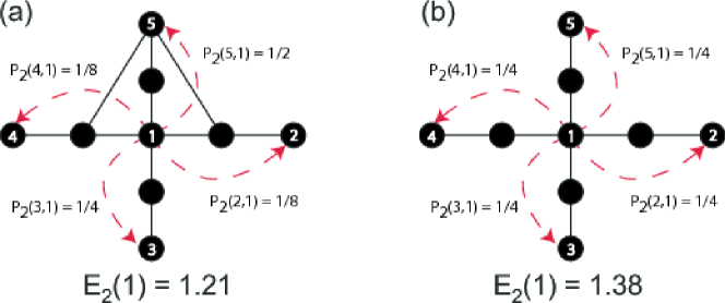
Figure 1: Illustration of the concept of diversity entropy: (a) node $1$ has low diversity entropy ($E_{2}(1)=1.21$) as a consequence of its unbalanced transition probabilities to the nodes reachable after two steps of a self-avoiding random walk; and (b) node $1$ has the highest diversity ($E_{2}(1)=1.38$) considering four accessible nodes.

Though the relationship between diversity entropy and the internality of the nodes had been hinted previously [7, 8], the present work reports a systematic investigation of such a definition of the borders of networks from several perspectives while taking into account model (theoretical) and real-world networks. After formally defining the concept of internality of each individual node in any network, we provide some analytical motivation with respect to diffusion (i.e. random walks) in regular lattices. Then we focus on geographical networks, whose borders can be intuitively related to their geographical structure (everybody has a conceptual idea of the borders of a city, for example). It is shown that the geographical borders tend to be in close agreement with the topological borders identified by the diversity entropy for both 2D and 3D geographical structures. Then, we investigate how the concept of internality extends to non-geographical networks with respect to knitted networks [9], which are regular but non-geographical stochastic structures. We perform this study by making ‘holes’ in the original networks, so that the borders of the holes can be well-defined topologically as corresponding to the limits of the holes. We show that the diversity entropy approach can precisely identify the original borders created by the holes. Subsequently, we take into account rewired (by using the procedure described by Maslov and Sneppen in [10]) versions of geographical networks, which allows us a series of insights on how the borders of initially geographically-constrained networks change with perturbations. The important issue of quantifying the degree of possible correlations between the diversity entropy and well-established measurements such as the degree and betweenness centrality are also investigated. The results corroborate little interrelationship between diversity entropy and such measurements, implying that the former feature is indeed providing additional information about the structure of the network. We conclude the current work by analyzing real-world networks, namely the plant of the town of São Carlos (SP, Brazil) as well as the network of word associations in Lewis Carroll’s Alice’s Adventures in Wonderland. Remarkable results are obtained regarding both cases, including the identification of modules of internality in the town and centrality of words in Alice’s Adventures in Wonderland.

2 Materials and Methods

2.1 Basic Concepts

Complex Networks An unweighted and undirected complex network is a set of $N$ nodes linked by $E$ edges [3, 5] that can be described by the adjacency matrix $A_{i,j}$. This matrix has binary elements $a_{i,j}$ that represent the presence or absence of connection between each pair of nodes. When $a_{i,j}=1$ there is an edge between the node $i$ and the node $j$. Otherwise, $a_{i,j}=0$ indicates that there is no connection between them. The degree of the node $i$, $k_{i}$, is the number of nodes directly connected to $i$. This quantity is related with the adjacency matrix by the relation $k_{i}=\sum_{j=1}^{N}a_{i,j}$.

A walk of length $h$ over the network is defined by a subset of $h+1$ adjacent nodes (i.e., nodes that share at least one edge). Considering a discrete time Markovian process over the network, the transition probability $P_{h}(j,i)$ is the probability that an agent departing from node $i$ reaches the node $j$ after $h$ steps. This probability can vary accordingly to the type of walk that is adopted. In the case of self-avoiding random walks, the moving agent cannot repeat nodes or edges during the walk [7, 8], while in traditional random walks the agent has no restriction to perform the walk [11]. We used self-avoiding random walks for all the examples presented in this paper, as with this dynamics it is possible to reach more nodes in fewer steps.

Diversity Entropy The diversity entropy of a particular node $i$ measures how diverse is the access from this node to the other nodes of the network through a walk of length $h$. Let $\Omega$ be the set of all nodes of the network, except $i$, and $N$ be the number of nodes of the network. The normalized diversity entropy $E_{h}(\Omega,i)$ can be expressed as [7, 8]

$$E_{h}(\Omega,i)=-\frac{1}{log(N-1)}\sum_{j=1}^{N}\left\{\begin{array}[]{rll}P_{h}(j,i)log(P_{h}(j,i))&\textrm{if $P_{h}(j,i)\neq 0$}\\ 0&\textrm{if $P_{h}(j,i)=0$}\\ \end{array}\right.$$ (1)

2.2 Border Detection

The concept of diversity is intuitively related to the definition of the border of a network. The main idea behind this property is that the peripheral nodes have not many options for proceeding a random walk other than accessing the internal nodes of the network, resulting in low diversity values [8]. On the other hand, non-border nodes tend to have more effective and balanced access to the most part of the internal and peripheral nodes of the network, resulting in high diversity entropy values. In order to demonstrate this property analytically, we resourced to a bidimensional grid, as explained below.

2.2.1 A theoretical approach

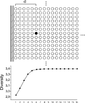
Figure 2: Illustration of the border effects on diversity entropy. (a) A semi-infinite grid network with border. The central node is painted in black and $d$ is the distance between the central node and the border. (b) Diversity entropy as function of the distance $d$ from the border.

Let us consider a bidimensional semi-infinite grid illustrated in figure 2. We want to investigate the diversity entropy of the central node (shown in black in figure 2) located at distance $d$ from the border of the grid. We start by evaluating the number of random walks of length $h$ between the central node and the node at the coordinate $(x,y)$, which is given by:

$$W_{h}(x,y)={\cal C}(h,x){\cal C}(h,y)-\beta_{h}(x,y)$$ (2)

where ${\cal C}$ denotes the binomial symbol and

$$\beta_{h}(x,y)=\left\{\begin{array}[]{l}{\cal C}(h,d+x+1){\cal C}(h,d+y+1)\\ \;\;\;\;\;\quad\mbox{if $x,y\leq h-d-1$ and $x+y\geq h-d-1$}\\ 0\\ \;\;\;\;\;\quad\mbox{if $x,y\leq h-d-1$ and $x+y<h-d-1$}\end{array}\right.$$

The probability that a walker reaches the node at coordinate $(x,y)$ after $h$ steps starting at the central node is

$$P_{h}(x,y)=\frac{W_{h}(x,y)}{\sum_{m}\sum_{n}W_{h}(m,n)}$$ (3)

Then, the diversity entropy of the central node is

$$E_{h}=-\frac{1}{\log(N-1)}\sum_{x}\sum_{y}P_{h}(x,y)\log\left(P_{h}(x,y)\right)$$ (4)

Observe that the sums run over all coordinates for which the value of $P_{h}(x,y)$ is not null. Figure 2(b) shows the diversity entropy as function of the distance $d$ of the central node from the border, considered a fixed walk length step of $h=7$. Note that in this figure the value of diversity entropy is lower near the border and constant when $d>h$ (i.e. the central node does not suffer border effects).

2.3 Border Detection Using Other Measurements

In addition to the diversity entropy, we also evaluate the use of other measurements in order to define de border of networks. The considered features include: the node degree, the average shortest path length (ASPL), and betweenness centrality ($B$). The ASPL for the node $i$ is the average length of all shortest path between $i$ and all other nodes of the network [5]. The betweenness centrality of the node $i$ is defined as $B_{i}=\sum_{i\neq p\neq q}\sigma_{p,q}(i)/\sigma_{p,q}$, where $\sigma_{p,q}$ is the number of shortest paths from $p$ to $q$ and $\sigma_{p,q}(i)$ is the number of shortest path from $p$ to $q$ that go through $i$ [5].

2.4 Datasets

In order to evaluate the efficiency of the proposed methodology, we used three hypothetical geographical networks with different shapes and physical constraints, such as bottlenecks and internal holes. Geographical networks were used as they are the only type of network where the border nodes can be defined visually, allowing immediate evaluation of the accuracy of the border-detection methodology.

Figure 3 shows the geographical networks adopted in our analysis. The first network, depicted in (a), consists of a single square-shaped network. The case (b) regards a network that includes bottlenecks (narrow connections) as well as internal holes. The third case, shown in (c), shows a sphere-shaped three-dimensional geographical network. In all cases, the nodes were generated by sampling spatial points in a space constrained by the bounding desired physical shape (e.g. points chosen within a circle of a given radius). The edges of the network were subsequently defined by Delaunay triangulation of the sampled points.

In order to validate the methodology for non-geographical networks, we performed the border detection over the Knitted model [9]. This network is built from a set of non connected nodes labeled from 1 to $N$. The basic step while growing this type of network involves shuffling the labels in an arbitrary sequence and defining the edges by connecting consecutive labels in that sequence. Note that the last label in the sequence is connected to the first one. This step is repeated $n$ times. As result of this process, we obtain a non-geographical network where all nodes have degree $k=2n$.

In addition to the hypothetical networks described above, we also considered two real-world examples of networks: the first refers to the network of urban streets of the Brazilian town of São Carlos. In this network, each node represents a street crossing or beginning of routes, while the edges represent the streets (see [8] for additional information); the second is a word association network, built considering the relationship between words in the Lewis Carroll book Alice’s Adventures in Wonderland. The nodes of this network represent the words, while the edges link the words that are adjacent in the text [12].

3 Results

This section presents six different results of the border detection methodology considering different measurements and data. First, the border of the geographical networks presented in figure 3 was detected in terms of the diversity entropy and self-avoiding random walks dynamics. Next, the results of the proposed methodology applied to non-geographical network are presented. In another analysis, we considered the border detection of a network four times denser than one of the networks of the first analysis. The next case shows an example of a geographical network that was progressively rewired and, again, the diversity entropy was used for border detection. Subsequently, the results of border detection using other measurements (node degree, betweenness centrality, and average shortest path length) are shown and discussed. Finally, the results of border detection with respect to the two real-world networks are presented and interpreted.

3.1 Detected borders using diversity entropy

The diversity entropy for the networks previously introduced were calculated considering five steps ($h=1..5$). The nodes of the networks shown in figure 3(a-c) were colored accordingly to their respective diversity entropy value for $h=3$. The classification of a node as border or non-border can be performed by choosing a threshold of the diversity at specific step. The nodes whose diversity entropy is below the threshold value are classified as border nodes. Figure 3(d-f) shows the detected border nodes (green nodes). Notably, in all analyzed networks the border nodes were successfully identified.

In addition, it is important to note that the thresholds used to obtain these results were automatically chosen. The following procedure was adopted: first, the minimum distance from each node to the contour of the shape (the physical border) was determined. The nodes nearest the border (i.e., have low distance values) were classified as border, while the others were understood as non-border nodes. Next, this classification was compared with the classification obtained by performing many consecutive thresholds of the diversity entropy value. The threshold value which result in the best relation between correctly classified border/non-border nodes was then used to define the border.

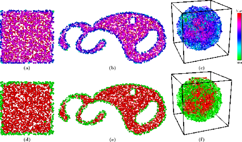
Figure 3: Border detection using diversity entropy with self-avoiding walks. (a-c) Three geographical networks used to evaluate the methodology. Each node is colored with respect to their diversity entropy value considering self-avoiding random walks and $h=3$. Note that the network in (c) is three-dimensional.(d-f) Results of the detection of the border (green nodes) by thresholding the diversity entropy.

3.2 Extension for non-geographical networks

In this section we give some insights about the extensibility of the diversity to detect borders in non-geographical networks. Unlike the case for geographical networks, the definition of border of non-geographical networks is not intuitive nor can be visualized. In order to address such networks, we development a methodology to assess the accuracy of the border detection methodology which basically consists in creating holes in a network. The main idea is to select a few nodes of the network and remove these nodes and their neighbors up to some pre-defined distance. By doing so, some holes in the network are created, and, as consequence, the neighbors of the removed nodes can be considered as border nodes. Then, after the identification of these border nodes, it is possible to evaluate the proposed border detection methodology by thresholding the diversity entropy and comparing the detected border with the actual borders defined by the holes.

This process is illustrated in figure 4. A knitted network with $N=300$ and $E=600$ is shown in figure 4(a). The hole in this network was obtained by removing the node with the highest diversity entropy value (note that other criteria could also be used) and its neighbors up to distance two. The border defined by this process is shown in figure 4(b) (green nodes), while the borders defined by thresholding the diversity entropy is shown in figure 4(c). Note that the results are quite good, with only a few misdetected nodes (4 nodes). For this analysis, the threshold was automatically chosen in a procedure very similar to that used in the geographical networks, with the difference that instead of using the distance from the physical border to define the actual border nodes, the nodes next to the hole were defined as the actual border.

In addition to the analysis of the border detection on a knitted network, we also tried the same procedure on a Barabási-Albert network (BA) [3]. However, the obtained results for a series of experiments showed that the ratio between correctly detected border/non-border were not satisfactory. The main reason for this result is that the average shortest path length in these networks is usually very low (e.g., this value is only 7 in a network with $N=1,000,000$ and $<k>=4$). As a consequence, the vast majority of the nodes of the network will be very close to the border defined by the holes, and their diversity entropy will be reduced (due to the proximity to the border). This reduction increases substantially the chances of misclassification. It is important to stress that the hole approach being unsuitable to evaluate the border detection methodology on BA networks does not invalidate our methodology. Given the other results reported in this work, as well as the own motivation for defining the borders as nodes of low diversity, it is reasonable to expect that the method will also correctly identify the borders in small-world networks such as Barabási-Albert.

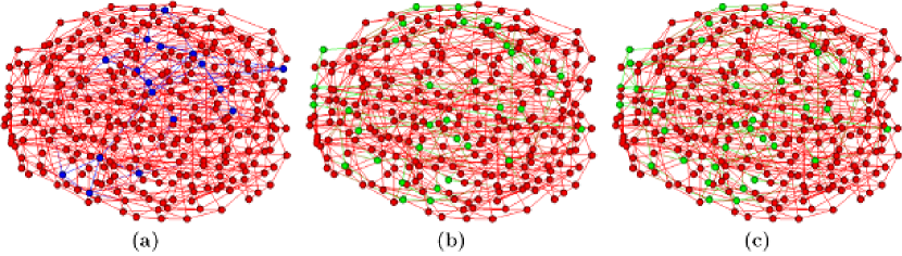
Figure 4: Border detection on a knitted network. (a) Original network where the blue nodes are removed in order to insert a hole on the network. (b) Network with a hole. The green nodes represent the border of this network. (c) Border detection using diversity entropy (green nodes represent the border nodes). Note that the obtained border is quite similar to the actual borders shown in (b).

3.3 Border detection for a denser network

This section reports a comparison of the results of the proposed border detection methodology considering networks with the same shape but with different density of nodes. For this purpose, we resourced to networks that contain narrow regions and holes (figure 3b), as well as a version of the same networks four times denser (with reference to nodes per square unit), shown in figure 5a. For the latter case, the border detection methodology was applied, i.e., the diversity entropy considering self-avoiding walks was calculated and a threshold on the diversity value was used to define the border (green nodes in figure 5).

The main difference between the results obtained for the two considered networks refer to the narrow regions of the shapes. The zoomed squares in figure 5 show some of these regions for both networks. While most of the nodes situated in narrow regions in the less dense network are considered as border, in the denser network only the most peripheral nodes of these regions are classified as borders. This result shows that the method is sensible to the spatial resolution of the nodes of the geographical network.

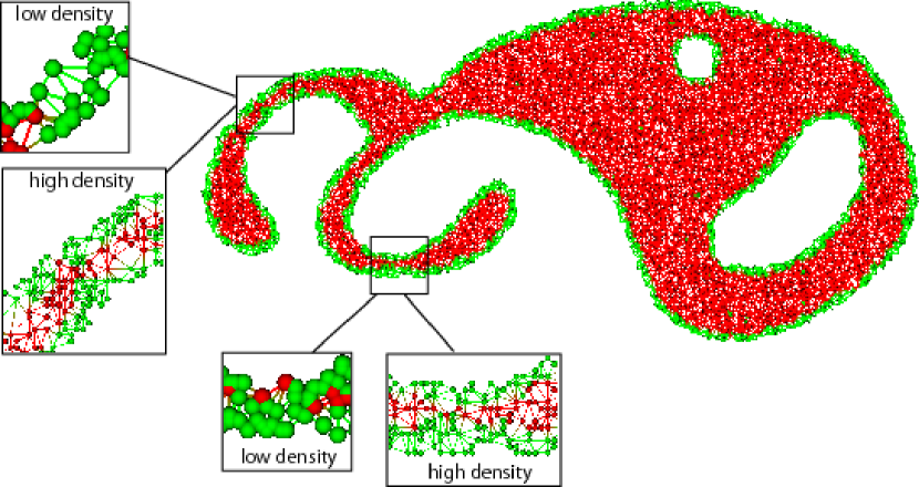
Figure 5: Border detection for a denser network. This network has the same shape of the network shown in figure 3b, but it is four times denser. The border nodes were detected (green nodes) and, when compared with the results obtained for the less dense network (figure 3f), it can be seen that the obtained results are quite similar. Note that, as shown by the zoomed regions, the main differences between these two networks can be found in the narrow regions, associated to smaller spatial and topological scales.

3.4 Border detection in a rewired network

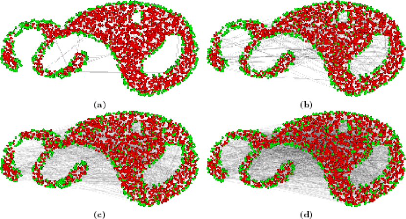
Figure 6: Border detection in a rewired network. The network shown in figure 3b had 0.1% (a), 1% (b), 5% (c) and 10% (d) of its edges rewired and the border was detected (green nodes). (a) Due to the low percentage of rewiring, no significant changes were detected during border detection. (b-d) When considering higher percentage of rewiring, a dislocation of the border to the internal regions of the networks can be clearly identified.

In this section we address the results of the border detection methodology when applied to rewired versions of geographical networks. Note that, when using rewired versions of a network it is reasonable to consider that part of the properties of the original (non-rewired) network are maintained, i.e., some regions of the rewired networks will still have the properties implied by the physical constraints while others will acquire non-geographical behavior (e.g. emergence of small world effect). Therefore, it is expected that the border detection methodology applied to these rewired network will not consider as border some of the former border nodes and additionally it will classify as border some of the former internal (non-border) nodes.

In order to evaluate this process, four different rewired versions of the network presented in figure 3b were analyzed. Figure 6 shows the obtained networks with 0.1% (a), 1% (b), 5% (c) and 10% (d) of rewired edges. Note that, in this figure, the nodes are already colored accordingly to the border/non-border classification. The threshold criteria used to define the border in all cases was the same used previously, i.e., the configuration which best approximates the physical border of the original network. That is the reason why many of the detected border nodes still remain near of the physical border. Particularly, for the first case, (a), the very low percentage of rewiring did not change the properties of the network and, as a consequence, the obtained result is quite similar to the original, non-rewired network. On the other hand, for the three remainder cases, the classification of the nodes as border nodes included some former internal nodes and excluded some former border nodes. Note that this result can also be understood as an extension of the proposed methodology to non-geographical networks.

3.5 Detected borders using node degree, betweenness centrality and average shortest path length

The results of the border detection obtained by using the node degree, the betweenness centrality and the average shortest path length are shown in the figures 7, 8, and 9. For all cases, the best threshold value was chosen in the same way described previously. Among these three measurements, the best result was found for the node degree. In this case, the border was properly detected at the expense that many internal nodes, which are not border, were classified as border. The same issue occurs, in a worse manner, when the betweenness centrality is used to detect the borders. Finally, when using the ASPL to detect the borders, it is clear from figure 9(a-b) that only the nodes located far from the geographical center of the network are classified as border, resulting in a completely incorrect result. In figure 9(c), the detection of the border presented a similar result with respect to the result obtained by using the diversity entropy.

In order to investigate the relationship between these three measurements and the diversity entropy, Table 1 shows their Pearson correlation coefficients. It can be noted from this table that no significant correlation was found with respect to any of the three considered networks, except for the network from figure3(c) (3D sphere), whose diversity entropy presented high correlation with the ASPL.

Network	DV x Degree	DV x BC	DV x ASPL
Figure 3(a)	0.73	0.56	-0.59
Figure 3(b)	0.76	0.18	-0.42
Figure 3(c)	0.76	0.72	-0.91

Table 1: Pearson correlation coefficients. DV: Diversity entropy; ASPL: Average shortest path length; BC: Betweenness centrality.

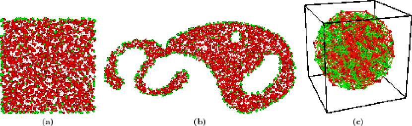
Figure 7: Border detection using the node degree. Although the border was properly detected, many internal nodes were also considered as border.

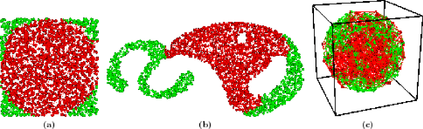
Figure 8: Border detection using the average shortest path length. In contrast with the diversity entropy, many nodes were misclassified.

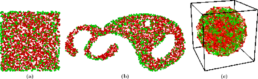
Figure 9: Border detection using the betweenness centrality. In this case, the noise level is high, i.e. the amount of internal nodes classified as border is high. This is a consequence of the fact that the betweenness centrality can assume low values even for the nodes located in the internal region of the network.

3.6 Real-world examples

In order to best illustrate the potential of the proposed methodology, in this section we present the results considering two real-world network examples: the geographical network of the urban streets of São Carlos and the word association network derived from the book Alice’s Adventures in Wonderland.

The network of the streets of São Carlos has $N=4537$ nodes and $E=7527$ edges. The diversity entropy was estimated for $h=1..5$. In order to determine the borders of this network, the threshold of the diversity entropy was manually chosen. The obtained result is shown in figure 10, where the green nodes represent the border nodes. This figure also shows the railway and the highways that cross the urban perimeter of the city. These structures impose important physical constraints in the planning of the streets of the city, slicing the urban area and giving rise to many border nodes along these ways. Observe that such border nodes, though not being directly related to the periphery of the network, were all properly detected by the proposed diversity methodology.

The second real-world example analyzed, the word association network from the book Alice’s Adventures in Wonderland, has $N=1929$ nodes and $E=9290$ edges. This network was built considering the words as nodes and by linking adjacent words in order to define the edges. To reduce the size of the network, the words were lemmatized (i.e. reduced to their canonical form) and the stop-words (e.g. the verb to be, prepositions, conjunctions, pronouns and articles) were not considered. In addition, we excluded the nodes of the network which had less than two connections and selected the biggest connected component of the remainder network. The resulting network, which has $N=505$ and $E=1102$, is shown in figure 11. The diversity entropy was computed for this network ($h=1..5$) and the ten lowest and highest values, together with their corresponding word, are shown in figure 11. It is clear that the most internal words (corresponding to the most internal nodes) seem to correspond to the most important terms in the book, while the border words tend to present a secondary nature regarding the main subjects in this book. In this sense, it is possible that the diversity quantifies in some way the centrality of words and concepts in texts.

Figure 12 shows the Pearson correlation coefficients obtained for the above two real networks considering the diversity entropy and the other three previously introduced measurements: degree, betweenness centrality, and ASPL. The obtained results indicate that there is no strong correlation between these measurements.

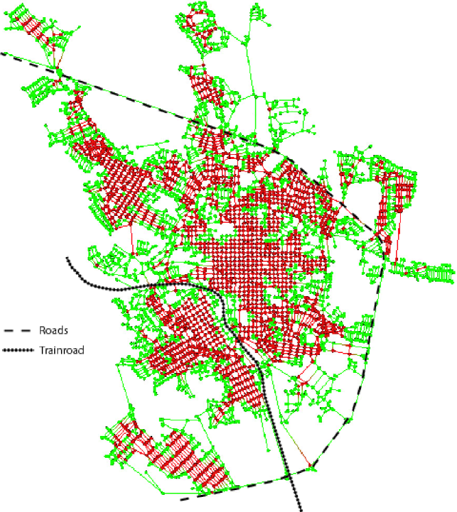
Figure 10: Border detection in the network of urban streets of the town of São Carlos - SP - Brazil. The border is indicated by the green nodes. Note that the highway and railroad that cross this town also defined specific borders which were properly identified by the diversity methodology.

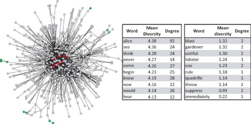
Figure 11: Network derived from words relationship in the book Alice’s Adventures in Wonderland. The green and red nodes represent the lowest and highest values of diversity entropy, respectively. The words corresponding to these nodes, as well their diversity entropy and degree, are shown in the side tables. Interesting, the node with highest degree (130), which correspond to the verb say, does not appear in the above list.

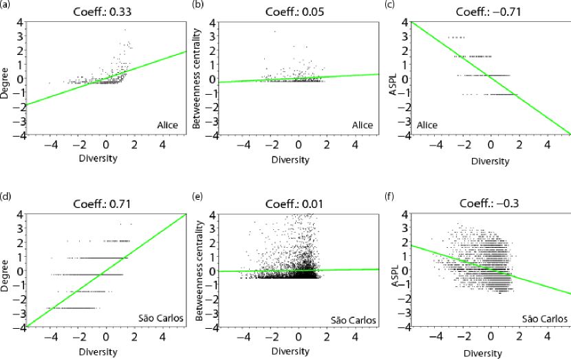
Figure 12: Pearson correlation coefficients between the diversity entropy and the number of neighbors (a,d), the between centrality (b,e) and ASPL (c,f) considering the word association network (a-c) and the streets network (d-f). Note that no considerable correlation between these measurements was identified for these networks (Coeff.: Pearson correlation coefficient).

4 Conclusions

Despite all the current investigations in complex networks research, some important related issues have received little attention. Given that real-world networks are necessarily finite, one important aspect concerns the definition and identification of their borders, a concept immediately related to internality/externality of nodes. The current work has addressed these important problems. More specifically, we used the recently introduced concept of diversity (e.g. [7, 8]) in order to quantify the potential of accessibility from and to each node while considering a specific dynamics, in the present case self-avoiding random walks. Nodes with more balanced transition probabilities to other nodes, expressed in terms of entropy, are understood as being more internal to the network, while the other nodes are associated to the network borders.

The concept of borders is immediate and intuitive in geographical networks, where the more internal nodes are usually found at the geometrically more internal regions. Therefore, we give special attention to this type of networks in order to motivate and validate our approach. Interestingly, the application of the diversity methodology to geographical networks identified as borders not only the nodes at the peripheral regions, but also those nodes which are geographically more internal but are near geographical discontinuities slicing the network. The definition of borders in non-geographical networks has been an important open question. We showed that it is possible to extend the diversity approach to define and identify borders in that type of networks. We also compared the diversity approach with methods founded on other measurements such as degree, betweenness centrality and average shortest path lengths. None of these alternative approaches turned out not to be able to properly detect the borders, even in the case of geographical networks. We also found no significant correlation between the diversity and those measurements, which further corroborates that that feature does provide additional information about the topology of the networks. The potential of the methodology proposed for the identification of the borders was illustrated with respect to both theoretical (i.e. regular, geographical and knitted networks) and real-world networks (i.e. the urban network of the town of São Carlos and Carroll’s Alice’s Adventures in Wonderland). Several findings and insights were yielded by the adopted approach, including the impressive performance for identification of the borders in knitted networks, a non-geographical structure. In addition, it was showed that the urban network presents borders not only at its periphery, but also along the railway line and highway that happen to cross that town. In the case of Carroll’s work, the most internal words tended to be more immediately related to the main thematic of the book, while the most external nodes (borders) related to secondary concepts.

The effectiveness of the reported approach has paved the way to a number of promising further investigations, including its application for the identification of the borders in several important real-world networks such as gene regulation, airports, and anatomical networks [13]). A particularly interesting prospect would be to apply the methodology to detect the borders in pictures where the objects do not have well-defined contours (e.g. are composed by textures and clouds).

References

References

- [1] A. Barabási and R. Albert. Emergence of scaling in random networks. Science, 286:509, 1999.
- [2] Michalis Faloutsos, Petros Faloutsos, and Christos Faloutsos. On power-law relationships of the internet topology. In SIGCOMM ’99: Proceedings of the conference on Applications, technologies, architectures, and protocols for computer communication, pages 251–262, New York, NY, USA, 1999. ACM.
- [3] Albert and A.-L. Barabási. Statistical mechanics of complex networks. Rev. Mod. Phys., 74:47, 2002.
- [4] S. Boccaletti, V. Latora, Y. Moreno, M. Chavez, and D. U. Hwang. Complex networks : Structure and dynamics. Physics Reports, 424(4-5):175–308, 2006.
- [5] L. da F. Costa, F. A. Rodrigues, G. Travieso, and P. R. Villas Boas. Characterization of complex networks: A survey of measurements. Advances In Physics, 56:167, 2007.
- [6] L. da F. Costa, O. N. Oliveira Jr., G. Travieso, F. A. Rodrigues, P. R. Villas Boas, L. Antiqueira, M. P. Viana, and L. E. C. da Rocha. Analyzing and modeling real-world phenomena with complex networks: A survey of applications. arXiv:0711.3199, 2007.
- [7] L. da F. Costa. Inward and outward node accessibility in complex networks as revealed by non-linear dynamics. Preprint cond-mat/0801.1982, 2008.
- [8] B. A. N. Travencolo and L. F. Costa. Hierarchical spatial organization of geographical networks. Journal of Physics A: Mathematical and Theoretical, 41(22):224004+, 2008.
- [9] L. da F. Costa. Knitted complex networks. Preprint arXiv:0711.2736v1, 2007.
- [10] S. Maslov and K. Sneppen. Specificity and stability in topology of protein networks. Science, 296(5569):910–913, 2002.
- [11] J. D. Noh and H. Rieger. Random walks on complex networks. Physical Review Letters, 92:118701, 2004.
- [12] L. Antiqueira, T. A. S. Pardo, M. G. V. Nunes, and O. N. Oliveira Jr. Some issues on complex networks for author characterization. Revista Iberoamericana de Inteligencia Artificial, 11(36):51–58, 2007.
- [13] Matheus P. Viana, Bruno A. N. Travencolo, E. Tanck, and Luciano da F. Costa. Characterizing the diversity of dynamics in complex networks without border effects. Preprint cond-mat/0805.2298, 2008.