Detecting a conditional extreme value model

Abstract.

In classical extreme value theory probabilities of extreme events are estimated assuming all the components of a random vector to be in a domain of attraction of an extreme value distribution. In contrast, the conditional extreme value model assumes a domain of attraction condition on a sub-collection of the components of a multivariate random vector. This model has been studied in Heffernan and Tawn (2004), Heffernan and Resnick (2007), Das and Resnick (2008b). In this paper we propose three statistics which act as tools to detect this model in a bivariate set-up. In addition, the proposed statistics also help to distinguish between two forms of the limit measure that is obtained in the model.

1. Introduction

Extreme value theory (henceforth abbreviated EVT) is used to model environmental, financial and internet traffic data. Multivariate extreme value theory assumes an extreme-valued domain of attraction condition on the joint distribution of a random vector which after a suitable standardization relates multivariate extreme value theory to regular variation on $\mathbb{R}_{+}^{d}$. Probabilities of critical risk events can be estimated under the regularly varying assumption and then related back to the original co-ordinate system. Such estimates are a function of the dependence structure among the variables in the multivariate model. There is a substantial literature on the behavior of multivariate extreme-value theory both in the presence of asymptotic dependence and asymptotic independence (Coles and Tawn, 1991, Ledford and Tawn, 1996, 1997, 1998, de Haan and de Ronde, 1998, Resnick, 2002, Maulik and Resnick, 2005, de Haan and Ferreira, 2006).

A conditional extreme value (CEV) model was proposed in Heffernan and Tawn (2004), where multivariate distributions were approximated by conditioning on one of the components being in an extreme-value domain. The authors showed that this approach incorporated a variety of examples of different types of asymptotic dependence and asymptotic independence. Their statistical ideas were given a more mathematical framework by Heffernan and Resnick (2007) after slight changes in assumptions to make the theory more probabilistically viable. A further study (Das and Resnick (2008b)) revealed that assuming a conditional extreme value model holds no matter what conditioning variable is chosen is equivalent to assuming a multivariate extreme-value domain of attraction on the entire random vector. It is known that in the presence of asymptotic independence, the limit measure in the multivariate EVT set up has an empty interior; in other words, the limit measure concentrates on the boundary of the state space. In such a case an additional assumption of a CEV model provides more insight into the dependence structure. The CEV model also provides a way for modeling multivariate data assuming a subset rather than the entire vector to be extreme-valued. In this paper we suggest situations where a CEV model can be used and suggest techniques to detect the model and in the process also detect characteristics of the limit measure for the model. The methodologies are suggested for a bivariate data set.

Section 1 provides an introduction and review of the model. Section 2 deals with the detection of a conditional extreme value model. It has been shown in Das and Resnick (2008b) that the CEV model can be standardized to regular variation on a special cone if and only if the limit measure involved is not a product. In case of a product measure in the limit, we need to estimate fewer parameters and calculating probabilities is also simpler. Fougères and Soulier (2008) suggests some estimates for parameters and normalizing constants in the two different cases (product and non-product limit measures). Hence it is important to know whether we are in the product case or not. In Section 2 we propose three statistics whose behavior can first of all indicate the appropriateness of the CEV model and secondly indicate whether the limit measure is a product or not. Section 3 is dedicated to applying our techniques to some simulated and real data coming from Internet traffic studies.

1.1. Preliminaries: The CEV model and some related results

We discuss the model and preliminary results in this subsection. Refer to Heffernan and Resnick (2007) and Das and Resnick (2008b) for further discussion on conditional extreme value models.

A univariate extreme value distribution $G_{\gamma}$, for $\gamma\in\mathbb{R}$, is defined as

(1.1) $$G_{\gamma}(x)=\exp\{-(1+\gamma x)^{-1/\gamma}\},\qquad x\in\mathbb{E}^{(\gamma)},$$

where $\mathbb{E}^{(\gamma)}=\{x\in\mathbb{R}:1+\gamma x>0\}$. For $\gamma=0$, the distribution function is interpreted as $G_{0}(x)=e^{-e^{-y}},\,y\in\mathbb{E}^{(0)}:=\mathbb{R}$. We let $\overline{\mathbb{E}}^{(\gamma)}$ be the right closure of $\mathbb{E}^{(\gamma)}$; that is,

$$\overline{\mathbb{E}}^{(\gamma)}=\begin{cases}(-\frac{1}{\gamma},\infty]&\gamma>0,\\ (-\infty,\infty]&\gamma=0,\\ (-\infty,-\frac{1}{\gamma}]&\gamma<0.\end{cases}$$

Let $(X,Y)$ be a random vector in $\mathbb{R}^{2}$. For a CEV model we make the following assumptions:

1. The distribution $F(x):=P[Y\leq x]$ is in the domain of attraction of an extreme value distribution, $G_{\gamma}$, written $F\in D(G_{\gamma})$. This means there exist functions $a(t)>0$, $b(t)\in\mathbb{R}$ such that, as $t\to\infty$,

   (1.2) $$t(1-F(a(t)y+b(t)))=t\mathbf{P}\biggl{(}\frac{Y-b(t)}{a(t)}>y\biggr{)}\to(1+\gamma y)^{-1/\gamma},\qquad 1+\gamma y>0,$$

   for $y\in\mathbb{E}^{(\gamma)}.$

2. There exist functions $\alpha(t)>0$ and $\beta(t)\in\mathbb{R}$ and a non-null Radon measure $\mu$ on Borel subsets of $[-\infty,\infty]\times\overline{\mathbb{E}}^{(\gamma)}$ such that for each $y\in\mathbb{E}^{(\gamma)}$,

   (1.3) $$[a]\quad t\mathbf{P}\biggl{(}\frac{X-\beta(t)}{\alpha(t)}\leq x,\frac{Y-b(t)}{a(t)}>y\biggr{)}\to\mu([-\infty,x]\times(y,\infty]),\quad\text{ as }t\to\infty,$$

         for $$(x,y)$$ continuity points of the limit,

   (1.4) $$[b]\quad\mu([-\infty,x]\times(y,\infty])\quad\text{ is not a degenerate distribution in $x$},$$

   (1.5) $$[c]\quad\mu([-\infty,x]\times(y,\infty])<\infty.$$

   (1.6) $$[d]\quad H(x):=\mu([-\infty,x]\times(0,\infty])\text{ is a probability distribution.}$$

A non-null Radon measure $\mu(\cdot)$ is said to satisfy the conditional non-degeneracy conditions if both of (1.4) and (1.5) hold. We say that $(X,Y)$ follows a conditional extreme value model (or CEV model) if conditions (1) and (2) above are satisfied. The reason for this name is that, assuming $(x,0)$ to be a continuity point of $\mu$, (1.3), (1.4) and (1.5) imply that

(1.7) $$\mathbf{P}\biggl{(}\frac{X-\beta(t)}{\alpha(t)}\leq x\bigg{|}Y>b(t)\biggr{)}\to H(x)=\mu([-\infty,x]\times(0,\infty])\qquad(t\to\infty).$$

Note that (1.3) can be viewed in terms of vague convergence of measures in $\mathbb{M}_{+}\bigl{(}[-\infty,\infty]\times\overline{\mathbb{E}}^{(\gamma)}\bigr{)}$, the space of Radon measures on $[-\infty,\infty]\times\overline{\mathbb{E}}^{(\gamma)}$.

In this model the transformation $Y\mapsto Y^{*}=b^{\leftarrow}(Y)$ standardizes the $Y$-variable, i.e., we can assume $a^{*}(t)=t,b^{*}(t)=0$. Hence a reformulation of (1.3) leads to

(1.8) $$t\mathbf{P}\biggl{(}\frac{X-\beta(t)}{\alpha(t)}\leq x,\frac{Y^{*}}{t}>y\biggr{)} \to\mu^{*}([-\infty,x]\times(y,\infty]),\quad\text{ as }t\to\infty,$$

for $$(x,y) \mu^{*}$$ continuity points of where,

(1.9) $$\mu^{*}([-\infty,x]\times(y,\infty]) =\begin{cases}\mu\bigl{(}[-\infty,x]\times(\frac{y^{\gamma}-1}{\gamma},\infty]\bigr{)},&\text{ if }\gamma\neq 0,\\ \mu\bigl{(}[-\infty,x]\times(\log y,\infty]\bigr{)},&\text{ if }\gamma=0.\\ \end{cases}$$

We also know (Heffernan and Resnick, 2007, Proposition 1) that the following variational property holds: there exists functions $\psi_{1}(\cdot),\psi_{2}(\cdot)$ such that for all $c>0$,

(1.10) $$\lim\limits_{t\to\infty}\frac{\alpha(tc)}{\alpha(t)}=\psi_{1}(c), \lim\limits_{t\to\infty}\frac{\beta(tc)-\beta(t)}{\alpha(t)}=\psi_{2}(c).$$

This implies that $\psi_{1}(c)=c^{\rho}$ for some $\rho\in\mathbb{R}$ (de Haan and Ferreira, 2006, Theorem B.1.3). Also, $\psi_{2}$ can be either 0 or $\psi_{2}(c)=k\frac{c^{\rho}-1}{\rho}$ for some $k\neq 0$ (de Haan and Ferreira, 2006, Theorem B.2.1).

Remark 1.1.

The CEV model primarily differs from the multivariate extreme value model in the domain of attraction condition. Das and Resnick (2008b) provides conditions under which a CEV model can be extended to multivariate extreme value model. Under the multivariate extreme value model, each of the variables can be standardized so that we have a multivariate regular variation on the cone $[\boldsymbol{0},\boldsymbol{\infty}]\setminus\{\boldsymbol{0}\}$; see de Haan and Resnick (1977) and Chapter 6 of de Haan and Ferreira (2006). The conditional extreme value model can be standardized if and only if the limit measure $\mu$ in (1.3) is not a product measure (Das and Resnick, 2008b). When both $X$ and $Y$ are standardized, we can characterize the limit measure in terms of all Radon measures (finite and infinite) on $[0,1)$. Though theoretically elegant, performing standardization in practice is not an easy task.

Thus, it is important to know when the limit is a product measure. A product measure in the limit precludes standardization of both the variables (Heffernan and Resnick, 2007) and means that we do not have a multivariate extreme value model (Das and Resnick, 2008b). However, a product measure makes the estimation of certain parameters and probabilities easier. For instance, in the product case $(\psi_{1},\psi_{2})\equiv(1,0)$ so $\rho=0$ (see (1.10)) but without the property that $\mu$ is a product, $\rho$ has to be estimated. Furthermore, the limit being a product measure can be considered as a form of asymptotic independence in the CEV model, which can be probabilistically useful (Maulik et al., 2002).

1.2. Appropriateness of the CEV model.

Multivariate extreme value theory provides a rich literature on estimation of probabilities of extreme regions containing few or no data points in the sample. The multivariate theory assumes that each variable is marginally in an extreme value domain of attraction. However, this might not be the right assumption for all data sets. We encounter data where one or some but not all the variables can be assumed to be in an extreme value domain; see Section 3.2. The CEV model is a candidate model in such cases.

Another circumstance where the CEV model can be helpful is if one has a multivariate extreme value model with limit measure $\nu$ possessing asymptotic independence. This means that in the standardized model, the limit measure, $\nu^{*}(\cdot)$, concentrates on the axes through $\{\boldsymbol{0}\}$ and $\nu^{*}((\boldsymbol{0},\boldsymbol{\infty}])=0$. So an estimate of the probability of a region where both variables are big will turn out to be zero which may be a useless and misleading estimate. In such a circumstance, finer estimates can be obtained using either hidden regular variation (Maulik and Resnick, 2005) or the CEV model. Both methods provide a non-zero limit measure by using normalization functions which are of different order from the multivariate EV model. The relationship between the multivariate EV model and the CEV model and the respective normalizing functions considered in Das and Resnick (2008b).

So, how do we decide if the CEV model is appropriate for multivariate data?

1. Start by checking whether any of the marginal variables belongs to the domain of attraction of an extreme value distribution. An informal way to do this is through plots of the estimators of the extreme value parameter $\gamma$ (Pickands plot, Moment estimator plot, etc). If the plot attains stability in some range it is reasonable to assume an extreme-value model. More formal methods for testing membership in a domain of attraction using quantile and distribution functions are discussed in de Haan and Ferreira (2006), Chapter 5.2. The special case of a heavy-tailed random variable can be detected using the QQ plot, plotting the theoretical quantiles of the exponential distribution versus the logarithm of the sorted data and checking for linearity in the high values of the data. This is reviewed in Resnick (2007) and Das and Resnick (2008a).

2. If some, but not all, marginal variables are in a domain of attraction, proceed to see if the data is consistent with the CEV model. See Section 2.

3. If all variables are in some extreme value domain, check if the multivariate extreme value model is appropriate and if asymptotic independence is present. One way to do this is by checking whether both maximum and minimum of the standardized variables have distributions with regularly varying tails (Coles et al., 1999, Resnick, 2002). If the EV model is appropriate and asymptotic independence is absent, the CEV model does not provide any more information than the EV model. On the other hand if asymptotic independence is present, the CEV model, if detected, provides supplementary information about the joint behavior of the variables away from at least one of the axes.

2. Three estimators for detecting the CEV model

Let $(X_{1},Y_{1}),\ldots,(X_{n},Y_{n})$ be a bivariate random sample. In this section we propose three statistics to detect whether our sample is consistent with the CEV model under the assumption that at least one of the variables is in an extreme-value domain, and without loss of generality we assume $Y$ to be that variable. Our statistics have a consistency property which allows detection of a product form for the limit measure.

Assume $(X_{1},Y_{1}),\ldots,(X_{n},Y_{n})$ is iid from a CEV model as defined in Section 1.1. We first formulate a consequence of (1.3) which will be convenient for our purpose. The following notations will be used.

$$\begin{array}[]{llll}Y_{(1)}\geq\ldots\geq Y_{(n)}&\text{The decreasing order statistics of $Y_{1},\ldots,Y_{n}$.}\\[5.69054pt] X_{i}^{*},~{}1\leq i\leq n&\text{The $X$-variable corresponding to $Y_{(i)}$, also called the concomitant of $Y_{(i)}$.}\\[5.69054pt] R_{i}^{k}=\sum\limits_{l=i}^{k}\boldsymbol{1}_{\{X_{l}^{*}\leq X_{i}^{*}\}}&\text{Rank of $X_{i}^{*}$ among $X_{1}^{*},\ldots,X_{k}^{*}$. We write $R_{i}=R_{i}^{k}$.}\\[5.69054pt] X_{1:k}^{*}\leq X_{2:k}^{*}\leq\ldots\leq X_{k:k}^{*}&\text{The increasing order statistics of $X_{1}^{*},\ldots,X_{k}^{*}$.}\end{array}$$

2.1. A consequence for empirical measures

When the CEV property holds, a family of point processes of ranks of the sample converge vaguely to a Radon measure. By transforming to ranks of the data, we presumably lose efficiency since only the relative ordering in the sample remains unchanged but detection of the CEV property is easier since we no longer need to estimate the various parameters of the model. See de Haan and de Ronde (1998), de Haan and Ferreira (2006), Resnick (2007).

The convergence statement (1.3) of the CEV model defined in Section 1.1 can be interpreted in terms of vague convergence of measures. In preparation for the forthcoming result we recall some commonly used notation and concepts. Let $\mathbb{E}^{*}$ be a locally compact space with a countable base (for example, a finite dimensional Euclidean space). We denote by $\mathbb{M}_{+}(\mathbb{E}^{*})$, the non-negative Radon measures on Borel subsets of $\mathbb{E}^{*}$. If $\mu_{n}\in\mathbb{M}_{+}(\mathbb{E}^{*})$ for $n\geq 0$, then $\mu_{n}$ converge vaguely to $\mu_{0}$ (written $\mu_{n}\stackrel{{\scriptstyle v}}{{\to}}\mu_{0}$) if for all bounded continuous functions $f$ with compact support we have

$$\int_{\mathbb{E}^{*}}fd\mu_{n}\to\int_{\mathbb{E}^{*}}fd\mu_{0}\quad(n\to\infty).$$

This concept allows us to write (1.3) as

(2.1) $$t\mathbf{P}\Bigg{(}\Big{(}\frac{X-\beta(t)}{\alpha(t)},\frac{Y-b(t)}{a(t)}\Big{)}\in\cdot\Bigg{)} \stackrel{{\scriptstyle v}}{{\to}}\mu(\cdot),\quad\text{ as }t\to\infty$$

in $\mathbb{M}_{+}([-\infty,\infty]\times\overline{\mathbb{E}}^{(\gamma)})$. Standard references include Kallenberg (1983), Neveu (1977) and Resnick (2008, Chapter 3).

Recall the definition of $\mu^{*}$ in (1.9) and define the measure $L(\cdot)\in\mathbb{M}_{+}([0,1]\times[1,\infty])$ by

(2.2) $$L([0,x]\times(y,\infty])=\mu^{*}([-\infty,H^{\leftarrow}(x)]\times[y,\infty]),\quad(x,y)\in[0,1]\times(1,\infty].$$

Applying a reciprocal transformation to the second coordinate,

$$T_{0}:(x,y)\mapsto(x,y^{-1})$$

converts $L$ into the copula $L\circ T_{0}^{-1}$.

Proposition 2.1.

Suppose $(X_{1},Y_{1}),(X_{2},Y_{2}),\ldots,(X_{n},Y_{n})$ are i.i.d. observations from a CEV model which follows (1.2)-(1.6) and suppose $H$ is continuous. If $k=k(n)\to\infty,n\to\infty$ with $k/n\to 0$, then in $\mathbb{M}_{+}([0,1]\times[1,\infty])$

$$\frac{1}{k}\sum\limits_{i=1}^{k}\epsilon_{(\frac{R_{i}}{k},\frac{k+1}{i})}(\cdot)\Rightarrow L(\cdot).$$

Proof.

From (2.1) and (Resnick, 2007, Theorem 5.3(ii)), as $n,k\to\infty$ with $\frac{k}{n}\to 0$,

(2.3) $$\frac{1}{k}\sum\limits_{i=1}^{n}\epsilon_{\big{(}\frac{X_{i}-\beta(n/k)}{\alpha(n/k)},\frac{Y_{i}-b(n/k)}{a(n/k)}\big{)}}(\cdot) \Rightarrow\mu(\cdot),$$

in $\mathbb{M}_{+}([-\infty,\infty]\times\overline{\mathbb{E}}^{(\gamma)})$. Recall $Y_{(1)}\geq Y_{(2)}\geq\ldots\geq Y_{(n)}$ are the order statistics of $Y_{1},\ldots,Y_{n}$ in decreasing order and ordering the $Y$’s in (2.3) allows us to write the equivalent statement

(2.4) $$\frac{1}{k}\sum\limits_{i=1}^{n}\epsilon_{\big{(}\frac{X_{i}^{*}-\beta(n/k)}{\alpha(n/k)},\frac{Y_{(i)}-b(n/k)}{a(n/k)}\big{)}}\Rightarrow\mu(\cdot).$$

Define the measure $\nu_{\gamma}$ by

$$\nu_{\gamma}\bigl{(}(y,\infty]\cap\overline{\mathbb{E}}^{(\gamma)}\bigr{)}=(1+\gamma y)^{-1/\gamma},\quad y\in\mathbb{E}^{(\gamma)},$$

and sometimes, here and elsewhere, we sloppily write $\nu_{\gamma}(y,\infty]$. Taking marginal convergence in (2.3), or using (1.2), we have with that

$$\frac{1}{k}\sum\limits_{i=1}^{n}\epsilon_{\frac{Y_{i}-b(n/k)}{a(n/k)}}(\cdot) \Rightarrow\nu_{\gamma}(\cdot),$$

in $$\mathbb{M}_{+}(\overline{\mathbb{E}}^{(\gamma)}$$. Using an inversion technique (Resnick and Stărică (1995), de Haan and Ferreira (2006), Resnick (2007, page 82)), we get

(2.5) $$\frac{Y_{(\lceil(k+1)t\rceil)}-b(n/k)}{a(n/k)} \stackrel{{\scriptstyle\text{P}}}{{\to}}\frac{t^{-\gamma}-1}{\gamma},$$

in $D_{l}\bigl{(}(0,\infty],\overline{\mathbb{E}}^{(\gamma)}\bigr{)}$, the class of left continuous functions on $(0,\infty]$ with range $\overline{\mathbb{E}}^{(\gamma)}$ and with finite right limits on $(0,\infty)$. The convergence in (2.5) being to a non-random function, we can append it to the convergence in (2.4) to get the following (Billingsley, 1968, p.27):

$$(\mu_{n},x_{n}(t):= \Bigg{(}\frac{1}{k}\sum\limits_{i=1}^{n}\epsilon_{\big{(}\frac{X_{i}^{*}-\beta(n/k)}{\alpha(n/k)},\frac{Y_{(i)}-b(n/k)}{a(n/k)}\big{)}}(\cdot),\frac{Y_{(\lceil(k+1)t\rceil)}-b(n/k)}{a(n/k)}\Bigg{)}$$

(2.6) $$\Rightarrow \Big{(}\mu(\cdot),\frac{t^{-\gamma}-1}{\gamma}\Big{)}=(\mu,x_{\infty}(t))$$

on $\mathbb{M}_{+}([-\infty,\infty]\times\overline{\mathbb{E}}^{(\gamma)})\times D_{l}\bigl{(}(0,\infty],\overline{\mathbb{E}}^{(\gamma)})\bigr{)}$.

Let $D_{l}^{\downarrow}\bigl{(}(0,\infty],\overline{\mathbb{E}}^{(\gamma)})\bigr{)}$ be the subfamily of $D_{l}\bigl{(}(0,\infty],\overline{\mathbb{E}}^{(\gamma)})\bigr{)}$ consisting of non-increasing functions and define

$$T_{1}:\mathbb{M}_{+}([-\infty,\infty]\times\overline{\mathbb{E}}^{(\gamma)})\times D_{l}^{\downarrow}\bigl{(}(0,\infty],\overline{\mathbb{E}}^{(\gamma)})\bigr{)}\mapsto\mathbb{M}_{+}\bigl{(}[-\infty,\infty]\times(0,\infty]\bigr{)}$$

by

$$T_{1}(m,x(\cdot))=m^{*}$$

where

$$m^{*}([-\infty,x]\times(t,\infty])=m([-\infty,x]\times(x(t^{-1}),\infty]),\quad x\in[-\infty,\infty],\,t\in(0,\infty].$$

This is an a.s. continuous map so apply this to (2.6) and

(2.7) $$T_{1}(\mu_{n},x_{n})\Rightarrow T_{1}(\mu,x_{\infty}).$$

For $x\in[-\infty,\infty]$ and $y\in(0,\infty]$, the left side of (2.7) on the set $[-\infty,x]\times(y,\infty]$ is

$$\mu_{n}\bigl{(}[-\infty,x]\times(\frac{Y_{(\lceil(k+1)t\rceil)}-b(n/k)}{a(n/k)},\infty]\bigr{)}$$

and since

$$\frac{Y_{(i)}-b(n/k)}{a(n/k)}>\frac{Y_{(\lceil(k+1)t\rceil)}-b(n/k)}{a(n/k)}$$

iff

$$i<(k+1)y^{-1}\quad\text{ or }\quad\frac{k+1}{i}>y,$$

the left side of (2.7) on the set $[-\infty,x]\times(y,\infty]$ is

$$\frac{1}{k}\sum\limits_{i=1}^{n}\epsilon_{\big{(}\frac{X_{i}^{*}-\beta(n/k)}{\alpha(n/k)},\frac{k+1}{i}\big{)}}([-\infty,x]\times(y,\infty]).$$

The right side of (2.7) on the set $[-\infty,x]\times(y,\infty]$ is

$$\mu\bigl{(}[-\infty,x]\times(\frac{y^{\gamma}-1}{\gamma},\infty]\bigr{)}=\mu^{*}\bigl{(}[-\infty,x]\times(y,\infty]\bigr{)},$$

so we conclude

(2.8) $$\frac{1}{k}\sum\limits_{i=1}^{n}\epsilon_{\big{(}\frac{X_{i}^{*}-\beta(n/k)}{\alpha(n/k)},\frac{k+1}{i}\big{)}}\Rightarrow\mu^{*}$$

in $\mathbb{M}_{+}\bigl{(}[-\infty,\infty]\times(0,\infty]\bigr{)}.$ Recall $\mu^{*}(\cdot)$ was defined in (1.9).

Now assuming $(x,1)$ is a continuity point of $\mu^{*}$ we have

$$H_{n}(x):= \frac{1}{k}\sum\limits_{i=1}^{k}\epsilon_{\big{(}\frac{X_{i}^{*}-\beta(n/k)}{\alpha(n/k)},\frac{k+1}{i}\big{)}}([-\infty,x]\times(1,\infty])$$

(2.9) $$\Rightarrow \mu^{*}([-\infty,x]\times(1,\infty])=:H(x),$$

or in the topology of weak convergence on $PM[-\infty,\infty]$, the probability measures on $[-\infty,\infty]$,

$$H_{n}\Rightarrow H.$$

Define a map $T_{2}$ on $\mathbb{M}_{+}([-\infty,\infty]\times[1,\infty])\times PM[-\infty,\infty]$ by

$$T_{2}(m,G)=m^{\#}$$

where

$$m^{\#}([0,z]\times(y,\infty])=m([0,G(z)]\times(y,\infty])$$

or, for $f\in C([0,1]\times[1,\infty])$,

$$m^{\#}(f)=\iint f(G(x),y)m(dx,dy).$$

This map is continuous at $(m,G)$ provided $G$ is continuous. To see this, let $f$ be continuous on $[0,1]\times[1,\infty]$ and suppose $G_{n}\Rightarrow G$ and $m_{n}\stackrel{{\scriptstyle v}}{{\to}}m$. Then

$$\Bigl{|}\iint f(G_{n}(x),y) m_{n}(dx,dy)-\iint f(G(x),y)m_{n}(dx,dy)\Bigr{|}$$

$$\leq \Bigl{|}\iint f(G_{n}(x),y)m_{n}(dx,dy)-\iint f(G(x),y)m_{n}(dx,dy)\Bigr{|}$$

$$\qquad+\Bigl{|}\iint f(G(x),y)m_{n}(dx,dy)-\iint f(G(x),y)m(dx,dy)\Bigr{|}$$

$$= I+II.$$

For $I$, convergence to $0$ follows by uniform continuity of $f$ and the fact that $G_{n}(x)\to G(x)$ uniformly in $x$. To verify $II\to 0$, it suffices to note that $f(G(x),y)$ is continuous with compact support $[-\infty,\infty]\times[1,\infty]$ and then use $m_{n}\stackrel{{\scriptstyle v}}{{\to}}m$.

Combine (2.8) and (2.9) to get

(2.10) $$\Bigl{(}\frac{1}{k}\sum\limits_{i=1}^{k}\epsilon_{\big{(}\frac{X_{i}^{*}-\beta(n/k)}{\alpha(n/k)},\frac{k+1}{i}\big{)}},H_{n}\Bigr{)}\Rightarrow(\mu^{*},H)$$

in $\mathbb{M}_{+}\bigl{(}[-\infty,\infty]\times[1,\infty]\bigr{)}\times PM[-\infty,\infty]$. Apply the transformation $T_{2}$ discussed in the previous paragraph. The limit at $[0,x]\times(y,\infty]$ is $\mu^{*}\bigl{(}[-\infty,H^{\leftarrow}(x)]\times(y,\infty]\bigr{)}=L[0,x]\times(y,\infty]$. The converging sequence can be written as

$$\frac{1}{k}\sum_{i=1}^{k}\epsilon_{\Bigl{(}H_{n}\bigl{(}\frac{X_{i}^{*}-\beta(n/k)}{\alpha(n/k)}\bigr{)},\frac{k+1}{i}\Bigr{)}}.$$

Finally observe

$$H_{n}\bigl{(}\frac{X_{i}^{*}-\beta(n/k)}{\alpha(n/k)}\bigr{)}=\frac{1}{k}\sum_{l=1}^{k}1_{[\frac{X_{l}^{*}-\beta(n/k)}{\alpha(n/k)}\leq\frac{X_{i}^{*}-\beta(n/k)}{\alpha(n/k)}]}=\frac{R_{i}}{k}.$$

The result follows. ∎

We propose three statistics that can be used to detect whether or not a CEV model is appropriate, and if so, whether the model has a product measure in the limit.

2.2. The Hillish statistic, $\text{Hillish}_{k,n}$

The Hill estimator (Hill (1975), Mason (1982), de Haan and Ferreira (2006), Resnick (2007)) is a popular choice for estimating the tail parameter $\alpha$ of a heavy-tailed distribution. We say that a distribution function $F$ on $\mathbb{R}$ is heavy-tailed with tail parameter $\alpha>0$ if

(2.11) $$\lim\limits_{t\to\infty}\frac{1-F(tx)}{1-F(t)}=x^{-\alpha}\qquad\text{for}~{}~{}~{}x>0.$$

If $Z_{1},Z_{2},\ldots,Z_{n}$ are i.i.d from this distribution $F$ and $Z_{(1)}\geq Z_{(2)}\geq\ldots\geq Z_{(n)}$ are the orders statistics of the sample in decreasing order, then the Hill estimator defined as

$$\text{Hill}_{k,n}=\frac{1}{k}\sum\limits_{j=1}^{k}\log\frac{Z_{(i)}}{Z_{(k+1)}}$$

is a weakly consistent estimator of $\frac{1}{\alpha}$ as $k,n\to\infty,k/n\to 0$. One way to obtain the consistency is to integrate the tail empirical measure and using its consistency. See Resnick and Stărică (1995) or Resnick (2007, p. 81).

The Hillish statistic, based on the ranks of the sample, converges weakly to a constant limit under the CEV model. The name is derived from the similarity of proof of this convergence with that of the weak consistency of the Hill estimator. Using the notation defined just prior to Section 2.1, and assuming $(\boldsymbol{X},\boldsymbol{Y}):=\{(X_{1},Y_{1}),(X_{2},Y_{2}),\ldots,(X_{n},Y_{n})\}$, the Hillish statistic for $(\boldsymbol{X},\boldsymbol{Y})$ is defined as

(2.12) $$\text{Hillish}_{k,n}(\boldsymbol{X},\boldsymbol{Y}):=\frac{1}{k}\sum\limits_{j=1}^{k}\log\frac{k}{R_{j}}\log\frac{k}{j}.$$

The following proposition provides a convergence result of the Hillish statistic under conditions on $k$.

Proposition 2.2.

Suppose $(X_{1},Y_{1}),(X_{2},Y_{2}),\ldots,(X_{n},Y_{n})$ are i.i.d. observations from a CEV model which follows (1.2)-(1.6) and suppose $H$ as defined in (1.6) is continuous. Assume that $k=k(n)\to\infty,\,n\to\infty$ and $k/n\to 0$. Then

(2.13) $$\text{Hillish}_{k,n}\stackrel{{\scriptstyle\text{P}}}{{\to}}\int\limits_{1}^{\infty}\int\limits_{1}^{\infty}\mu^{*}([-\infty,H^{\leftarrow}(\frac{1}{x})]\times(y,\infty])\frac{dx}{x}\frac{dy}{y}=:I_{\mu^{*}}.$$

Proof.

Proposition 2.1 yields

(2.14) $$\frac{1}{k}\sum\limits_{i=1}^{n}\epsilon_{\big{(}\frac{R_{i}}{k},\frac{k+1}{i}\big{)}}(\cdot) \Rightarrow L(\cdot)$$

in $\mathbb{M}_{+}\bigl{(}[0,1]\times[1,\infty]\bigr{)}$. Rewrite (2.14) for $x\geq 1,y>1$ as

(2.15) $$\mu^{*}_{n}([x,\infty]\times(y,\infty]) :=\frac{1}{k}\sum\limits_{i=1}^{n}\epsilon_{\big{(}\frac{k}{R_{i}},\frac{k+1}{i}\big{)}}([x,\infty]\times(y,\infty])\Rightarrow\mu^{*}([-\infty,H^{\leftarrow}(1/x)]\times(y,\infty]).$$

Observe that

$$I_{n} :=\int\limits_{1}^{\infty}\int\limits_{1}^{\infty}\mu^{*}_{n}([x,\infty]\times(y,\infty])\frac{dx}{x}\frac{dy}{y}=\frac{1}{k}\int\limits_{1}^{\infty}\int\limits_{1}^{\infty}\sum\limits_{i=1}^{n}\epsilon_{\big{(}\frac{k}{R_{i}},\frac{k+1}{i}\big{)}}([x,\infty]\times(y,\infty])\frac{dx}{x}\frac{dy}{y}$$

$$=\frac{1}{k}\sum\limits_{i=1}^{k}\log\frac{k}{R_{i}}\log\frac{k+1}{i}=\frac{1}{k}\sum\limits_{i=1}^{k}\log\frac{k}{R_{i}}(\log\frac{k}{i}+\log\frac{k+1}{k})$$

(2.16) $$=\frac{1}{k}\sum\limits_{i=1}^{k}\log\frac{k}{R_{i}}\log\frac{k}{i}+\big{(}\log\frac{k+1}{k}\big{)}\frac{1}{k}\sum\limits_{i=1}^{k}\log\frac{k}{R_{i}}=\text{Hillish}_{k,n}+A_{k}$$

where $A_{k}:=\big{(}\log\frac{k}{k+1}\big{)}\frac{1}{k}\sum\limits_{i=1}^{k}\log\frac{k}{i}\to 0\times 1=0$ as $k\to\infty$. Hence if we show

$$I_{n}\stackrel{{\scriptstyle\text{P}}}{{\to}}\int\limits_{1}^{\infty}\int\limits_{1}^{\infty}\mu^{*}([-\infty,H^{\leftarrow}(\frac{1}{x})]\times(y,\infty])\frac{dx}{x}\frac{dy}{y},$$

then we are done. For $N$ finite we know that

(2.17) $$\int\limits_{1}^{N}\int\limits_{1}^{N}\mu^{*}_{n}([x,\infty]\times(y,\infty])\frac{dx}{x}\frac{dy}{y}\stackrel{{\scriptstyle\text{P}}}{{\to}}\int\limits_{1}^{N}\int\limits_{1}^{N}\mu^{*}([-\infty,H^{\leftarrow}(1/x)]\times(y,\infty])\frac{dx}{x}\frac{dy}{y},$$

since (2.15) implies that the integrand converges in probability and we can use Pratt’s Lemma (Resnick, 1999, page 164) for the convergence of the integral. Note that as $N\to\infty$ the right hand side in equation (2.17) converges to $\int\limits_{1}^{\infty}\int\limits_{1}^{\infty}\mu^{*}([-\infty,H^{\leftarrow}(\frac{1}{x})]\times(y,\infty])\frac{dx}{x}\frac{dy}{y}$. So we need to see what happens outside the compact sets. In particular if we can show that for any $\delta>0$,

(2.18) $$\lim\limits_{N\to\infty}\limsup\limits_{n\to\infty}\mathbf{P}\Bigg{(}\int\limits_{N}^{\infty}\int\limits_{1}^{\infty}\mu^{*}_{n}([x,\infty]\times(y,\infty])\frac{dx}{x}\frac{dy}{y}>\delta\Bigg{)}=0$$

(2.19) and $$\lim\limits_{N\to\infty}\limsup\limits_{n\to\infty}\mathbf{P}\Bigg{(}\int\limits_{1}^{\infty}\int\limits_{N}^{\infty}\mu^{*}_{n}([x,\infty]\times(y,\infty])\frac{dx}{x}\frac{dy}{y}>\delta\Bigg{)}=0$$

then by a standard converging together theorem (Resnick, 2007, Theorem 3.5), we are done. Observe that

$$0 \leq\int\limits_{1}^{\infty}\int\limits_{N}^{\infty}\mu^{*}_{n}([x,\infty]\times(y,\infty])\frac{dx}{x}\frac{dy}{y}=\frac{1}{k}\sum\limits_{j=1}^{k}\log\frac{k}{R_{j}}(\log 1\vee\log\frac{k}{jN})$$

$$\leq\sqrt{\frac{1}{k}\sum\limits_{j=1}^{k}\big{(}\log\frac{k}{R_{j}}\big{)}^{2}\frac{1}{k}\sum\limits_{j=1}^{k}\big{(}\log 1\vee\log\frac{k}{jN}\big{)}^{2}}\qquad\text{(Cauchy-Schwarz)}$$

$$=B_{k_{n}}\times C_{k_{n},N}$$

where

$$B_{k_{n}}^{2} =\frac{1}{k}\sum\limits_{j=1}^{k}\big{(}\log\frac{k}{R_{j}}\big{)}^{2}=\frac{1}{k}\sum\limits_{j=1}^{k}\big{(}\log\frac{k}{j}\big{)}^{2}\sim\int\limits_{0}^{1}(-\log x)^{2}dx=2$$

and

$$C_{k_{n},N}^{2} =\frac{1}{k}\sum\limits_{j=1}^{k}\big{(}0\vee\log\frac{k}{jN}\big{)}^{2}=\frac{1}{k}\sum\limits_{j\leq k/N}\big{(}\log\frac{k}{jN}\big{)}^{2}$$

$$=\frac{1}{N}\frac{1}{k/N}\sum\limits_{j=1}^{k/N}\big{(}\log\frac{k}{jN}\big{)}^{2}\sim\frac{1}{N}\int\limits_{0}^{1}(-\log x)^{2}dx=\frac{1}{N}\times 2.$$

Hence

$$\limsup\limits_{n\to\infty}\mathbf{P}\Bigl{[}\int\limits_{1}^{\infty}\int\limits_{N}^{\infty} \mu^{*}_{n}([x,\infty]\times(y,\infty])\frac{dx}{x}\frac{dy}{y}>\delta\Bigr{]}\leq\limsup\limits_{n\to\infty}\mathbf{P}(B_{k_{n}}\times C_{k_{n},N}>\delta)$$

and applying Fatou’s Lemma, this is bounded by

$$\leq\mathbf{P}\Bigl{[}\sqrt{2\times\frac{2}{N}}>\delta\Bigr{]}\to 0\qquad(N\to\infty).$$

This shows (2.19) holds and similarly we can show (2.18) holds, and we are done. ∎

Suppose $(\boldsymbol{X},\boldsymbol{Y}):=\{(X_{1},Y_{1}),(X_{2},Y_{2}),\ldots,(X_{n},Y_{n})\}$ is a sample from a CEV limit model with normalizing functions $\alpha,\beta,a,b$ and variational functions $\psi_{1},\psi_{2}$. Let the standardized limit measure be $\mu^{*}$ as defined in (1.9). Also $H(x)=\mu^{*}([-\infty,x]\times(1,\infty])$. Then $(-\boldsymbol{X},\boldsymbol{Y})$ is also a sample from a CEV limit model but with normalizing functions $\tilde{\alpha}=\alpha,\tilde{\beta}=-\beta,\tilde{a}=a,\tilde{b}=b$ and variational functions $\tilde{\psi_{1}}=\psi_{1},\tilde{\psi_{2}}=-\psi_{2}$. In this case the standardized limit measure is $\tilde{\mu^{*}}$ and it is easy to check that for $x\in\mathbb{R},\,y>0$,

(2.20) $$\tilde{\mu^{*}}([-\infty,x]\times(y,\infty]) =\mu^{*}([-x,\infty]\times(y,\infty]).$$

We also have for $x\in\mathbb{R}$

(2.21) $$\tilde{H}(x):=\tilde{\mu^{*}}([-\infty,x]\times(1,\infty])={\mu^{*}}([-x,\infty]\times(1,\infty])=1-H(-x).$$

Thus, for $0<p<1$, we have,

(2.22) $$\tilde{H}^{\leftarrow}(p)=-H^{\leftarrow}(1-p).$$

The following proposition characterizes product measure in terms of limits of the Hillish statistic for both $(\boldsymbol{X},\boldsymbol{Y})$ and $(-\boldsymbol{X},\boldsymbol{Y})$.

Proposition 2.3.

Under the conditions of Proposition 2.2, $\mu^{*}$ is a product measure if and only if both

$$\text{Hillish}_{k,n}(\boldsymbol{X},\boldsymbol{Y})\stackrel{{\scriptstyle\text{P}}}{{\to}}1\quad\text{and}\quad\text{Hillish}_{k,n}(-\boldsymbol{X},\boldsymbol{Y})\stackrel{{\scriptstyle\text{P}}}{{\to}}1.$$

Proof.

Evaluating $I_{\mu^{*}}$, the limit of the Hillish statistic as proposed in Proposition 2.2, leads us to the above results. Recall that we assume $H$ is continuous. Define for any $c>0$, the family $H^{(c)}(\cdot)$ of distribution functions as follows:

$$H^{(c)}(x):=c^{-1}\mu^{*}([-\infty,x]\times(c^{-1},\infty])=H(\psi_{1}(c)x+\psi_{2}(c))$$

where $\psi_{1},\psi_{2}$ are as defined in (1.10) and the second equality can be obtained by using $tc$ instead of $t$ in the CEV model property (1.3) (Heffernan and Resnick, 2007, page 543). Note that $H^{(1)}\equiv H$ according to our definition. Now,

$$\mu^{*}([-\infty,H^{\leftarrow}(\frac{1}{x})]\times(y,\infty])= \frac{1}{y}\times y\mu^{*}([-\infty,H^{\leftarrow}(\frac{1}{x})]\times(y,\infty])$$

(2.23) $$= \frac{1}{y}\times H(\psi_{1}(1/y)H^{\leftarrow}(\frac{1}{x})+\psi_{2}(1/y)).$$

1. If $\mu^{*}$ is a product measure then $\mu^{*}=H\times\nu_{1}$ where $\nu_{1}\big{(}(x,\infty]\big{)}=x^{-1},x>0$. Similarly, $\tilde{\mu^{*}}=\tilde{H}\times\nu_{1}$. We know that $\mu^{*}$ being a product measure is equivalent to $\psi_{1}\equiv 1,\psi_{2}\equiv 0$. Thus $H^{(c)}\equiv H$ for any $c>0$. Thus

   $$I_{\mu^{*}} =\int\limits_{1}^{\infty}\int\limits_{1}^{\infty}\mu^{*}([-\infty,H^{\leftarrow}(\frac{1}{x})]\times(y,\infty]\big{)}\frac{dx}{x}\frac{dy}{y}=\int\limits_{1}^{\infty}\int\limits_{1}^{\infty}\frac{1}{y}H\big{(}H^{\leftarrow}(\frac{1}{x})\big{)}\frac{dx}{x}\frac{dy}{y}$$

   $$=\int\limits_{1}^{\infty}\int\limits_{1}^{\infty}\frac{1}{y}\frac{1}{x}\frac{dx}{x}\frac{dy}{y}=\Big{(}\int\limits_{1}^{\infty}\frac{1}{x^{2}}dx\Big{)}^{2}=1.$$

   Also

   $$I_{\tilde{\mu^{*}}} =\int\limits_{1}^{\infty}\int\limits_{1}^{\infty}\tilde{\mu^{*}}([-\infty,\tilde{H}^{\leftarrow}(\frac{1}{x})]\times(y,\infty]\big{)}\frac{dx}{x}\frac{dy}{y}=\int\limits_{1}^{\infty}\int\limits_{1}^{\infty}\mu^{*}([-\tilde{H}^{\leftarrow}\big{(}1\frac{1}{x}\big{)}]\times(y,\infty]\big{)}\frac{dx}{x}\frac{dy}{y}$$

   $$=\int\limits_{1}^{\infty}\int\limits_{1}^{\infty}\frac{1}{y}\big{(}1-H\big{(}H^{\leftarrow}(1-\frac{1}{x}\big{)}\big{)}\frac{dx}{x}\frac{dy}{y}=\Big{(}\int\limits_{1}^{\infty}\frac{1}{x^{2}}dx\Big{)}^{2}=1.$$

2. Conversely assume that $I_{\mu^{*}}=I_{\tilde{\mu^{*}}}=1$. We know that $\psi_{1}(c)=c^{\rho}$ for some $\rho\in\mathbb{R}$. Let us consider the following cases:

   1. $\rho=0$. This means $\psi_{1}\equiv 1$ and $\psi_{2}(c)=k\log c$ for some $k\in\mathbb{R}$. We will show that $k$ must be $0$. If $k>0$, then

      $$I_{\mu^{*}} =\int\limits_{1}^{\infty}\int\limits_{1}^{\infty}\mu^{*}([-\infty,H^{\leftarrow}(\frac{1}{x})]\times(y,\infty]\big{)}\frac{dx}{x}\frac{dy}{y}=\int\limits_{1}^{\infty}\int\limits_{1}^{\infty}\frac{1}{y}H\big{(}H^{\leftarrow}\big{(}\frac{1}{x}\big{)}-k\log y)\big{)}\frac{dx}{x}\frac{dy}{y}$$

      $$<\int\limits_{1}^{\infty}\int\limits_{1}^{\infty}\frac{1}{y}\frac{1}{x}\frac{dx}{x}\frac{dy}{y}=\Big{(}\int\limits_{1}^{\infty}\frac{1}{x^{2}}dx\Big{)}^{2}=1.$$

      Similarly, we can show

      $$I_{\mu^{*}} \begin{cases}=1&\text{if}\quad k=0\\ >1&\text{if}\quad k<0.\end{cases}\qquad\text{and}\qquad I_{\tilde{\mu^{*}}}\begin{cases}>1&\text{if}\quad k>0\\ =1&\text{if}\quad k=0\\ <1&\text{if}\quad k<0.\end{cases}$$

      Thus for $I_{\mu^{*}}=I_{\tilde{\mu^{*}}}=1$ to hold, we must have $k=0$, which implies $\psi_{2}\equiv 0$ and $\mu^{*}$ becomes a product measure.
      

   2. $\rho\neq 0$. We will show that this is not possible under the assumption $I_{\mu^{*}}=I_{\tilde{\mu^{*}}}=1$. For $c>0$,

      $$\psi_{1}(c)=c^{\rho},\qquad\psi_{2}(c)=\frac{k}{\rho}(c^{\rho}-1)$$

      for some $k\in\mathbb{R}$. Assume first $\rho>0$. Then $(\frac{1}{y})^{\rho}\leq 1$ for $y\geq 1$. Therefore, for such $y$,

      $$(\frac{1}{y})^{\rho}H^{\leftarrow}(\frac{1}{x})+\frac{k}{\rho}((\frac{1}{y})^{\rho}-1)\leq H^{\leftarrow}(\frac{1}{x})\quad\text{iff}\quad H^{\leftarrow}(\frac{1}{x})+\frac{k}{\rho}\geq 0$$

      (2.24) $$\text{iff}\quad x\leq 1/H(-\frac{k}{\rho})=:\delta,\qquad\delta\geq 1.$$

      Denote

      (2.25) $$\chi(x,y):=H\big{(}(\frac{1}{y})^{\rho}H^{\leftarrow}(\frac{1}{x})+\frac{k}{\rho}((\frac{1}{y})^{\rho}-1)\big{)},\qquad x\geq 1,y\geq 1.$$

      Since $H$ is non-decreasing

      $$\frac{1}{y}\chi(x,y) =\mu^{*}([-\infty,H^{\leftarrow}(\frac{1}{x})]\times(y,\infty])=\frac{1}{y}H\big{(}(\frac{1}{y})^{\rho}H^{\leftarrow}(\frac{1}{x})+\frac{k}{\rho}((\frac{1}{y})^{\rho}-1)\big{)}$$

      (2.26) $$\leq\frac{1}{y}H\big{(}H^{\leftarrow}(\frac{1}{x})\big{)}=\frac{1}{x}\cdot\frac{1}{y}\qquad\qquad\text{iff $x\leq\delta,y\geq 1$. }$$

      Since $I_{\mu^{*}}=1$, we have

      (2.27) $$\int\limits_{1}^{\infty}\int\limits_{1}^{\infty}\frac{1}{y}\chi(x,y)\frac{dx}{x}\frac{dy}{y}=1=\int\limits_{1}^{\infty}\int\limits_{1}^{\infty}\frac{1}{x}\frac{1}{y}\frac{dx}{x}\frac{dy}{y}.$$

      We claim $1<\delta<\infty$, since if $\delta$ is either $1$ or $\infty$, then (2.26) and (2.27) imply that $\chi(x,y)=\frac{1}{x}$ almost everywhere which means

      $$(\frac{1}{y})^{\rho}H^{\leftarrow}(\frac{1}{x})+\frac{k}{\rho}((\frac{1}{y})^{\rho}-1)=H^{\leftarrow}(\frac{1}{x})$$

      which is impossible for all $y\geq 1$ when $\rho>0$.

      From (2.27) we have

      $$\int\limits_{1}^{\infty}\int\limits_{1}^{\infty}\frac{1}{y}\Big{[}\frac{1}{x}-\chi(x,y)\Big{]}\frac{dx}{x}\frac{dy}{y}=0,$$

      that is,

      (2.28) $$\int\limits_{1}^{\infty}\int\limits_{1}^{\delta}\frac{1}{y}\Big{[}\frac{1}{x}-\chi(x,y)\Big{]}\frac{dx}{x}\frac{dy}{y}=\int\limits_{1}^{\infty}\int\limits_{\delta}^{\infty}\frac{1}{y}\Big{[}\chi(x,y)-\frac{1}{x}\Big{]}\frac{dx}{x}\frac{dy}{y}=\Delta\qquad\mbox{ (say)},$$

      where the integrands are non-negative on both sides using (2.26). Now $I_{\tilde{\mu^{*}}}=1$ implies that

      $$1 =\int\limits_{1}^{\infty}\int\limits_{1}^{\infty}\tilde{\mu^{*}}([-\infty,\tilde{H}^{\leftarrow}(\frac{1}{x})]\times(y,\infty])\frac{dx}{x}\frac{dy}{y}$$

      $$=\int\limits_{1}^{\infty}\int\limits_{1}^{\infty}\tilde{\mu^{*}}([H^{\leftarrow}(1-\frac{1}{x}),\infty]\times(y,\infty])\frac{dx}{x}\frac{dy}{y}$$

      $$=\int\limits_{1}^{\infty}\int\limits_{1}^{\infty}\frac{1}{y}\Big{(}1-\mu^{*}([-\infty,H^{\leftarrow}(1-\frac{1}{x})]\times(1,\infty])\Big{)}\frac{dx}{x}\frac{dy}{y}$$

      $$=\int\limits_{1}^{\infty}\int\limits_{1}^{\infty}\frac{1}{y}\Big{(}1-H\Big{(}\psi_{1}(1/y)H^{\leftarrow}(1-\frac{1}{x})+\psi_{2}(1/y)\Big{)}\Big{)}\frac{dx}{x}\frac{dy}{y}$$

      $$=\int\limits_{1}^{\infty}\int\limits_{1}^{\infty}\frac{1}{y}\Big{[}1-\chi(\frac{x}{x-1},y)\Big{]}\frac{dx}{x}\frac{dy}{y}.$$

      Use the transformation $$z=\frac{x}{x-1}$$ and the above equation becomes

      $$1 =\int\limits_{1}^{\infty}\int\limits_{1}^{\infty}\frac{1}{y}\frac{1}{z-1}\Big{[}1-\chi(z,y)\Big{]}\frac{dz}{z}\frac{dy}{y}$$

      $$=\int\limits_{1}^{\infty}\int\limits_{1}^{\infty}\frac{1}{y}\frac{1}{z-1}\Big{[}\frac{1}{z}-\chi(z,y)\Big{]}\frac{dz}{z}\frac{dy}{y}+\int\limits_{1}^{\infty}\int\limits_{1}^{\infty}\frac{1}{y}\frac{1}{z-1}\Big{[}1-\frac{1}{z}]\frac{dz}{z}\frac{dy}{y}$$

      $$=\int\limits_{1}^{\infty}\int\limits_{1}^{\infty}\frac{1}{z-1}\frac{1}{y}\Big{[}\frac{1}{z}-\chi(z,y)\Big{]}\frac{dz}{z}\frac{dy}{y}+1.$$

      Therefore we have

      $$\int\limits_{1}^{\infty}\int\limits_{1}^{\infty}\frac{1}{x-1}\frac{1}{y}\Big{[}\frac{1}{x}-\chi(x,y)\Big{]}\frac{dx}{x}\frac{dy}{y}=0.$$

      Since $$\chi(x,y)\leq\frac{1}{x} x\leq\delta$$ if and only if from (2.26), we have

      (2.29) $$\int\limits_{1}^{\infty}\int\limits_{1}^{\delta}\frac{1}{x-1}\frac{1}{y}\Big{[}\frac{1}{x}-\chi(x,y)\Big{]}\frac{dx}{x}\frac{dy}{y}=\int\limits_{1}^{\infty}\int\limits_{\delta}^{\infty}\frac{1}{x-1}\frac{1}{y}\Big{[}\chi(x,y)-\frac{1}{x}\Big{]}\frac{dx}{x}\frac{dy}{y}$$

      where the integrands on both sides are non-negative. But referring to (2.28) we have

      (2.30) $$\int\limits_{1}^{\infty}\int\limits_{1}^{\delta}\frac{1}{x-1}\frac{1}{y}\Big{[}\frac{1}{x}-\chi(x,y)\Big{]}\frac{dx}{x}\frac{dy}{y}\geq\frac{1}{\delta-1}\int\limits_{1}^{\infty}\int\limits_{1}^{\delta}\frac{1}{y}\Big{[}\frac{1}{x}-\chi(x,y)\Big{]}\frac{dx}{x}\frac{dy}{y}=\frac{\Delta}{\delta-1}$$

      with equality holding only if the integrand is $0$ almost everywhere. Similarly we have

      (2.31) $$\int\limits_{1}^{\infty}\int\limits_{\delta}^{\infty}\frac{1}{x-1}\frac{1}{y}\Big{[}\chi(x,y)-\frac{1}{x}\Big{]}\frac{dx}{x}\frac{dy}{y}\leq\frac{1}{\delta-1}\int\limits_{1}^{\infty}\int\limits_{\delta}^{\infty}\frac{1}{y}\Big{[}\chi(x,y)-\frac{1}{x}\Big{]}\frac{dx}{x}\frac{dy}{y}=\frac{\Delta}{\delta-1}$$

      with equality holding only if the integrand is $0$ almost everywhere. The integrand cannot be $0$ since it will imply $\chi(x,y)=\frac{1}{x}$ almost everywhere meaning $\rho=0$. But our assumption is $\rho>0$. Thus with strict inequality holding for both (2.30) and (2.31) we have a contradiction in equation (2.29). Thus we cannot have $\rho>0$.
      

      The case with $\rho<0$ can be proved similarly. Hence the result.

∎

This corollary provides a detection technique for the limit measure being a product measure. Given a sample of size $n$, we plot $\text{Hillish}_{k,n}$ for values of $k$ and then try to see whether it stabilizes close to $1$ or not. If the statistic is close to another value, this is evidence that the model is applicable but the limit measure is not product.

2.3. The Pickandsish statistic, $\text{Pickandsish}_{k,n}(p)$

Another way to check the suitability of the CEV assumption and to detect a product measure in the limit is to use the Pickandsish statistic which is based on ratios of differences of ordered concomitants. The statistic is patterned on the Pickands estimate for the parameter of an extreme value distribution (Pickands (1975), de Haan and Ferreira (2006, page 83), Resnick (2007, page 93)). For a fixed $k<n$, recall that $X_{1:k}^{*}\leq\ldots\leq X_{k:k}^{*}$ are the order statistics in increasing order from $X_{1}^{*},X_{2}^{*},\ldots,X_{k}^{*}$, the concomitants of $Y_{(1)}\geq\ldots\geq Y_{(k)}$, the order statistics in decreasing order from $Y_{1},Y_{2},\ldots,Y_{n}$. For notational convenience for $s\leq t$ write $X_{s:t}:=X_{\lceil s\rceil:\lceil t\rceil}$. Now define the Pickandsish statistic for $0<p<1$,

(2.32) $$\text{Pickandsish}_{k,n}(p):=\frac{X_{pk:k}^{*}-X_{pk/2:k/2}^{*}}{X_{pk:k}^{*}-X_{pk/2:k}^{*}}.$$

Proposition 2.4.

Suppose $(X_{1},Y_{1}),\ldots,(X_{n},Y_{n})$ follows a CEV model. Let $0<p<1$, Then, as $k,n\to\infty$ with $k/n\to 0$, we have

(2.33) $$\text{Pickandsish}_{k,n}(p) \stackrel{{\scriptstyle\text{P}}}{{\to}}\frac{H^{\leftarrow}(p)(1-2^{\rho})-\psi_{2}(2)}{H^{\leftarrow}(p)-H^{\leftarrow}(p/2)},$$

provided $H^{\leftarrow}(p)-H^{\leftarrow}(p/2)\neq 0$. Here $\psi_{1}$ and $\psi_{2}$ are defined in (1.10) and $\rho=\log(\psi_{1}(c))/\log c$.

Proof.

Since $H_{n}$ in (2.9) is a probability distribution converging to the limit $H$, we may invert the convergence and obtain (Resnick, 2007, Proposition 2.2, page 20),

$$H_{n}^{\leftarrow}(z)\stackrel{{\scriptstyle\text{P}}}{{\to}}H^{\leftarrow}(z)$$

for $0<z<1$ for which $H^{\leftarrow}$ is continuous. The convergence of $H_{n}^{\leftarrow}(\cdot)$ translates to

$$H_{n}^{\leftarrow}(z) =\inf\{u\in\mathbb{R}:H_{n}(u)\geq z\}=\inf\{u\in\mathbb{R}:\sum\limits_{i=1}^{k}\epsilon_{\big{(}\frac{X_{i}^{*}-\beta(n/k)}{\alpha(n/k)}\big{)}}[-\infty,u]\geq kz\}$$

(2.34) $$=\frac{X^{*}_{\lceil kz\rceil:k}-\beta(n/k)}{\alpha(n/k)}\Rightarrow H^{\leftarrow}(z)$$

where $X^{*}_{1:k}\leq\ldots X^{*}_{k:k}$ are the increasing order statistics of the concomitants $X^{*}_{1},\ldots X^{*}_{k}$.

From (2.34), we have, for $0<p\leq 1$, if $k,n\to\infty$ and $k/n\to 0$,

(2.35) $$\frac{X^{*}_{pk:k}-\beta(n/k)}{\alpha(n/k)}\stackrel{{\scriptstyle\text{P}}}{{\to}}H^{\leftarrow}(p),$$

(2.36) $$\frac{X^{*}_{(p/2)k:k}-\beta(n/k)}{\alpha(n/k)}\stackrel{{\scriptstyle\text{P}}}{{\to}}H^{\leftarrow}(p/2),$$

(2.37) $$\frac{X^{*}_{pk/2:k/2}-\beta(2n/k)}{\alpha(2n/k)}\stackrel{{\scriptstyle\text{P}}}{{\to}}H^{\leftarrow}(p).$$

Also recall from (1.10) that

$$\lim\limits_{t\to\infty}\frac{\alpha(tc)}{\alpha(t)}=\psi_{1}(c)=c^{\rho}, \lim\limits_{t\to\infty}\frac{\beta(tc)-\beta(t)}{\alpha(t)}=\psi_{2}(c),$$

where $\psi_{2}$ can be either 0 or $\psi_{2}(c)=D\frac{c^{\rho}-1}{\rho}$ for some $D\neq 0$ and $\rho\in\mathbb{R}$. Now note that using Slutsky’s theorem we have

$$\frac{X^{*}_{pk:k}-X^{*}_{pk/2:k/2}}{\alpha(n/k)} =\frac{X^{*}_{pk:k}-\beta(n/k)}{\alpha(n/k)}-\frac{X^{*}_{pk/2:k/2}-\beta(2n/k)}{\alpha(2n/k)}\times\frac{\alpha(2n/k)}{\alpha(n/k)}-\frac{\beta(2n/k)-\beta(n/k)}{\alpha(n/k)}$$

$$\stackrel{{\scriptstyle\text{P}}}{{\to}}H^{\leftarrow}(p)-H^{\leftarrow}(p)2^{\rho}-\psi_{2}(2),\qquad$$

and also,

$$\frac{X^{*}_{pk:k}-X^{*}_{(p/2)k:k}}{\alpha(n/k)} =\frac{X^{*}_{pk:k}-\beta(n/k)}{\alpha(n/k)}-\frac{X^{*}_{(p/2)k:k}-\beta(n/k)}{\alpha(n/k)}$$

$$\stackrel{{\scriptstyle\text{P}}}{{\to}}H^{\leftarrow}(p)-H^{\leftarrow}(p/2).$$

Since $$H^{\leftarrow}(p)-H^{\leftarrow}(p/2)\neq 0$$, another use of Slutsky gives us

$$\text{Pickandsish}_{k,n}(p) =\frac{(X^{*}_{pk:k}-X^{*}_{pk/2:k/2})\alpha(n/k)}{(X^{*}_{pk:k}-X^{*}_{(p/2)k:k})\alpha(n/k)}\stackrel{{\scriptstyle\text{P}}}{{\to}}\frac{H^{\leftarrow}(p)(1-2^{\rho})-\psi_{2}(2)}{H^{\leftarrow}(p)-H^{\leftarrow}(p/2)}.$$

∎

Corollary 2.5.

Suppose there exists $0<p_{1}<p_{2}<1$ such that $H^{\leftarrow}(p_{1})<H^{\leftarrow}(p_{2})$, and for $i=1,2$, $H^{\leftarrow}(p_{i})-H^{\leftarrow}(p_{i}/2)\neq 0$. Then under the conditions of Proposition 2.4, $\mu^{*}$ is a product measure if and only if

$$\text{Pickandsish}_{k,n}(p_{i})\stackrel{{\scriptstyle\text{P}}}{{\to}}0,\quad i=1,2.$$

Proof.

$1^{o}.$ Assume that $\mu^{*}$ is a product measure. Then $(\psi_{1},\psi_{2})\equiv(1,0)$, i.e., $\rho=0$ and $\psi_{2}\equiv 0$. Hence

$$H^{\leftarrow}(p)(1-2^{\rho})-\psi_{2}(2)=H^{\leftarrow}(p)(1-1)-0=0.$$

Therefore, provided $0<p<1$ and $H^{\leftarrow}(p)-H^{\leftarrow}(p/2)\neq 0$, Proposition 2.4 implies $\text{Pickandsish}_{k,n}(p)\stackrel{{\scriptstyle\text{P}}}{{\to}}0$.

$2^{o}.$ Conversely, suppose $p_{1}<p_{2}$ and $\text{Pickandsish}_{k,n}(p_{i})\stackrel{{\scriptstyle\text{P}}}{{\to}}0$, $i=1,2$. Hence

(2.38) $$H^{\leftarrow}(p_{1})(1-2^{\rho})-\psi_{2}(2) =0$$

1. Suppose $\rho=0$ which means $\psi_{1}\equiv 1$. Then (2.38) implies $\psi_{2}(2)=0$ which implies $\psi_{2}\equiv 0$. This means $\mu^{*}$ is a product measure.

2. Suppose $\rho\neq 0$ and $\psi_{2}\equiv 0$. Then (2.38) implies $H^{\leftarrow}(p_{i})(1-2^{\rho})=0,i=1,2$. This implies $H^{\leftarrow}(p_{i})=0,i=1,2$, a contradiction to $H^{\leftarrow}(p_{1})<H^{\leftarrow}(p_{2})$. So this supposition is not possible.

3. Suppose $\rho\neq 0$ and $\psi_{2}(c)=D\frac{c^{\rho}-1}{\rho}$ for $D\neq 0$. Then (2.38) implies $(H^{\leftarrow}(p_{i})+\frac{D}{\rho})(1-2^{\rho})=0,i=1,2$. This means $H^{\leftarrow}(p_{i})=-\frac{D}{\rho},i=1,2$, a contradiction to $H^{\leftarrow}(p_{1})<H^{\leftarrow}(p_{2})$. So this supposition is not possible.

Hence we have that $\mu^{*}$ is a product measure if for $p_{1}<p_{2}$ we have $\text{Pickandsish}_{k,n}(p_{i})\stackrel{{\scriptstyle\text{P}}}{{\to}}0,i=1,2$. ∎

2.4. Kendall’s Tau $\rho_{\tau}(k,n)$

Classically, Kendall’s tau statistic (McNeil et al. (2005)) is used to measure the strength of association between two rankings. We use a slightly modified version of the statistic using data pertaining to the $k$ maximum $Y$-values: $Y_{(1)}\geq\ldots\geq Y_{(k)}$, their concomitants $X_{1}^{*},\ldots,X_{k}^{*}$ and the ranks $R_{1},\dots,R_{k}$ of $X_{1}^{*},\dots,X_{k}^{*}$. The Kendall’s tau statistic is

(2.39) $$\rho_{\tau}(k,n) :=\frac{4}{k(k-1)}{\sum\limits_{1\leq i<j\leq k}\boldsymbol{1}_{\{R_{i}<R_{j}\}}}-1.$$

This statistic can also be used to show the appropriateness of the CEV model and to decide if the limit measure is a product. We show that under the CEV model $\rho_{\tau}(k,n)$ as defined in (2.39) converges in probability to a limiting constant and when the CEV model holds with a product measure, the limit is 0.

First we prove a lemma on copulas in $[0,1]^{2}$ which leads to proving convergence for the statistic $\rho_{\tau}(k,n)$. Recall that a two dimensional copula is any distribution function defined on $[0,1]^{2}$ with uniform marginals (McNeil et al. (2005)).

Lemma 2.6.

Suppose $\{C_{\infty},C_{n}\;n\geq 1\}$ are copulas on $[0,1]^{2}$, $C_{\infty}$ is continuous and $C_{n}\Rightarrow C_{\infty}$. Then

(2.40) $$\int\limits_{[0,1]^{2}}C_{n}(u-,v-)dC_{n}(u,v) \to\int\limits_{[0,1]^{2}}C_{\infty}(u,v)dC_{\infty}(u,v),\qquad(n\to\infty).$$

Proof.

Since $C_{n}\Rightarrow C_{\infty}$, the convergence is uniform, that is, we have

$$||C_{n}-C_{\infty}||:=\sup\limits_{(u,v)\in[0,1]^{2}}|C_{n}(u,v)-C_{\infty}(u,v)|\to 0.$$

Therefore

$$\Big{|}\int\limits_{[0,1]^{2}}C_{n}(u-,v-)dC_{n}(u,v)-\int\limits_{[0,1]^{2}}C_{\infty}(u,v)dC_{\infty}(u,v)\Big{|}$$

$$\leq \int\limits_{[0,1]^{2}}|C_{n}(u-,v-)-C_{\infty}(u,v)|dC_{n}(u,v)+\Big{|}\int\limits_{[0,1]^{2}}C_{\infty}(u,v)dC_{n}(u,v)-\int\limits_{[0,1]^{2}}C_{\infty}(u,v)dC_{\infty}(u,v)\Big{|}$$

$$\leq ||C_{n}-C_{\infty}||+\Big{|}\int\limits_{[0,1]^{2}}C_{\infty}(u,v)dC_{n}(u,v)-\int\limits_{[0,1]^{2}}C_{\infty}(u,v)dC_{\infty}(u,v)\Big{|}$$

$$\to 0.$$

∎

Remark 2.1.

From Lemma 2.6 we get that if $\{C_{n};n\geq 1\}$ are random probability measures and $C_{\infty}$ is continuous, then

(2.41) $$\int\limits_{[0,1]^{2}}C_{n}(u-,v-)dC_{n}(u,v) \stackrel{{\scriptstyle\text{P}}}{{\to}}\int\limits_{[0,1]^{2}}C_{\infty}(u,v)dC_{\infty}(u,v)$$

Define the following copulas on $[0,1]^{2}$:

(2.42) $$C_{\mu^{*}_{n}}(x,y) :=\frac{1}{k}\sum\limits_{i=1}^{k}\epsilon_{\frac{R_{i}^{k}}{k},\frac{i}{k}}([0,x]\times[0,y]),\qquad(x,y)\in[0,1]^{2}$$

(2.43) $$C_{\mu^{*}}(x,y) :=\mu^{*}([\infty,H^{\leftarrow}(x)]\times[y^{-1},\infty]).$$

Proposition 2.7.

Suppose $(X_{1},Y_{1}),(X_{2},Y_{2}),\ldots,(X_{n},Y_{n})$ are i.i.d. observations from a CEV model which follows (1.2)-(1.6) and suppose $H$ defined in (1.6) is continuous. Assume that $k=k(n)\to\infty,n\to\infty$ and $k/n\to 0$. Then

(2.44) $$\rho_{\tau}(k,n)\stackrel{{\scriptstyle\text{P}}}{{\to}}4\int\limits_{[0,1]^{2}}C_{\mu^{*}}(x,y)dC_{\mu^{*}}(x,y)-1=:J_{\mu^{*}}.$$

If $\mu^{*}$ is a product measure, $J_{\mu^{*}}=0$

Proof.

Proposition 2.1 implies that as $k,n\to\infty$ with $k/n\to 0$, for $0\leq x\leq 1$, $z\geq 1$

$$\frac{1}{k}\sum\limits_{i=1}^{k}\epsilon_{\big{(}\frac{R_{i}}{k},\frac{k+1}{i}\big{)}}([0,x]\times[z,\infty])\Rightarrow\mu^{*}([-\infty,H^{\leftarrow}(x)]\times(z,\infty]).$$

Therefore, for $0\leq x,y\leq 1$,

$$C_{\mu^{*}_{n}}(x,y) :=\frac{1}{k}\sum\limits_{i=1}^{k}\epsilon_{\big{(}\frac{R_{i}}{k},\frac{i}{k}\big{)}}([0,x]\times[0,y])=\frac{1}{k}\sum\limits_{i=1}^{k}\epsilon_{\big{(}\frac{R_{i}}{k},\frac{i}{k}\big{)}}([0,x]\times[0,y))+o_{P}(1)$$

$$\Rightarrow\mu^{*}([-\infty,H^{\leftarrow}(x)]\times(y^{-1},\infty])=C_{\mu^{*}}(x,y).$$

since H is continuous, and replacing $k+1$ by $k$ does not matter in the limit. This shows that $C_{\mu_{n}}\Rightarrow C_{\mu^{*}}$. From Lemma 2.6 and Remark 2.1 we have

$$S_{n}^{*}:=\int\limits_{0}^{1}\int\limits_{0}^{1}C_{\mu^{*}_{n}}(x-,y-)dC_{\mu^{*}_{n}}(x,y)\Rightarrow\int\limits_{0}^{1}\int\limits_{0}^{1}C_{\mu^{*}}(x,y)dC_{\mu^{*}}(x,y).$$

Now note that

$$S_{n}^{*} =\int\limits_{0}^{1}\int\limits_{0}^{1}C_{\mu^{*}_{n}}(x-,y-)dC_{\mu^{*}_{n}}(x,y)=\frac{1}{k}\sum\limits_{i=1}^{k}C_{\mu^{*}_{n}}(\frac{R_{i}}{k}-,\frac{i}{k}-)$$

$$=\frac{1}{k^{2}}\sum\limits_{i=1}^{k}\sum\limits_{l=1}^{k}\epsilon_{\{\frac{R_{l}}{k},\frac{l}{k}\}}([0,\frac{R_{i}}{k})\times[0,\frac{i}{k}))=\frac{1}{k^{2}}\sum\limits_{1\leq l<i\leq k}\boldsymbol{1}_{\{R_{l}<R_{i}\}}$$

$$=\frac{k(k-1)}{4k^{2}}\rho_{\tau}(k,n)-\frac{1}{k}.$$

Hence we have as $k,n\to\infty$ with $k/n\to 0$,

$$\rho_{\tau}(k,n)=\frac{k}{k-1}(4S_{n}^{*}-1)+\frac{1}{k-1}\Rightarrow 4\int\limits_{0}^{1}\int\limits_{0}^{1}C_{\mu^{*}}(x,y)dC_{\mu^{*}}(x,y)-1=:J_{\mu^{*}}.$$

If $\mu^{*}$ is a product, for $0\leq x,y\leq 1$,

$$C_{\mu^{*}}(x,y):=\mu^{*}([-\infty,H^{\leftarrow}(x)]\times[y^{-1},\infty])=y\times H(H^{\leftarrow}(x))=xy.$$

Hence

$$\int\limits_{0}^{1}\int\limits_{0}^{1}C_{\mu^{*}}(x,y)dC_{\mu^{*}}(x,y)=\int\limits_{0}^{1}\int\limits_{0}^{1}xydxdy=\frac{1}{4}$$

and the result follows. ∎

Proposition 2.7 would detect that a limit is not a product if the statistics stabilizes at a non-zero value. We have not been able to prove a limit of 0 implies a product measure and doubt the truth of this statement.

Remark 2.2.

The three statistics provided above each have their own advantages and disadvantages.

• They are not hard to calculate.

• For the CEV model we have shown that all these statistics stabilize as $k,n\to\infty$ with $k/n\to 0$.

• The rank-based statistics Hillish and Kendall’s tau are smooth in nature as the rank transform removes the extremely high or low values.

• The disadvantage of the Pickandsish statistic is that its plot lacks smoothness and exhibits erratic behavior for small data sets.

• Obtaining distributional properties for these statistics would require further limit conditions on the variables, presumably some form of second order behavior.

3. Examples and applications

In this section we apply the three estimators proposed in Section 2 to data sets and judge their performances in the various cases. First we deal with simulated data from specific models discussed in Das and Resnick (2008b). Then we apply our techniques to Internet traffic data.

3.1. Simulation from known CEV limit models

Example 3.1.

Let $X$ and $Y$ be independent random variables with $X\sim N(0,1)$ and $Y\sim Pareto(1)$. Then the following convergence holds in $\mathbb{M}_{+}([-\infty,\infty]\times(0,\infty])$ (actually it is an equality)

$$t\mathbf{P}\Bigl{[}\Bigl{(}X,\frac{Y}{t}\Bigr{)}\in[-\infty,x]\times(y,\infty]\Bigr{]}=\Phi(x)y^{-1},\quad-\infty<x<\infty,\,y\geq 1$$

where $\Phi$ denotes the standard normal distribution function. We have a CEV model here with $\alpha\equiv 1,\,\beta\equiv 0,\,a(t)=t,\,b\equiv 0$. The limit measure is a product. Hence, theoretically

$$\text{Hillish}_{k,n}\stackrel{{\scriptstyle\text{P}}}{{\to}}1,\qquad\rho_{\tau}(k,n)\stackrel{{\scriptstyle\text{P}}}{{\to}}0,\qquad\text{Pickandsish}_{k,n}(p)\stackrel{{\scriptstyle\text{P}}}{{\to}}0,\qquad 0<p<1.$$

We simulate a sample of size $n=1000$ and plot the above estimators for $1\leq k\leq n$. For the Pickandsish statistic we have chosen $p=0.5$.

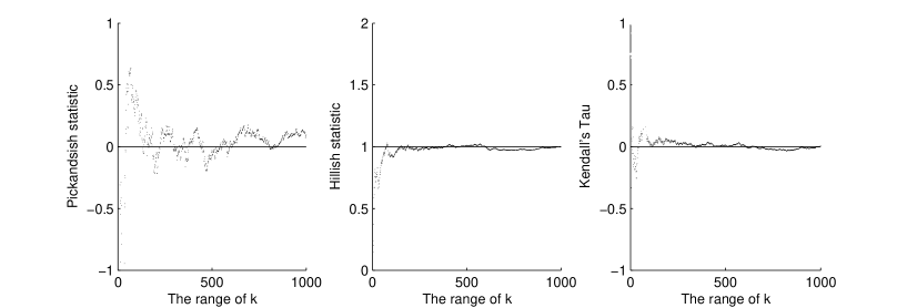
Figure 1. $\text{Pickandsish}_{k,n}(0.5)$, $\text{Hillish}_{k,n}$ and $\rho_{\tau}(k,n)$ plotted for Example 3.1

The simulated data supports the theoretical results stated.

Example 3.2.

Let $X$ and $Z$ be independent Pareto random variables where $X\sim Pareto(\rho)$ and $Z\sim Pareto(1-\rho)$ with $0<\rho<1$. Define $Y=X\wedge Z.$ Then we can check that the following holds in $\mathbb{M}_{+}([0,\infty]\times(0,\infty])$: For $x\geq y>0$ and $t$ large,

$$t\mathbf{P}\Bigl{[}\Bigl{(}\frac{X}{t},\frac{Y}{t}\Bigr{)}\in[0,x]\times(y,\infty]\Bigr{]}=\frac{1}{y^{1-\rho}}\Bigl{(}\frac{1}{y^{\rho}}-\frac{1}{x^{\rho}}\Bigr{)}=\frac{1}{y}\Bigl{(}1-\frac{y^{\rho}}{x^{\rho}}\Bigr{)}=:\mu^{*}([0,x]\times(y,\infty]).$$

Theoretically the values of the limits of $\text{Hillish}_{k,n}$ and $\text{Pickandsish}_{k,n}(p)$ are as follows.

$$\text{Hillish}_{k,n} \stackrel{{\scriptstyle\text{P}}}{{\to}}\int\limits_{1}^{\infty}\int\limits_{1}^{\infty}\mu^{*}([0,H^{\leftarrow}(\frac{1}{x})]\times(y,\infty])\frac{dx}{x}\frac{dy}{y}=\int\limits_{x=1}^{\infty}\int\limits_{y=1}^{(\frac{x}{x-1})^{1/\rho}}\frac{1}{y}\Big{(}1-\frac{y^{\rho}}{\frac{x}{x-1}}\Big{)}\frac{dx}{x}\frac{dy}{y}$$

$$=\int\limits_{x=1}^{\infty}\Big{[}1-\frac{1}{1-\rho}\frac{x-1}{x}+\frac{\rho}{1-\rho}\big{(}\frac{x-1}{x}\big{)}^{1/\rho}\Big{]}\frac{dx}{x}$$

$$=\frac{\rho}{1-\rho}\int\limits_{x=1}^{\infty}\sum\limits_{k=2}^{\infty}\binom{1/\rho}{k}\Big{(}\frac{1}{x}\Big{)}^{k+1}dx=\frac{\rho}{1-\rho}\sum\limits_{k=2}^{\infty}\binom{1/\rho}{k}\frac{1}{k}.$$

Now for $0<p<1$ we have,

$$\text{Pickandsish}_{k,n}(p) \stackrel{{\scriptstyle\text{P}}}{{\to}}\frac{H^{\leftarrow}(p)(1-2^{\rho})-\psi_{2}(2)}{H^{\leftarrow}(p)-H^{\leftarrow}(p/2)}=\frac{1-2^{\rho}}{1-\big{(}\frac{1-p}{1-p/2}\big{)}^{1/\rho}}.$$

For calculating the Kendall’s tau statistics observe that from definition we have:

$$C_{\mu^{*}}(x,y) =y\Big{(}1-\frac{1}{y^{\rho}}(1-x)\Big{)}=y-y^{1-\rho}(1-x),$$

$$dC_{\mu^{*}}(x,y) =(1-\rho)y^{-\rho}dxdy.$$

Hence we have

$$\int\limits_{0}^{1}\int\limits_{0}^{1}C_{\mu^{*}}(x,y)dC_{\mu^{*}}(x,y) =(1-\rho)\int\limits_{0}^{1}\int\limits_{0}^{1}(y-y^{1-\rho}(1-x))y^{-\rho}dxdy$$

$$=\frac{1-\rho}{2-\rho}-\frac{1}{4}.$$

Therefore

$$\rho_{\tau}(k,n) \stackrel{{\scriptstyle\text{P}}}{{\to}}4\int\limits_{0}^{1}\int\limits_{0}^{1}C_{\mu^{*}}(x,y)dC_{\mu^{*}}(x,y)-1=\frac{4(1-\rho)}{2-\rho}-2=-\frac{2\rho}{2-\rho}.$$

For $\rho=0.5$ and $p=0.5$, theoretically we have

$$\text{Hillish}_{k,n}\stackrel{{\scriptstyle\text{P}}}{{\to}}0.5,\qquad\rho_{\tau}(k,n)\stackrel{{\scriptstyle\text{P}}}{{\to}}-0.67,\qquad\text{Pickandsish}_{k,n}(p)\stackrel{{\scriptstyle\text{P}}}{{\to}}-0.75.$$

We simulate a sample of size $n=1000$ with $\rho=0.5$ and plot the three statistics for $1\leq k\leq n$. For the Pickandsish statistic we have chosen $p=0.5$.

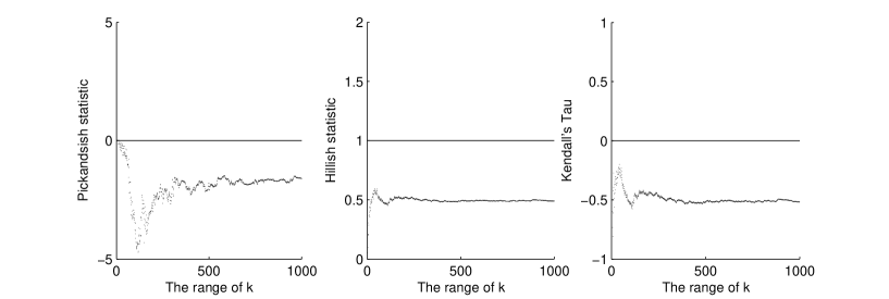
Figure 2. $\text{Pickandsish}_{k,n}(0.5)$, $\text{Hillish}_{k,n}$ and $\rho_{\tau}(k,n)$ plotted for Example 3.2

The graphs are consistent with the obtained theoretical limits.

3.2. Internet traffic data

Internet traffic data has often provided scope for heavy-tail modeling. Variables such as file size, transmission duration and session length have been observed to be heavy-tailed (Maulik et al., 2002, Resnick, 2003, Sarvotham et al., 2005).

We study a particular data set of GPS-synchronized traces that were recorded at the University of Auckland http://wand.cs.waikato.ac.nz/wits. The raw data contains measurements on packet size, arrival time, source and destination IP, port number, Internet protocol, etc. We consider traces corresponding exclusively to incoming TCP traffic sent on December 8, 1999, between 3 and 4 p.m. The packets were clustered into end-to-end (e2e) sessions which are clusters of packets with the same source and destination IP address such that the delay between arrival of two successive packets in a session is at most two seconds. We observe three variables $\{(S_{i},L_{i},R_{i}):1\leq i\leq 54353\}$:

$$S_{i} =\text{size or number of bytes transmitted in a session},$$

$$L_{i} =\text{duration or length of the session},$$

$$R_{i} =\frac{S_{i}}{L_{i}}~{}~{}\text{ or average transfer rate associated with a session.}$$

The data have been downloaded and processed into sessions by Luis Lopez Oliveros, Cornell University.

Figure 3. Pickands plot and moment estimate plot of the EV parameter for size, duration and transfer rate.

First we check whether the individual variables are heavy-tailed or not. The Pickands estimator and moment estimators are weakly consistent for the extreme value parameter $\gamma$ (de Haan and Ferreira (2006)) when the distribution of the variable under consideration is in $D(G_{\gamma})$ as in (1.1). We plot these estimators over $1\leq k\leq n$ and observe whether they stabilize over an interval. The Pickands plot indicates that the Pickands estimates of the extreme value parameter are stable for size and duration but not for the transfer rate. The moment plot on the other hand shows that the moment estimate of the extreme-value parameter stabilizes for duration but does not do that clearly for either size or transfer rate. Recall that the CEV model is applicable if either of the variables is in the domain of attraction of an extreme-value distribution. Clearly there is an indication that transfer rate might not be in an extreme value domain.

Now we turn to the three statistics we have devised in this paper first to detect whether we have a CEV model and then to check whether the limit measure is a product. First we consider the pair $(R,S)$ assuming the distribution of $S$ is in $D(G_{\gamma})$ for some $\gamma\in\mathbb{R}$. Then we consider the pair $(R,L)$ assuming the distribution of $L$ is in $D(G_{\lambda})$ for some $\lambda\in\mathbb{R}$.

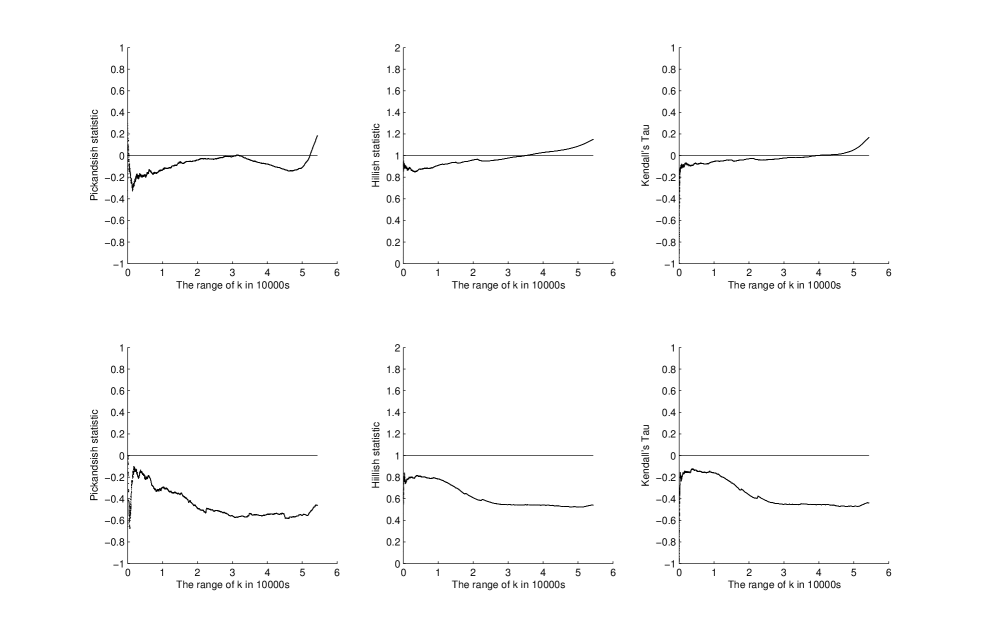
Figure 4. First row: Three statistics for $R_{i}$ vs. $S_{i}$; Second row: Three statistics for $R_{i}$ vs. $L_{i}$.

Observe from Figure 4 that neither of the three statistics stabilizes for the observations $(R,S)$. Hence a CEV model might not be the right model to apply. On the other hand for $(R,L)$, all the statistics stabilize at some point. But it is clear they are not stabilizing at a point to indicate product measure. Hence we have evidence to model (transfer rate, duration) as a CEV model with a non-product limit. Note that this also indicates that we should be able to standardize to regular variation on $[0,\infty]\times(0,\infty]$.

4. Conclusion

The CEV model is intended to provide us with a deeper understanding of multivariate distributions which have some components in an extreme-value domain. In our discussion, we have provided statistics to detect the CEV model in a bivariate set up. These three statistics perform differently for different data sets as we have noted in our examples. A further step would be to find asymptotic distributions for these statistics. On another direction, it would be nice to obtain statistics for detection of conditional models in a multivariate set up of dimension more than two.

References

• Billingsley (1968) P. Billingsley. Convergence of Probability Measures. John Wiley & Sons Inc., New York, 1968.
• Coles and Tawn (1991) S. G. Coles and J. A. Tawn. Modelling extreme multivariate events. J. R. Statist. Soc. B, 53:377–392, 1991.
• Coles et al. (1999) S.G. Coles, J.E. Heffernan, and J.A. Tawn. Dependence measures for extreme value analyses. Extremes, 2(4):339–365, 1999.
• Das and Resnick (2008a) B. Das and S. I. Resnick. QQ plots, random sets and data from a heavy tailed distribution. Stoch. Models, 24(1):103–132, 2008a. ISSN 1532-6349.
• Das and Resnick (2008b) B. Das and S. I. Resnick. Conditioning on an extreme component: Model consistency and regular variation on cones. Submitted to Bernoulli, 2008b. URL http://arxiv.org/abs/0805.4373.
• de Haan and de Ronde (1998) L. de Haan and J. de Ronde. Sea and wind: multivariate extremes at work. Extremes, 1(1):7–46, 1998.
• de Haan and Ferreira (2006) L. de Haan and A. Ferreira. Extreme Value Theory: An Introduction. Springer-Verlag, New York, 2006.
• de Haan and Resnick (1977) L. de Haan and S.I. Resnick. Limit theory for multivariate sample extremes. Z. Wahrscheinlichkeitstheorie und Verw. Gebiete, 40:317–337, 1977.
• Fougères and Soulier (2008) A. Fougères and P. Soulier. Modelling and estimation of conditional excesses. 2008. URL http://arXiv.org/0806.2426.
• Heffernan and Resnick (2007) J.E. Heffernan and S.I. Resnick. Limit laws for random vectors with an extreme component. Ann. Appl. Probab., 17(2):537–571, 2007. ISSN 1050-5164. doi: 10.1214/105051606000000835.
• Heffernan and Tawn (2004) J.E. Heffernan and J.A. Tawn. A conditional approach for multivariate extreme values (with discussion). JRSS B, 66(3):497–546, 2004.
• Hill (1975) B.M. Hill. A simple general approach to inference about the tail of a distribution. Ann. Statist., 3:1163–1174, 1975.
• Kallenberg (1983) O. Kallenberg. Random Measures. Akademie-Verlag, Berlin, third edition, 1983. ISBN 0-12-394960-2.
• Ledford and Tawn (1996) A.W. Ledford and J.A. Tawn. Statistics for near independence in multivariate extreme values. Biometrika, 83(1):169–187, 1996. ISSN 0006-3444.
• Ledford and Tawn (1997) A.W. Ledford and J.A. Tawn. Modelling dependence within joint tail regions. J. Roy. Statist. Soc. Ser. B, 59(2):475–499, 1997. ISSN 0035-9246.
• Ledford and Tawn (1998) A.W. Ledford and J.A. Tawn. Concomitant tail behaviour for extremes. Adv. in Appl. Probab., 30(1):197–215, 1998. ISSN 0001-8678.
• Mason (1982) D. Mason. Laws of large numbers for sums of extreme values. Ann. Probab., 10:754–764, 1982.
• Maulik and Resnick (2005) K. Maulik and S.I. Resnick. Characterizations and examples of hidden regular variation. Extremes, 7(1):31–67, 2005.
• Maulik et al. (2002) K. Maulik, S.I. Resnick, and H. Rootzén. Asymptotic independence and a network traffic model. J. Appl. Probab., 39(4):671–699, 2002. ISSN 0021-9002.
• McNeil et al. (2005) A.J. McNeil, R. Frey, and P. Embrechts. Quantitative Risk Management. Princeton Series in Finance. Princeton University Press, Princeton, NJ, 2005. ISBN 0-691-12255-5. Concepts, techniques and tools.
• Neveu (1977) J. Neveu. Processus ponctuels. In École d’Été de Probabilités de Saint-Flour, VI—1976, pages 249–445. Lecture Notes in Math., Vol. 598, Berlin, 1977. Springer-Verlag.
• Pickands (1975) J. Pickands. Statistical inference using extreme order statistics. Ann. Statist., 3:119–131, 1975.
• Resnick (2008) S. I. Resnick. Extreme values, regular variation and point processes. Springer Series in Operations Research and Financial Engineering. Springer, New York, 2008. ISBN 978-0-387-75952-4. Reprint of the 1987 original.
• Resnick (1999) S.I. Resnick. A Probability Path. Birkhäuser, Boston, 1999.
• Resnick (2002) S.I. Resnick. Hidden regular variation, second order regular variation and asymptotic independence. Extremes, 5(4):303–336, 2002.
• Resnick (2003) S.I. Resnick. Modeling data networks. In B. Finkenstadt and H. Rootzén, editors, SemStat: Seminaire Europeen de Statistique, Extreme Values in Finance, Telecommunications, and the Environment, pages 287–372. Chapman-Hall, London, 2003.
• Resnick (2007) S.I. Resnick. Heavy Tail Phenomena: Probabilistic and Statistical Modeling. Springer Series in Operations Research and Financial Engineering. Springer-Verlag, New York, 2007. ISBN: 0-387-24272-4.
• Resnick and Stărică (1995) S.I. Resnick and C. Stărică. Consistency of Hill’s estimator for dependent data. J. Appl. Probab., 32(1):139–167, 1995. ISSN 0021-9002.
• Sarvotham et al. (2005) S. Sarvotham, R. Riedi, and R. Baraniuk. Network and user driven on-off source model for network traffic. Computer Networks, 48:335–350, 2005. Special Issue on ”Long-range Dependent Traffic”.